ATLAS-CONF-2016-064 08/08/2016
ATLAS NOTE
ATLAS-CONF-2016-064
8th August 2016
Top-quark mass measurement in the all-hadronic t ¯ t decay channel at √
s = 8 TeV with the ATLAS detector
The ATLAS Collaboration
Abstract
The top-quark mass is measured in the all-hadronic top-antitop quark decay channel using proton–proton collisions at a centre-of-mass energy of
√s
=8 TeV with the ATLAS detector at the CERN Large Hadron Collider. The data set used in the analysis corresponds to an integrated luminosity of 20.2 fb
−1. The analysis is performed on events containing at least six jets, at least two of which must be originating from b-quarks. The reconstruction of the top quark pair and the W bosons in each event is performed using a
χ2method. The large QCD multi-jet background is modelled using a data-driven method. The top-quark mass is obtained from template fits to the ratio of the three-jet to the dijet mass. The three-jet mass is obtained from the three jets assigned to the top quark decay. From these three jets the dijet mass is obtained using the two jets assigned to the W boson decay. The top-quark mass is measured to be 173.80
±0.55 (stat.)
±1.01 (syst.) GeV.
c
2016 CERN for the benefit of the ATLAS Collaboration.
Reproduction of this article or parts of it is allowed as specified in the CC-BY-4.0 license.
1 Introduction
Of all known fundamental particles, the top quark has the largest mass. Its existence was predicted in 1973 by Kobayashi and Maskawa [1], and because of its large mass it was only first directly observed in 1995 by the CDF and D0 experiments at the Tevatron [2, 3]. Since 2010 top quarks have also been produced at the Large Hadron Collider (LHC) [4] at CERN. Due to the higher centre-of-mass energy, top quark production at the LHC is an order of magnitude larger than at the Tevatron, such that the LHC is often referred to as a “top quark factory.” The large data sets of top-antitop quark (t¯ t) pairs allow for many precision studies and measurements of top quark properties. The Yukawa coupling of the top quark is predicted to be close to unity [5, 6], suggesting that it may play a special role in electroweak symmetry breaking. The top quark dominantly contributes to the quantum corrections [7, 8] of the Higgs field, which become important for any extrapolation of the Standard Model (SM) to extremely high energies, from a few hundred GeV and above. It is at these high energies that some of the fundamental deficiencies of the SM, such as the stability of the electroweak vacuum state in the Higgs potential [9, 10], can be further investigated. Thus, precise measurements of the top-quark mass (m
top) allow for consistency tests of the SM and to look for signs of new physics beyond the SM.
Today the most precise individual measurement of m
topis in the single-lepton decay channel of top- antitop quark pairs, where one top quark decays into a b-quark, a charged lepton and a neutrino and the other top quark decays into a b-quark and two u
/d
/c
/s-quarks. This measurement was performed by the CMS Collaboration, yielding a value of m
top =172.35
±0.16 (stat.)
±0.48 (syst.) GeV [11]. The most precise measurement of m
topin the di-leptonic t¯ t decay channel, where each of the top quarks decays into a b-quark, a charged lepton and its neutrino, is from the ATLAS Collaboration, yielding a value of m
top =172.99
±0.41 (stat.)
±0.74 (syst.) GeV [12]. Further m
topresults are available in Refs [12–14].
The top-quark mass measurement in the all-hadronic t¯ t channel takes advantage of the largest branching ratio (46%) among the possible top quark decay channels [15]. The all-hadronic channel involves six jets at leading order, two originating from b-quarks and four originating from the hadronic decay of two W bosons. It is a challenging measurement because of the large multi-jet background arising from vari- ous quantum chromodynamics (QCD) processes, which can exceed the t¯ t production by several orders of magnitude. At the same time, all-hadronic t¯ t events profit from having no neutrinos in the decay products, so that all four-momenta can be directly measured. The multi-jet background for the all-hadronic t¯ t chan- nel, while large, leads to di
fferent systematic uncertainties than in the case of the single- and di-leptonic t¯ t channels. Thus, all-hadronic analyses offer an opportunity to cross check top-quark mass measurements already performed in the other channels. The most recent measurements of m
topin the all-hadronic chan- nel are performed by the CMS Collaboration with m
top =172.32
±0.25 (stat.)
±0.59 (syst.) GeV [11], and the ATLAS Collaboration with m
top=175.1
±1.4 (stat.)
±1.2 (syst.) GeV [16].
This paper presents a top-quark mass measurement in the t¯ t all-hadronic channel using data collected by the ATLAS experiment in 2012. The m
topmeasurement is obtained from template fits to the ratio (R
3/2 =m
j j j/mj j) of three-jet to dijet masses, similar to a previous measurement at
√s
=7 TeV [16]. The
three-jet mass is obtained from the three jets assigned to the top quark decay. From the selected three
jets the dijet mass is obtained using the two jets assigned to the W boson decay. The jet assignment is
accomplished by using a
χ2fit to the t¯ t system, so there are two values of R
3/2measured in each event. The
observable R
3/2employed in this analysis achieves a partial cancellation of systematic e
ffects common
to the masses of the reconstructed top quark and associated W boson, notably the significant uncertainty
due to the jet energy scale. Data-driven techniques are used to estimate the contribution from multi-jet
observables, with the signal region containing the largest relative fraction of t¯ t events. The background is derived from the other regions, determining the shape of the background distribution in the signal region.
In the following, after a brief description of the ATLAS detector in Section 2, the data and Monte Carlo (MC) samples used in the analysis are described in Section 3. The analysis event selection is further detailed in Section 4. Section 5 describes the method used to select the candidate four-momenta that comprise the reconstructed t¯ t system. The estimation of the multi-jet background is detailed in Section 6.
The method used to measure the top-quark mass and its uncertainties are reported in Sections 7, 8, and 9. The results of the measurement are presented in Section 10, and the analysis is summarised in Section 11.
2 ATLAS detector
The ATLAS detector [17] is a multi-purpose particle physics experiment with a forward-backward sym- metric cylindrical geometry and near 4π coverage in solid angle. The inner tracking detector (ID) covers the pseudorapidity
1range
|η|<2.5, and consists of a silicon pixel detector, a silicon microstrip detector, and, for
|η| <2.0, a transition radiation tracker. The ID is surrounded by a thin superconducting solen- oid providing a 2 T magnetic field. A high-granularity lead
/liquid-argon (LAr) sampling electromagnetic calorimeter covers the region
|η| <3.2. A steel
/scintillator-tile calorimeter provides hadronic coverage in the range
|η| <1.7. LAr technology is also used for the hadronic calorimeters in the endcap region 1.5
< |η| <3.2 and for both electromagnetic and hadronic measurements in the forward region up to
|η|<
4.9. The muon spectrometer surrounds the calorimeters. It consists of three large air-core supercon- ducting toroid systems, precision tracking chambers providing accurate muon tracking for
|η|<2.7, and additional detectors for triggering in the region
|η|<2.4.
3 Data and Monte Carlo simulation
This analysis is performed using the proton–proton (pp) collision data set at a centre-of-mass energy of
√s
=8 TeV. collected with the ATLAS detector at the LHC. The data correspond to an integrated luminosity of 20.2 fb
−1. Samples of simulated MC events are used to optimise the analysis, to study the detector response and the e
fficiency to reconstruct t¯ t events, to build signal template distributions used for fitting the top-quark mass, and to estimate systematic uncertainties. Most of the MC samples used in the analysis are based on a full simulation of the ATLAS detector [18] (FADS) obtained using GEANT4 [19].
Some of the systematic uncertainties are studied using alternative t¯ t samples processed through a faster ATLAS simulation (AFII) using parameterised showers in the calorimeters [20]. Additional simulated pp collisions generated with P
ythia[21] are overlaid to model the effects from additional collisions
1The coordinate system used to describe the ATLAS detector is briefly summarised here. The nominal interaction point is defined as the origin of the coordinate system, while the beam direction defines thez-axis and thex-yplane is transverse to the beam direction. The positivex-axis is defined as pointing from the interaction point to the centre of the LHC ring and the positivey-axis is defined as pointing upwards. The azimuthal angleφis measured around the beam axis, and the polar angleθis the angle from the beam axis. The pseudorapidity is defined asη=−ln tan(θ2). The transverse momentumpT, the transverse energyET, and the missing transverse momentum (EmissT ) are defined in the x-y plane unless stated otherwise. The distance∆Rin the pseudorapidity-azimuthal angle space is defined as∆R= p
∆η2+ ∆φ2.
in the same and nearby bunch crossings (pile-up). All simulated events are processed using the same reconstruction algorithms and analysis chain as used for the data.
The nominal t¯ t simulation sample is generated using the next-to-leading order (NLO) MC program POWHEG-BOX [22–24] with the NLO parton density function (PDF) set CT10 [25, 26], interfaced to P
ythia6.427 [27] with the P
erugia2012 tune [28] for parton shower, fragmentation and underlying event modelling. For the construction of the signal templates, MC samples are generated at five di
fferent as- sumed values of m
top, between 167.5 and 177.5 GeV, in steps of 2.5 GeV. The FADS sample at 172.5 GeV has the largest number of generated events, and is used as the nominal signal sample. The h
damppara- meter [29], which regulates the high-p
Tradiation in POWHEG-BOX, is set to the same m
topvalue as used in each of the generated POWHEG-BOX samples. All the simulated samples used to estimate systematic uncertainties are further described in Section 9.
All MC samples are normalised using the predicted top-antitop quark pair cross-section (σ
t¯t) at
√s
=8 TeV. For m
top =172.5 GeV, the next-to-next-to-leading-order cross section of
σtt¯ =253
+13−15pb is calculated using the program Top
++2.0 [30], which includes re-summation of next-to-next-to-leading logarithmic soft gluon terms.
4 Event selection
Events in this analysis are selected by a trigger [31, 32] that requires at least five jets with p
T >55 GeV.
Only events with a well reconstructed primary vertex formed by at least five tracks are considered for the analysis. Events with isolated electrons (muons) with E
T >25 GeV (p
T >20 GeV) and reconstructed in the central region of the detector within
|η|<2.5 are rejected. Further details on the lepton identification are given in Refs. [33, 34]. Jets ( j) are reconstructed using the anti-k
Talgorithm with radius parameter R
=0.4 [35] employing calorimeter topological clusters [36]. These jets are calibrated to the hadronic energy scale as described in Refs. [37–39]. The highest-energy muon (µ) from among those matched within
∆R( j, µ)
<0.3 to a reconstructed jet, is added to the reconstructed jet by a four-vector sum. This is done to compensate for the energy losses in the calorimeter arising from semi-leptonic quark decays.
In simulation this correction slightly improves both the jet energy response and resolution across the full range of jet energies.
To ensure that the selected events are in the plateau region of the trigger e
fficiency curve where the trigger efficiency in data is greater than 90%, at least five of the reconstructed central jets (within
|η| <2.5) are required to have p
T >60 GeV. Any additional selected jets are required to have p
T >25 GeV. All selected jets in an event need to be isolated; any pairing of two jets ( j
iand j
k) reconstructed with the above criteria are required to not overlap within
∆R( j
i,j
k)
<0.6. Events with jets failing this isolation requirement are rejected.
Events containing leptons that include neutrinos are removed by requiring E
missT <60 GeV. The E
Tmissin an event is computed as the sum of a number of different terms [40, 41]. Muons, electrons and jets are accounted for using the appropriate calibrations for each object. For each term considered, the missing transverse energy is calculated as the negative sum of the calibrated reconstructed objects, projected onto the x and y directions.
For the final selection, events are kept if at least two of the six leading transverse momentum jets are
identified as originating from a b-quark. Such jets are said to be b-tagged. A neural network trained
Event yields (thousands)
Cut Data t¯ t all-hadronic (MC)
Initial 850450 2338
±1
Primary vertex with
>4 tracks - -
No high-p
Tisolated e
/µ- -
Jets
|η|<2.5 33476 308.7
±0.6
Trigger: 5 jets with p
T>55 GeV 16110 241.4
±0.5 No 2 good jets ( j
i,j
k) in
∆R( j
i,j
k)
<0.6 7646 142.9
±0.4
≥
6 jets with p
T >25 GeV 7646 142.9
±0.4
≥
5 jets with p
T >60 GeV 3303 51.4
±0.2
E
missT <60 GeV 3021 46.3
±0.2
∆φ(bi,
b
j)
>1.5 1737 30.9
±0.2
χ2<
11 645.8 22.3
±0.1
N
btag ≥2 21.9 6.61
±0.08
h∆φ(b,
W)i
<2 12.9 4.40
±0.07
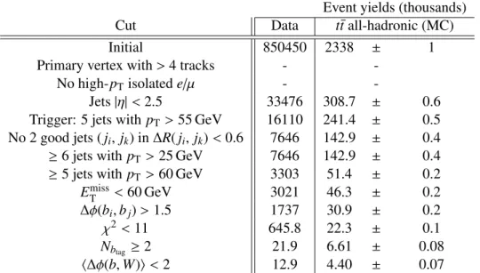
Table 1: A summary of the event yields following each of the individual event selection cuts, with values shown for both data and all-hadronic MC events generated atmtop =172.5 GeV (shown with statistical uncertainty). The tt¯contribution is after scaling to the theoretical cross-section and integrated luminosity. The cuts in the second and third row refer to pre-selection requirements. Their inclusive yields are listed as “Initial” in the first row.
c-quarks coming from the W boson decay in this analysis (on average one c-quark per event) a b-tagger trained to reject u
/d
/s-jets but also a larger fraction of c-jets is used. Events with fewer than two b-tagged jets are used for the background estimate described in Section 6. The b-tagging neural network provides an identification e
fficiency of about 57% [43] for jets from b-quarks, with a rejection factor of about 180 for jets arising from u
/d
/s-quarks, and a factor of about seven for jets arising from c-quarks.
In each event the two leading b-tagged jets (b
iand b
j) are required to satisfy the requirement
∆φ(bi,b
j)
>1.5. Leading here means that b-tagged jets are ordered according to their assigned b-tag weight. The indices i and j stand for the position of the leading b-tagged jets within the p
Tordered list of good reconstructed jets. This
∆φcut is very powerful at rejecting combinatorial background events; most of these are true t¯ t events where the incorrect jets are associated to the top quark. Finally, a cut is applied based on the separation in azimuthal angle between b-tagged jets and their associated W boson candidate:
the average of the two angular separations for each event is required to satisfy
h∆φ(b,W)i
<2. The W boson candidates are identified by means of the jets combination which fits best the t¯ t event hypothesis described in Section 5. This
∆φcut rejects a large fraction of events from the multi-jet and combinatorial backgrounds, as well as events from non-all-hadronic t¯ t decays. Events failing this final selection cut are however retained for the purpose of modelling the multi-jet background, as detailed in Section 6.
Table 1 summarises the yields obtained after each of the individual selection cuts. The
χ2cut listed
in Table 1 is described in Section 5. The number of b-tagged jets (N
btag) and
h∆φ(b,W)i are the two
observables used for the data-driven multi-jet background estimation, further detailed in Section 6.
5 t ¯ t reconstruction
In each event the t¯ t final state is reconstructed using all the jets from the all-hadronic t¯ t decay chain:
t¯ t
→bWbW
→b
1j
1j
2b
2j
3j
4. To determine the top-quark mass in each t¯ t event, a minimum
χ2approach is adopted, with the
χ2defined as:
χ2=
(m
b1j1j2−m
b2j3j4)
2 σ2∆mb j j
+
(m
j1j2−m
MCW)
2 σ2mMC
W
+
(m
j3j4−m
MCW)
2 σ2mMC
W
.
(1)
Here, two of the reconstructed jets are associated with the bottom-type quarks produced directly from the top quark and anti-top quark decays (b
1and b
2), the other four jets are assumed to be u
/d
/c
/s-quark jets coming from the W boson hadronic decay ( j
i, where i
=1, . . . , 4), and
∆m
b j j =m
b1j1j2 −m
b2j3j4. This method considers all possible permutations of the six or more reconstructed jets in each event.
The permutation resulting in the lowest
χ2value is kept. A low
χ2value denotes a permutation of jets consistent with the t¯ t hypothesis. No explicit b-tagging information is used in in Eq. (1).
In each combination the reconstructed masses of the two hadronically decaying W bosons (m
j1j2and m
j3j4) in data are compared to the mean of the correctly reconstructed W boson mass distributions (m
MCW) in simulated signal MC events. The correct reconstruction of the top quarks and the W bosons in a simulated event is achieved by matching parton-level particles to its own jets. The width values (σ
mMCand
σ∆mb j j) used in the denominators of Eq. (1) are obtained from single Gaussian fits to these correctly
Wreconstructed mass distributions;
σ∆mb j j =21.60
±0.16 (stat.) GeV and
σmMCW =
7.89
±0.05 (stat.) GeV.
The m
MCWmean value used in Eq. (1) is determined to be 81.18
±0.04 (stat.) GeV. To reduce the multi-jet background in the analysis, a minimum
χ2<11 is required.
6 Multi-jet background estimation
The available MC generators for multi-jet production include only leading-order theory calculations for final states with up to six partons. Therefore, the dominant multi-jet background in this analysis is de- termined directly from the data. Two largely uncorrelated variables are used to divide the data events into four different phase space regions, such that the background is derived from the control regions and ex- trapolated into the signal region. The two chosen observables are the N
btagin an event, and the
h∆φ(b,W)i quantity, both described in Section 4. These have a correlation measured in data of
ρ=−0.038. The value of N
btagin each event is determined from the leading six jets only.
The four regions, labelled ABCD, are identified by defining two bins in the number of b-tagged jets,
N
btag <2, N
btag ≥2, and two ranges of the
h∆φ(b,W)i quantity,
h∆φ(b,W)i
<2.0,
h∆φ(b,W)i ≥ 2.0, as
detailed in Table 2. The R
3/2distributions are studied for each of the defined regions. Region D represents
the signal region (SR), and contains the largest fraction of t¯ t events (34.05%). Regions A, B, and C are the
control regions (CR), and are dominated by multi-jet background events. The summary of the expected
fractions of signal events in each of the four regions is given in Table 2. Each signal fraction is estimated
by comparing the total predicted number of signal events from t¯ t simulation to the number of observed
data events in each region.
ABCD Region and Definition Estimated Signal Fraction Region N
btag h∆φ(b,W)
it¯ t MC/data [%]
A
<2 ≥2.0 2.06
±0.02
B
<2 <2.0 2.60
±0.02
C
≥2 ≥2.0 24.71
±0.55
D
≥2 <2.0 34.05
±0.57
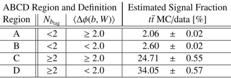
Table 2: Definitions and signal fractions for each of the four regions used to estimate the multi-jet background.
Region D is the signal region. The signal fraction is estimated by comparing the total predicted number of signal events fromtt¯simulation to the number of observed data events in each region.
To obtain an unbiased estimate of the number of background events in each considered CR, the signal con- tamination needs to be removed. The estimated background in a given bin i of R
3/2for SR D (N
background,iSR D) is given by:
N
background,iSR D =
N
backgroundCR CN
backgroundCR A
N
background,iCR B .(2)
The right-hand side of the above equation represents the bin i of the R
3/2spectrum of CR B after sub- traction of the signal contamination and after scaling by the ratio of the number events in control regions C (N
backgroundCR C) and A (N
CR Abackground) also after signal removal. The analysis is not sensitive to the signal contamination present in CR C, as this region only affects the normalisation of the distribution obtained for the multi-jet background, which is not used in the fit for m
topdescribed in Section 7.
Figure 1 shows the distributions of the masses of the W boson (m
j j) and top quark (m
j j j) after applying the event selection, the
χ2approach defined in Eq. (1), and using the data-driven multi-jet background method. In the figure, the reconstruction using MC events is said to be correct for one (or both) top quark(s) if each of the three jets ( j) selected by the reconstruction algorithm matches to each of the three quarks (q) within a
∆R( j, q)
<0.3, modulo the interchange of the two jets assigned to the hadronically decaying W boson. If at least one of the jets selected by the algorithm is not one of the three jets matched to the quarks, the top quark reconstruction is classified as incorrect. Finally, events where at least one quark is not matched uniquely to a reconstructed jet are classified as non-matched. The R
3/2distribution obtained after using the data-driven multi-jet background methods to determine the shape and normalisa- tion is shown in Figure 2. In general, good agreement between data and prediction is observed in all the distributions.
7 Top-quark mass determination
To extract a measurement of the top-quark mass, a template method with a binned minimum
χ2approach is employed. The value of R
3/2is calculated on an event-by-event basis, and for each event two R
3/2values are obtained. To properly correct for the correlation between the two R
3/2values, the statistical uncertainty on m
topreturned from the final
χ2fit described later in this section is scaled up by a factor
p1
+ρ≈1.26,
where
ρ =0.59 is the correlation factor as obtained from data. Signal and background binned templates
Entries / 2 GeV
500 1000 1500 2000 2500 3000
ATLASPreliminary Ldt = 20.2 fb-1
∫
= 8 TeV s Data
MC (Correct) t t
MC (Incorrect) t t
MC (Non-Matched) t
t
QCD Multi-jet (Data-Driven) Syst. Uncertainty Stat.⊕
[GeV]
mjj
60 70 80 90 100 110 120 130
Data / Prediction
0.5 1 1.5
Entries / 3 GeV
200 400 600 800
1000 ATLASPreliminary Ldt = 20.2 fb-1
∫
= 8 TeV s Data
MC (Correct) t t
MC (Incorrect) t t
MC (Non-Matched) t
t
QCD Multi-jet (Data-Driven) Syst. Uncertainty Stat.⊕
[GeV]
mjjj
140 160 180 200 220 240 260 280 300
Data / Prediction
0.5 1 1.5
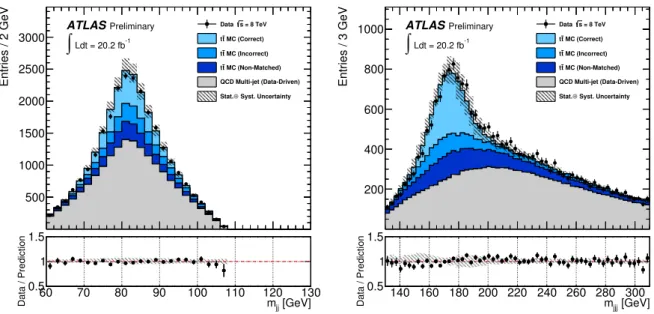
Figure 1: Dijet invariant mass distribution,mj j, forWboson candidates (left) and three-jet invariant mass,mj j j, for top quark candidates (right) in data compared to the sum oft¯tMC and multi-jet background. The ratio compar- ing data to prediction is shown below each distribution. The hatched bands reflect the sum of the statistical and systematic errors added in quadrature. Thett¯MC corresponds tomtop=172.5 GeV.
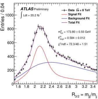
Entries / 0.04
200 400 600 800 1000
ATLASPreliminary Ldt = 20.2 fb-1
∫
= 8 TeV s Data
MC (Correct) t t
MC (Incorrect) t t
MC (Non-Matched) t
t
QCD Multi-jet (Data-Driven) Syst. Uncertainty
⊕ Stat.
/mjj
= mjjj
R3/2
1.6 1.8 2 2.2 2.4 2.6 2.8 3 3.2 3.4
Data / Prediction
0.5 1 1.5
Figure 2:R3/2 distribution in data shown together with the expected sum oft¯tMC and multi-jet background. The ratio comparing data to prediction is shown below the figure. The hatched bands reflect the sum of the statistical and systematic errors added in quadrature. Thett¯MC corresponds tomtop=172.5 GeV.
in R
3/2are created using the simulated t¯ t events described in Section 3, and the data-driven background distribution.
The top quark contribution is parameterised by a probability distribution function (p.d.f.) which is the sum of a Novosibirsk
2and Landau [44] functions. These describe, respectively, the signal and the combinatorial background. This parameterisation involves six parameters describing the shape of the R
3/2distribution. As a first step, the R
3/2distributions from the five t¯ t simulation samples with di
ffering m
topare fitted separately to determine the six parameters for each template mass. The MC simulation shows that each of these parameters depends linearly on the input m
top. In the next step, the parameters are fitted to obtain the o
ffsets and slopes of the linear m
topdependencies. These values are then used as inputs to a combined, simultaneous fit to all five R
3/2distributions. In total 12 parameters are derived by the combined fit to determine the p.d.f. Figure 3 shows the R
3/2distributions obtained using the FADS t¯ t MC samples generated at three top-quark mass points: 167.5, 172.5, and 175 GeV. Results from the combined, simultaneous fit to all five R
3/2distributions are superimposed. Shown are the functions describing the signal and combinatorial background, respectively, and their sum. The Novosibirsk mean and width parameters o
ffer the strongest sensitivity to m
top. The overall sensitivity of the R
3/2shape to m
topis seen in Figure 4.
The background template distribution obtained from the output of the data-driven method described in Section 6 can be parameterised in a similar fashion. In this case the sum of a Gaussian and Landau function was found to be a suitable choice for the functional form. The background p.d.f. requires five parameters.
As a final step in the parameterisation, in order to take properly into account the uncertainties and the correlations between the various signal and background shape parameters, a more generalised version of the
χ2function is used. The final
χ2fit which uses matrix algebra, important to include non-diagonal covariance matrices, has the form:
χ2 =
Nbin
X
i=1 Nbin
X
k=1
(n
i−µi) (n
k−µk)
hV
data+V
signal(m
top,F
bkgd)
+V
bkgd(F
bkgd)
i−1ik.
(3)
Here m
topand F
bkgdare the two parameters which are left to float. The shape of the fitted parameterisa- tion is assumed to be independent of m
topwhile the normalisation, controlled by a background fraction parameter, F
bkgd, is obtained by fitting the data distribution. The F
bkgdis defined within the fit range of the R
3/2distribution: 1.5
≤R
3/2 <3.5. The term n
icorresponds to the number of entries in the R
3/2data distribution, whereas
µicorresponds to the number of estimated signal and background combined entries. V
datais the N
bin ×N
bindata covariance matrix which takes into account the uncertainties with relative correlation in the numbers of measured data entries in each given bin. Similarly V
signaland V
bkgdare N
bin×N
binnon-diagonal covariance matrices, which account for the signal and background shape parameterisation.
2The Novosibirsk function is defined by: f(mES) = ASexp(−0.5ln2[1+ Λτ·(mES−m0)]/τ2+τ2), where AS is a constant, mESis the measured mass,Λ =sinh(τ√
ln 4)/(στ√
ln 4), the peak position ism0, the width isσ, andτis the tail parameter.
/mjj
= mjjj
R3/2
Entries / 0.04
500 1000 1500 2000
2500 tt MC s = 8 TeV
Novosibirsk Landau Total Fit (Global)
ATLAS
Preliminary Preliminary
Simulation
q q b q bq b→ bW- W+ t→ t
= 167.5 GeV gen
mtop
/mjj
= mjjj
R3/2
1.6 1.8 2 2.2 2.4 2.6 2.8 3 3.2 3.4
σFit/
2
− 0 2
/mjj
= mjjj
R3/2
Entries / 0.04
2000 4000 6000 8000
10000 tt MC s = 8 TeV
Novosibirsk Landau Total Fit (Global)
ATLAS
Preliminary Preliminary
Simulation
q q b q bq b→ bW- W+ t→ t
= 172.5 GeV gen
mtop
/mjj
= mjjj
R3/2
1.6 1.8 2 2.2 2.4 2.6 2.8 3 3.2 3.4
σFit/
2
− 0 2
/mjj
= mjjj
R3/2
Entries / 0.04
500 1000 1500 2000 2500
3000 tt MC s = 8 TeV
Novosibirsk Landau Total Fit (Global)
ATLAS
Preliminary Preliminary
Simulation
q q b q bq b→ bW- W+ t→ t
= 175.0 GeV gen
mtop
/mjj
= mjjj
R3/2
1.6 1.8 2 2.2 2.4 2.6 2.8 3 3.2 3.4
σFit/
2
− 0 2
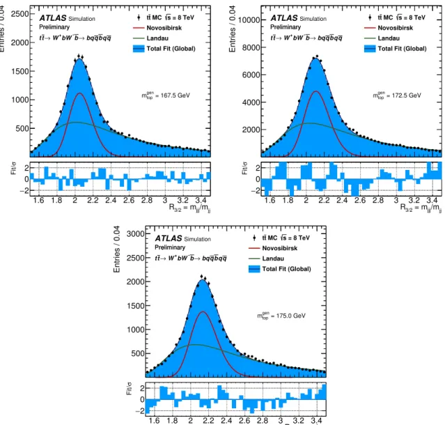
Figure 3: Templates for theR3/2 distributions for t¯t MC samples generated at mtop values of 167.5, 172.5, and 175 GeV, respectively. Results from the combined, simultaneous fit to all fiveR3/2distributions are superimposed (black line with blue, filled area). For each distribution it consists of a Novosibirsk function (red line) describing the signal part and a Landau function (green line) describing the combinatorial background part. Their parameters are assumed to depend linearly onmtop. Theχ2 over the number of degrees of freedom obtained for each of the three template distribution corresponds to 1.22, 3.98, and 2.02 respectively. The insets under each distribution show the residuals obtained from calculating the difference between the combined fit and the simulatedR3/2distribution normalised to the statistical uncertainty for each bin individually.
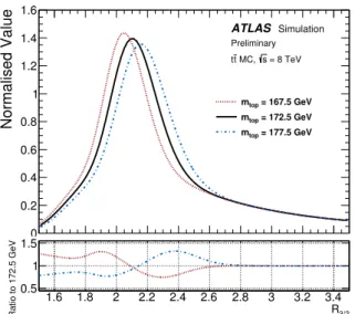
Normalised Value
0 0.2 0.4 0.6 0.8 1 1.2 1.4 1.6
ATLAS Preliminary
Simulation = 8 TeV s MC, t t
= 167.5 GeV mtop
= 172.5 GeV mtop
= 177.5 GeV mtop
R3/2
1.6 1.8 2 2.2 2.4 2.6 2.8 3 3.2 3.4
Ratio to 172.5 GeV
0.5 1 1.5
Figure 4: Template distributions shown simultaneously for three separate input values ofmtop (167.5, 172.5, and 177.5 GeV), highlighting the sensitivity of theR3/2shape tomtop. The inset under the distribution shows the ratio of mtopat 167.5, and 177.5 GeV tomtopat 172.5 GeV.
8 Method validation and template closure
To validate the method employed to extract m
topfrom the R
3/2data distribution and to check for any potential bias, a series of pseudo experiments are performed. For each of the five simulated m
topsamples a total of 2500 pseudo experiments of the R
3/2variable are produced
3. Two scenarios are investigated: in the first one, events are drawn randomly from template R
3/2distributions; in the second scenario, events are drawn directly from the signal and background shapes. In all cases the nominal values of all signal and background shape parameters are used, and only two parameters, m
topand F
bkgd, are left to be returned from the minimisation procedure. For all five top-quark mass MC samples, the same multi-jet background distribution is used for drawing pseudo events.
The value of m
topobtained from each pseudo experiment (m
meastop) is used to fill a distribution of the difference between these values and the generated values for m
top, m
gentop. This distribution is then fitted with a Gaussian function, giving estimators for the Gaussian mean and width parameters, each with their respective uncertainties. The uncertainty on the fitted mean is corrected for the oversampling that is induced by drawing from template distributions produced using a finite number of MC events [45].
The fitted mean
Dm
meastop −m
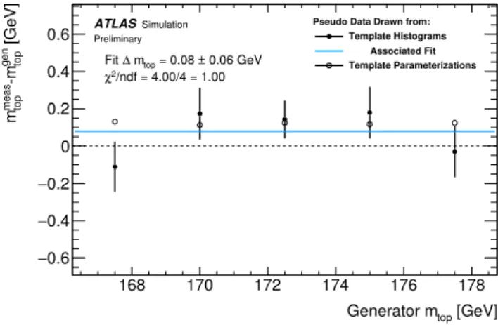
gentopE, referred to as the “difference mean”, is shown in Figure 5. Fitting the difference mean for the five top mass samples with a zero-order polynomial results gives an m
gentop- independent bias of 0.08±0.06 GeV. The treatment of this small bias is further discussed in Section 9.2.
Pull distributions are constructed in an analogous way, where the pull in each pseudo experiment is defined as:
Pull
=m
meastop −m
gentop/δmtop
(4)
3This value of 2500 is also used when performing pseudo experiments to evaluate the systematic uncertainties.
where
δmtopis the statistical uncertainty on the m
topparameter obtained from the fit of the pseudo exper- iment. Note that the correction for taking into account the correlation between two R
3/2values in each event, described in Section 7, is not applied here, as the values of R
3/2drawn for pseudo experiments are drawn without taking into account any correlation. The pull distribution for an unbiased measurement has a mean of zero and a standard deviation of unity. A fitted pull mean value of 0.19
±0.13 and a fitted pull width of 0.98
±0.01 are obtained, which shows that the uncertainty determination is unbiased.
[GeV]
Generator mtop
168 170 172 174 176 178
[GeV]gen top-mmeas topm
0.6
− 0.4
− 0.2
− 0 0.2 0.4 0.6
0.06 GeV = 0.08 ± mtop
Fit ∆
Pseudo Data Drawn from:
Template Histograms Associated Fit Template Parameterizations /ndf = 4.00/4 = 1.00
χ2
ATLAS Preliminary
Simulation
Figure 5: The difference mean,
mmeastop −mgentop
, based on the results of a single Gaussian fit. The black markers correspond to cases where the pseudo events were drawn from theR3/2 histograms, and the open marker points where pseudo events were drawn from the parameterisations. The solid blue line corresponds to a polynomial fit to the five black markers and their corrected uncertainties.
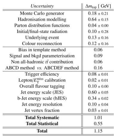
9 Systematic uncertainties
This section outlines the various sources of systematic uncertainty on m
topwhich are summarised in Table 3. All sources are treated as uncorrelated. Individual contributions are symmetrised and the total uncertainty is taken as the quadratic sum of all contributions.
The majority of the systematic uncertainties are assessed by varying the source of uncertainty in the t¯ t MC sample. Pseudo experiments are constructed from the varied sample, which are then passed through the analysis chain; the di
fference in the result when compared to that obtained from the nominal MC sample is evaluated. Exceptions to this are described in the following sub-sections.
In what follows, each of the systematic sources are briefly described. These are broken down into three
categories. The first category, theory and modelling-related uncertainties, is associated with the simu-
lation of the signal events. The second, method-related uncertainties, involve uncertainties in the way
that the analysis has been performed, including the choice of a template method, the background mod-
elling, and the final m
topextraction procedure. Finally a third category, calibration- and detector-related
uncertainties involves uncertainties coming from the standard calibrations of physics objects.
Uncertainty
∆m
top[ GeV]
Monte Carlo generator 0.18
±0.21Hadronisation modelling 0.64
±0.15Parton distribution functions 0.04
±0.00Initial/final-state radiation 0.10
±0.28Underlying event 0.13
±0.16Colour reconnection 0.12
±0.16Bias in template method 0.06 Signal and bkgd parameterisation 0.09 Non all-hadronic t¯ t contribution 0.06 ABCD method vs. ABCDEF method 0.16
Trigger e
fficiency 0.08
±0.01Lepton/ E
missTcalibration 0.02
±0.01Overall flavour tagging 0.10
±0.00Jet energy scale (JES) 0.60
±0.05b-Jet energy scale (bJES) 0.34
±0.02Jet energy resolution 0.10
±0.04Jet vertex fraction 0.03
±0.01Total Systematic 1.01
Total Statistical 0.55
Total 1.15
Table 3: Summary of all sources of statistical and systematic uncertainties on the measured values of the top- quark mass. Totals are evaluated by means of a quadratic sum and under the assumption that all contributions are uncorrelated. The uncertainties are subdivided into three categories: theoretical uncertainties, method-related uncertainties, and calibration- or detector-related uncertainties, as described in the text. Adjacent to each of the quoted systematic variations onmtopis its associated statistical uncertainty, listed in a smaller font. The ABCDEF method is further described in Section9.2and in Ref. [16]. The quoted statistical uncertainty is corrected for the R3/2correlation between the two measurements of each event.
9.1 Theory- and modelling-related uncertainties
Monte Carlo generator: In order to assess the impact on the m
topmeasurement due to the choice of MC generator, the results of pseudo experiments using two di
fferent AFII simulated samples are com- pared: one sample produced using POWHEG-BOX as the MC generator and a second sample using MC@NLO [46]. Both samples use H
erwig6.520.2 [47] with the AUET2 tune to model the parton shower, hadronisation and underlying event, in contrast with the nominal signal MC where P
ythia6.427 is used.
The absolute difference of 0.18 GeV in the resulting average m
topparameter returned from the fits is quoted as the uncertainty.
Hadronisation modelling: To quantify the expected di
fference in the measured m
topvalue due a choice
of hadronisation model, pseudo experiments are performed for two independent MC samples both em-
ploying POWHEG-BOX AFII simulation to generate the all-hadronic t¯ t events but di
ffering in their choice
of hadronisation model. In the first case P
ythia6.427 [27] is used to provide the parton shower, hadron-
isation and underlying event models with the Perugia 2012 tunes [28], while in the second case, Herwig
6.520.2 with the AUET2 tune [47] is used. The absolute di
fference of 0.64 GeV between the average m
topvalue obtained in the two cases is quoted as the systematic uncertainty.
Parton distribution functions: A variety of PDF sets is investigated in order to assess the impact of the choice of CTEQ10 [25, 26], the default PDF set used in the nominal measurement. There are a total of 53 distinct sets for the CTEQ PDFs. In addition there are 101 distinct NNPDF23 [48] PDF sets and 41 distinct MSTW2008 [49, 50] PDF sets to consider for a total of 195 distinct sets to compare. Simulated POWHEG
+H
erwig[22–24, 47] events are used for the comparison, and for each di
fferent PDF set used, pseudo experiments are built by reweighting to the corresponding PDF sets. Pseudo experiments are then performed with the modified normalisation taken into account, and the resulting average m
topvalues obtained in each of the 195 cases are compared. For the CTEQ10 PDFs, the di
fference between the up and down variations are added in quadrature, and half the quadratic sum is taken as total deviation for the CTEQ10 PDF sets. A similar procedure is adopted for the MSTW and NNPDF sets. The final quoted value corresponding to 0.04 GeV is evaluated by selecting the largest deviation from the m
topnominal value for each type of PDF set with respect to either the up or down variation.
Initial-state and final-state radiation: Varying the amount of initial- and final-state radiation (ISR and FSR) can have an impact on the number of reconstructed jets, which in turn can a
ffect the overall meas- urement of the top-quark mass. In order to quantify the sensitivity of the measurement to ISR/FSR, two alternative POWHEG-BOX plus P
ythia6.427 [27] AFII samples are used. The first sample has the h
dampparameter [29] set to 2m
top, the factorisation and renormalisation scale decreased by a factor of 0.5 and uses the Perugia 2012
radHitune [28], giving more parton shower radiation. The second sample has the P
erugia2012
radL
otune, h
damp =m
topand the factorisation and renormalisation scale increased by a factor of 2, giving less parton shower radiation. Half of the absolute di
fference between the measured m
topvalues from the pseudo experiments is quoted as the corresponding systematic uncertainty, which results in a value of 0.10 GeV.
Underlying event: Additional semi-hard multiple parton interactions (MPI) present in the hard-scattering can lead to differences in the resulting kinematics of the underlying event. The amount of such additional semi-hard MPI is a P
erugia2012 tunable parameter [28] in the P
ythia6.427 generator [27]. Simulated t¯ t AFII events were produced with an increased amount of semi-hard MPI (P
erugia2012
mpiH
i) in order to assess the potential impact on the final measurement. The absolute difference between the results of these pseudo experiments and the one using the nominal simulated AFII sample is quoted as the systematic uncertainty, corresponding to a value of 0.13 GeV.
Colour reconnection: Simulated AFII signal events using P
ythia6.427 [27] for the parton shower and hadronisation modelling have a tunable parameter associated with the colour reconnection strength due to the colour flow along parton lines in the strong-interaction hard-scattering process. An alternative AFII t¯ t sample uses P
ythiaP
erugia2012
loCR tune [28], which corresponds to reduced colour recon- nection strength. The absolute di
fference of 0.12 GeV between the results of these pseudo experiments and the average m
topvalue obtained using the nominal P
ythia6.427 t¯ t events is quoted as the systematic uncertainty.
9.2 Method-dependent uncertainties
Bias in template method: Based on the results of the closure tests, a small bias is observed in the extrac-
ted top quark mass. By drawing pseudo events from the parameterisations an offset of about 100 MeV in
the mass difference (m
meas−m
gen) is present (see Figure 5). The offset does not exhibit a dependence on
pseudo experiments across m
gentopis subtracted from the final m
topvalue as measured in data. The final value of m
topquoted in this analysis includes this subtraction. The uncertainty on this fitted offset is then quoted as the systematic uncertainty of 0.06 GeV associated with the template method non-closure.
Signal and background parameterisation:
To extract m
topas described in Section 7, the uncertainties on the shape parameters of the R
3/2observable for the signal contributions are included in the N
bin×N
bincovariance matrices which enter into the
χ2minimisation used to extract m
top(see Eq. (3)). Omitting these contributions would yield a simplified definition of the
χ2variable:
χ2=
Nbin
X
bini Nbin
X
bink
(n
i−µi) (n
k−µk) [V
data]
−1ik =Nbin
X
bini
(n
i−µi)
2n
i(5)
which can be recognised as the standard definition of the
χ2variable for a least-squares fit assuming only a diagonal covariance matrix. The fit to the data distribution is repeated using this simplified definition of the
χ2variable. This results in a slightly modified value of the m
topparameter returned and a smaller statistical uncertainty. The quadratic di
fference corresponding to 0.09 GeV between the final statistical uncertainty returned from the original minimisation and this modified value is quoted as the uncertainty in the signal parameterisation.
Inclusion of non-all-hadronic
tt¯ background: A number of event selection requirements, such as the lepton veto and the requirement that E
missT <60 GeV, results in a large suppression of background con- tributions arising from non-all-hadronic t¯ t events. The estimated fractional contribution from such events in the final signal region is below 3%, and is not considered in the nominal case. Pseudo experiments are performed by drawing events from the nominal signal distribution but from a modified background, now consisting of both QCD and t¯ t events with at least one leptonic W boson decay. The absolute difference of 0.06 GeV between the average m
topvalue obtained in this way and that from the nominal case is quoted as a systematic uncertainty.
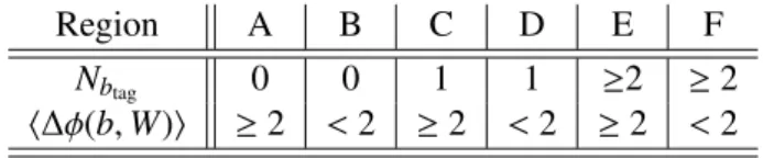
Variation in the number of control regions: A variation of the background estimation procedure is considered in which six distinct regions, rather than four, are defined to estimate the multi-jet background.
This is done by allowing for three different values of N
btag: 0, 1, or
≥2. Events can then be separated into the six di
ffering regions of phase space as in the nominal analysis. As in the nominal case the number of b- tagged jets in an event considers only the leading six jets, ordered in p
T. The values of the second ABCD variable,
h∆φ(b,W)i, are unchanged from the nominal case. One reason for considering this alternative is that the inclusion of a larger number of control regions could potentially provide sensitivity to di
fferent physics processes. Additionally, the systematic uncertainty contribution arising from uncertainties in the b-tagging scale factors could differ between these methods.
With a total of six regions shown in Table 4 the background estimation technique remains similar to that using four regions.
The final SR is labelled F. The new region D now, together with region B, is used to predict the shape of the multi-jet background in SR F, CR whereas A, C, and E set the multi-jet background normalisation [16].
Pseudo experiments are performed by drawing background events from the modified multi-jet distribution
in the final signal region. The absolute difference of 0.16 GeV between this and the nominal case is quoted
as the systematic uncertainty.
Region A B C D E F
N
btag0 0 1 1
≥2 ≥2
h∆φ(b,
W)i
≥2
<2
≥2
<2
≥2
<2
Table 4: Definitions for each of the six regions ABCDEF used to estimate the multi-jet background.
9.3 Calibration- and detector-related uncertainties
Trigger e
fficiency: The trigger e
fficiency obtained using simulated signal events [22–24, 27, 28] is com- pared to an equivalent distribution obtained using data, which results in a small discrepancy being ob- served. The data here are expected to consist primarily of multi-jet events. It is expected that some true kinematic di
fferences give rise to the di
fference observed between the data and MC trigger e
fficiencies.
In order to obtain a conservative uncertainty, it is assumed that the di
fference represents a mis-modelling of the data by the trigger simulation. The simulated events are assigned a p
T-dependent trigger efficiency correction such that the corrected MC and data trigger e
fficiencies agree. Pseudo experiments are per- formed by drawing signal events from the modified R
3/2distribution with the trigger SFs applied, and the absolute difference compared to the nominal case is quoted as a conservative uncertainty due to the trigger e
fficiency, corresponding to a value of 0.08 GeV.
Pile-up reweighting scale: The distribution of the average number of interactions per bunch crossing, de- noted by
hµi, is known to differ between data and simulation. Simulated events are reweighted so thathµimatches the value observed in data. In order to assess the impact on the final result, pseudo experiments are performed in which the reweighting scale is shifted up and down according to its uncertainty, and the fit procedure is repeated. A negligible maximum deviation of 0.01 GeV is found as the symmetrised up
/down uncertainty.
Lepton and
EmissT
soft term calibrations: Uncertainties in the calibration scales and in the resolutions of the lepton (e/µ) four-vector objects [34, 51, 52] can potentially lead to small differences in the event selection or the jet-quark assignment in the top reconstruction algorithm. Similarly, small uncertainties can be expected due to the uncertainties in the scale and resolution of the E
missTsoft term [40, 41]. The E
Tmisssoft term is varied according to these uncertainties and pseudo experiments are performed with the modified MC events. In the case of the muon-related uncertainties, Gaussian smearing is performed to assess the impact on the final result. The maximum absolute deviation from the reference m
topvalue is taken as the uncertainty in each case, and these are added in quadrature to quote a single value for all lepton and E
Tmiss-related scale and resolution uncertainties, corresponding to 0.02 GeV.
Flavour tagging e
fficiencies: In the validation of the flavour tagging algorithms, the differences between tagging e
fficiencies and mis-tag rates evaluated between data and simulation are corrected by applying scale factor (SF) weights to the simulated events. The uncertainties on the flavour tagging SFs are cal- culated separately for the b-tagging SFs, the c/τ-tagging SFs, and the overall mis-tag SFs [43]. The uncertainties on the flavour tagging SFs are split into various components. The full covariance matrix between the various bins of jet transverse momentum is built and decomposed into eigenvectors. Each eigenvector corresponds to an independent source of uncertainty, each with an upward and a downward fluctuation, with a final total quoted systematic uncertainty of 0.10 GeV.
Jet energy scale: The di
fferent contributions to the total JES uncertainty are evaluated individually as
corresponding to one-sigma deviations relative to the nominal JES, are quoted separately. The total uncertainty for each contribution is taken as half of the absolute difference between the up and down variation. In the case that both the up and down variations result in a change in the parameter in the same direction, the largest absolute di
fference (either from the up or down variation) is taken as the symmetrised uncertainty. The total JES uncertainty is the quadratic sum of all sub-contributions, corresponding to a value of 0.60 GeV. This includes all but the b-jet energy scale contribution which is quoted separately and discussed below.
b-jet energy scale:
![Table 5: Breakdown of the standard components for the jet energy scale (JES) uncertainties [34] on the measured values of the m top at √](https://thumb-eu.123doks.com/thumbv2/1library_info/4007812.1540990/22.892.300.609.217.758/table-breakdown-standard-components-energy-uncertainties-measured-values.webp)
