NLO QCD corrections to the production of Higgs plus two jets at the LHC

arXiv:1301.0493v2 [hep-ph] 26 May 2013

NLO QCD corrections to the production of Higgs plus two jets at the LHC ^✩

H. van Deurzen

^a

, N. Greiner

^a

, G. Luisoni

^a

, P. Mastrolia

^a,b

, E. Mirabella

^a

, G. Ossola

^c,d

, T. Peraro

^a

, J. F. von Soden-Fraunhofen

^a

, F. Tramontano

^e,f

a

Max-Planck-Institut f¨ ur Physik, F¨ ohringer Ring 6, 80805 M¨ unchen, Germany

b

Dipartimento di Fisica e Astronomia, Universit` a di Padova, and INFN Sezione di Padova, via Marzolo 8, 35131 Padova, Italy

c

New York City College of Technology, City University of New York, 300 Jay Street, Brooklyn NY 11201, USA

d

The Graduate School and University Center, City University of New York, 365 Fifth Avenue, New York, NY 10016, USA

e

Dipartimento di Scienze Fisiche, Universit` a degli studi di Napoli “Federico II”, I-80125 Napoli, Italy

f

INFN, Sezione di Napoli, I-80125 Napoli, Italy

Abstract

We present the calculation of the NLO QCD corrections to the associated production of a Higgs boson and two jets, in the infinite top-mass limit. We discuss the technical details of the computation and we show the numerical impact of the radiative corrections on several observables at the LHC. The results are obtained by using a fully automated framework for fixed order NLO QCD calculations based on the interplay of the packages GoSam and Sherpa. The evaluation of the virtual corrections constitutes an application of the d-dimensional integrand-level reduction to theories with higher dimensional operators. We also present first results for the one-loop matrix elements of the partonic processes with a quark-pair in the final state, which enter the hadronic production of a Higgs boson together with three jets in the infinite top-mass approximation.

Keywords: QCD, Jets, NLO Computations, LHC

1. Introduction

The recent discovery reported by ATLAS and CMS [1, 2]

indicates the existence of a new neutral boson with mass of about 125 GeV and spin different from one. At present, all measurements are consistent with the hypothesis that the new particle is the Standard Model Higgs boson. Never- theless, further studies concerning its CP properties, spin, and couplings are mandatory to confirm its nature.

The vector boson fusion (VBF) processes can be used to study the CP properties of the new particle, and to extract its couplings with the heavy gauge bosons. The dominant background to VBF comes from Higgs plus two jet produc- tion via gluon fusion (Hjj). The signal-over-background ratio can be improved by imposing stringent cuts on the Higgs decay products, and by requiring large rapidity sep- aration between the two forward jets. A veto on the jet activity in the central region further reduces the impact of the background. Indeed, VBF processes are character- ized by low hadronic activity, owing to the exchange of

✩

DSF-03-2013, MPP-2013-36

Email addresses: hdeurzen@mpp.mpg.de (H. van Deurzen), greiner@mpp.mpg.de (N. Greiner), luisonig@mpp.mpg.de (G.

Luisoni), pierpaolo.mastrolia@cern.ch (P. Mastrolia),

mirabell@mpp.mpg.de (E. Mirabella), GOssola@citytech.cuny.edu (G. Ossola), peraro@mpp.mpg.de (T. Peraro), jfsoden@mpp.mpg.de (J. F. von Soden-Fraunhofen), francesco.tramontano@cern.ch (F.

Tramontano)

a color-singlet in the t-channel. An accurate estimation of the efficiency of the central-jet veto requires the inclu- sion of the next-to-leading order (NLO) corrections to Hjj production [3, 4].

The leading order (LO) contribution to Hjj production has been computed in Refs. [5, 6]. The calculation was performed retaining the full top-mass dependence, and it showed the validity of the large top-mass approximation (m

t

→ ∞ ) whenever the mass of the Higgs particle and the p

T

of the jets are not sensibly larger than the mass of the top quark. In the m

t

→ ∞ limit, the Higgs coupling to two gluons, which at LO is mediated by a top-quark loop, becomes independent of m

t

. Hence, it can be described by an effective operator obtained by integrating out the top quark degrees of freedom [7]. In this approximation, the number of loops of the virtual diagrams that need to be computed is reduced by one.

In the heavy top quark limit, the inclusive Higgs bo- son production cross section has been computed at NLO [8, 9] and at next-to-next-to-leading order (NNLO) [10–

12], showing a reduced sensitivity of the perturbative pre- diction to scale variations.

The implementation of final state cuts, to reduce the

impact of the Standard Model background for the identi-

fication of Higgs production demands fully exclusive cal-

culations of the theory predictions. In the m

t

→ ∞ limit,

the NNLO corrections to Higgs production via gluon fu-

sion have been computed fully exclusively [13–16]. These

corrections also included the contributions of H + 1j final states to NLO [17–20], and of the H + 2j final states to LO [21, 22].

The impact of the NLO QCD corrections to the Hjj production rate has been studied in Ref. [3], using the real corrections presented in Refs. [23–25] and the semi- analytic virtual corrections computed in Refs. [26, 27]. A great effort has been devoted to the analytic computa- tion of the one-loop helicity amplitudes involving Higgs plus four partons, using on-shell and generalized unitarity methods [28–34]. The resulting compact expressions have been implemented in MCFM [4], which has been used to obtain matched NLO plus shower predictions within the Powheg box framework [35].

In this letter we present an independent computation of the NLO contributions to Higgs plus two jets production at the LHC in the large top-mass limit. These results have been obtained by using a fully automated framework for fixed order NLO QCD calculations, which interfaces via the Binoth Les Houches Accord (BLHA) [36] the GoSam package [37], for the generation and computation of the virtual amplitudes, with the Sherpa package [38], for the computation of the real amplitudes and the Monte Carlo integration over phase space. Details of the GoSam - Sherpa interface, together with a selection of ready-to-use process packages, can be found in [39, 40]. Moreover, the evaluation of the virtual corrections for a model described by an effective Lagrangian constitutes an application of the d-dimensional integrand reduction [41–46] to theories with higher dimensional operators [47]. In Section 2 we present the computational setup, whereas results on pp → Hjj at the LHC are discussed in Section 3.

Finally, we explore the possibility of extending our framework to consider the production of a Higgs boson plus three jets (Hjjj). We generate codes for the virtual corrections to the partonic processes with a quark-pair in the final state. We show the corresponding results in Sec- tion 4.

Appendix A contains the definitions of the Feynman rules for the direct interaction between the Higgs boson and gluons via effective couplings. In Appendix B, we show a property of the highest-rank terms of the one- loop integrands stemming from those effective rules. We close this communication by collecting, in Appendix C and Appendix D, the numerical results of the virtual ma- trix elements, evaluated in non-exceptional phase space points, for H + 2j and H + 3j final states, respectively.

2. Computational setup

We compute Higgs plus two jets production through gluon fusion in the large top-mass limit (m

t

→ ∞ ). In this limit, the Higgs-gluon coupling is described by the effective local interaction [7]

L = − g

eff

4 H tr (G

µν

G

^µν

) . (1)

In the MS scheme, the coefficient g

eff

reads [8, 9]

g

eff

= − α

s

3πv

1 + 11 4π α

s

+ O (α

³_s

) , (2) in terms of the Higgs vacuum expectation value v. The operator (1) leads to new Feynman rules involving the Higgs field and up to four gluons. They are collected in Appendix A.

Next-to-leading order corrections to cross sections re- quire the evaluation of virtual and real emission con- tributions. For the computation of the virtual correc- tions we use a code generated by the program package GoSam, which combines automated diagram generation and algebraic manipulation [48–51] with integrand-level reduction techniques [41–43, 52–54]. More specifically, the virtual corrections are evaluated using the d-dimensional integrand-level decomposition implemented in the samu- rai library [45], which allows for the combined determi- nation of both cut-constructible and rational terms at once. Moreover, the presence of effective couplings in the Lagrangian requires an extended version [47] of the integrand-level reduction, of which the present calcula- tion is a first application. After the reduction, all rele- vant scalar (master) integrals are computed by means of QCDLoop [55, 56], OneLoop [57], or Golem95C [58].

For the calculation of tree-level contributions we use Sherpa [38], which computes the LO and the real radia- tion matrix elements [59], regularizes the IR and collinear singularities using the Catani-Seymour dipole formal- ism [60], and carries out the phase space integrations as well.

The code that evaluates the virtual corrections is gen- erated by GoSam and linked to Sherpa via the Binoth- Les-Houches Accord (BLHA) [36] interface. This interface allows to generate the code in a fully automated way by a system of order and contract files containing the ampli- tudes requested by Sherpa. Furthermore, it allows for a direct communication between the two codes at running time, when Sherpa steers the integration by calling the external code which computes the virtual amplitude. A detailed description of this interface is beyond the scope of this paper and will be presented elsewhere [39].

For Hjj production, the partonic processes in the con- tract file are:

q q → H q q , q q ¯ → H q q , ¯ q q ¯ → H g g , q q ¯ → H q

^′

q ¯

^′

, q q

^′

→ H q q

^′

, q g → H g q ,

¯

q q → H q q , ¯ q q ¯

^′

→ H q

^′

q , ¯ g q → H g q , g g → H q q , ¯

g g → H g g . (3)

These processes are not independent, as they can be re-

lated by crossing and/or by relabeling. GoSam identifies

and generates the following minimal set of processes g g → H g g , g g → H q q , ¯

q q ¯ → H q q , ¯ q q ¯ → H q

^′

q ¯

^′

. (4) The other processes are obtained by performing the ap- propriate symmetry transformation.

The ultraviolet (UV), the infrared, and the collinear singularities are regularized using dimensional reduction (DRED). UV divergences have been renormalized in the MS scheme. In the case of LO [NLO] contributions we de- scribe the running of the strong coupling constant with one-loop [two-loop] accuracy, decoupling the top quark from the running.

The effective Hgg coupling, see Appendix A, leads to integrands that may exhibit numerators with rank r larger than the number n of the denominators, i.e. r ≤ n + 1. In general, for these cases, the parametrization of the residues at the multiple-cut has to be extended as discussed in Ref. [47]. As a consequence, the decomposition of any one-loop n-point amplitude in terms of master integrals (MIs) acquires new contributions, reading as,

M

^one-loopn

= A

n

+ δ A

n

. (5)

The term A

n

corresponds to the standard decomposition for the case of a renormalizable theory (r ≤ n), while the additional contribution δ A

n

enters whenever r ≤ n + 1.

Their actual expressions can be found in Eqs. (2.16) and (6.11) of [47].

The extended integrand decomposition has been imple- mented in the samurai library. In particular, the coeffi- cients multiplying the MIs appearing in A

ⁿ

and δ A

ⁿ

are computed by using the discrete Fourier transform as de- scribed in Refs. [45, 53].

In the case of Higgs plus jets production, higher rank numerators arise from diagrams where the Higgs boson is attached to a pure gluonic loop. However, as shown in Appendix B, the rank-(n + 1) terms of an n-point inte- grand are proportional to the loop momentum squared, q

²

, which simplifies against a denominator. Therefore, they generate (n − 1)-point integrands with rank r = n − 1. Con- sequently, the coefficients of the MIs in δ A

ⁿ

have to vanish identically, as explicitly verified. Since δ A

ⁿ

in Eq. (5) does not play any role, the integrand reduction can be also per- formed with the current public version of samurai, which does not contain the extended decomposition - hence, im- plying a lighter reduction, with fewer coefficients involved.

We remark that, within the integrand reduction algo- rithm, it is possible to benefit immediately from the pres- ence of powers of q

²

in the numerators, without any alge- braic cost: the contribution of those terms is automatically taken into account by the integrand reconstruction of the subdiagrams (because they give no contribution on the corresponding massless cut). On the contrary, within a tensor reduction algorithm, these terms would cancel only after the algebraic manipulation of the integrand.

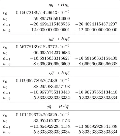
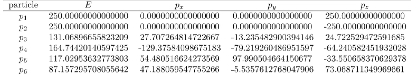
The numerical values of the one-loop amplitudes of the processes (4) in a non-exceptional phase space point are collected in Appendix C. The values of the double and the single poles conform to the universal singular behavior of dimensionally regulated one-loop amplitudes [61–65]. Af- ter appropriate crossing to the H → 4-parton decay kine- matics, we compared our results with the ones presented in Table I of Ref. [26], finding excellent agreement. Fur- thermore, converting our results for the Hjj-production channels from DRED to the ’t Hooft-Veltman scheme, we are in perfect agreement with the most recent version of MCFM (v6.4).

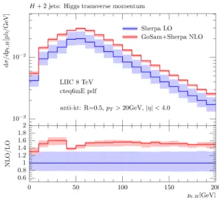
Figure 1: Transverse momentum p

T

of the Higgs boson.

Figure 2: Pseudorapidity η of the Higgs boson.

Figure 3: Transverse momentum p

T

of the first jet.

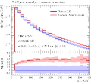
Figure 4: Transverse momentum p

T

of the second jet.

3. Numerical results for pp → H jj

In this section we present a selection of phenomeno- logical results for proton-proton collisions at the LHC at

√ s = 8 TeV, as a sample of the results that can be easily obtained with the GoSam-Sherpa automated setup [37–

40]. A more complete analysis of Higgs production in gluon fusion, which merges several multiplicities [66] and employs the code for the virtual matrix elements of Hjj presented here, is going to be discussed in [67].

The results shown in this section are obtained using the parameters listed below:

M

H

= 125 GeV , G

F

= 1.16639 · 10

⁻⁵

GeV

⁻²

, α

^LO_s

(M

Z

) = 0.129783 , α

^NLO_s

(M

Z

) = 0.117981 , v

²

= 1

√ 2G

F

. (6)

Figure 5: Pseudorapidity η of the first jet.

Figure 6: Pseudorapidity η of the second jet.

We use the CTEQ6L1 and CTEQ6mE [68] parton dis- tribution functions (PDF) for the LO and NLO, respec- tively. The value of the strong coupling at the scale µ is taken from the PDF set starting from the initial values in Eq. (6). The jets are clustered by using the anti-k

T

algo- rithm provided by the FastJet package [69–71] with the following setup:

p

t,j

≥ 20 GeV, | η

j

| ≤ 4.0, R = 0.5 . (7) The Higgs boson is treated as a stable on-shell particle, without including any decay mode. To fix the factorization and the renormalization scale we define

H ˆ

t

= q

M

_H²

+ p

²_t,H

+ X

j

p

t,j

, (8)

where p

t,H

and p

t,j

are the transverse momenta of the

Higgs boson and the jets. The nominal value for the two

scales is defined as

µ = µ

R

= µ

F

= ˆ H

t

, (9)

whereas theoretical uncertainties are assessed by vary- ing simultaneously the factorization and renormalization scales in the range

1

2 H ˆ

t

< µ < 2 ˆ H

t

. (10) The error is estimated by taking the envelope of the re- sulting distributions at the different scales.

3.1. Results

Within our framework, we find the following total cross sections for the process pp → Hjj in gluon fusion:

σ

LO

[pb] = 1.90

^+0.58_−0.41

, σ

NLO

[pb] = 2.90

^+0.05₋0.20

,

where the error is obtained by varying the renormalization and factorization scales as given in Eq. (9). The LO distri- butions have been computed using 2.5 × 10

⁷

phase space points, whereas all NLO distributions have been obtained using 4.0 × 10

⁶

phase space points for the Born and the vir- tual corrections and 5.0 × 10

⁸

points for the real radiation for each scale.

In Figs. 1 and 2, we present the distribution of the trans- verse momentum p

T

of the Higgs boson and its pseudora- pidity η, respectively. Both of them show a K-factor be- tween the LO and the NLO distribution of about 1.5 − 1.6, which is almost flat over a large fraction of kinematical range. Furthermore both plots show a decrease of the scale uncertainty of about 50%. Figures 3 and 4 display the transverse momentum of the first and second jet, whereas their pseudorapidities are shown in Figs. 5 and 6. The previous considerations are also true for these latter plots.

For the transverse momentum distributions, however, we observe a slight change of shapes. In the case of the lead- ing jet, increasing the p

T

, the K-factor decreases from 1.6 to 1.4; while for the second leading jet, it increases from 1.4 to 1.6.

4. Virtual corrections to pp → H jjj

We explore the possibility of extending our framework to the production of a Higgs boson plus three jets at NLO.

The independent partonic processes contributing to Hjjj can be obtained by adding one extra gluon to the final state of the processes listed in Eq.(4). Accordingly, we generate the codes for the virtual corrections to the partonic processes with a quark-pair in the final state,

gg → Hq qg , ¯ q¯ q → Hq qg , ¯ q¯ q → Hq

^′

q ¯

^′

g . (11) The missing channel gg → Hggg, together with the phase space integration, will be discussed in a successive study.

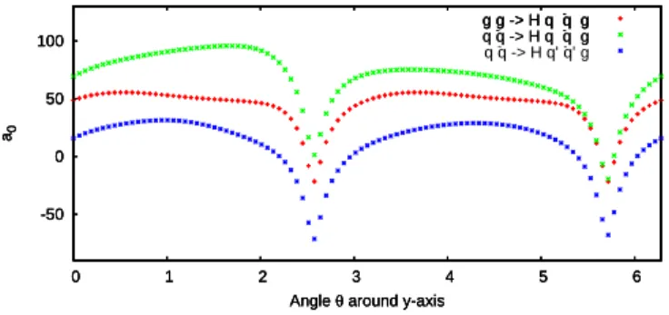
-50 0 50 100

0 1 2 3 4 5 6

a0

Angle θ around y-axis

g g -> H q ^-q g

-50 0 50 100

0 1 2 3 4 5 6

a0

Angle θ around y-axis

g g -> H q ^-q g q ^-q -> H q ^-q g

-50 0 50 100

0 1 2 3 4 5 6

a0

Angle θ around y-axis

g g -> H q ^-q g q ^-q -> H q ^-q g q ^-q -> H q’ ^-q’ g

Figure 7: Finite-term of the virtual matrix-elements for gg → Hq qg ¯ (red), q¯ q → Hq qg ¯ (green), q¯ q → Hq

^′

q ¯

^′

g (blue).

We compute, for the first time, the virtual matrix ele- ments for the three subprocesses listed above, and show their results along a certain one-dimensional curve in the space of final state momenta. We take the initial partons to have momentum p

1

and p

2

, whose 3-momenta lie along the z-axis, and choose an arbitrary point for the final state momenta { p

3

, p

4

, p

5

, p

6

} . For simplicity, we start with the same phase space point used in the Appendix D (see Ta- ble D.4). Then, we create new momentum configurations by rotating the final state through an angle θ about the y-axis. Figure 7 displays the behavior of the finite part a

0

of the individual 2 → 4 amplitudes defined as 2 Re {M

^{tree-level∗}

M

^one-loop

}

(4πα

s

) |M

^tree-level

|

²

≡ a

₋2

ǫ

²

+ a

₋1

ǫ + a

0

, (12) when the final external momenta are rotated from θ = 0 to θ = 2π. The plots are obtained by sampling over 100 points.

Numerical values for the one-loop amplitudes of the pro- cesses listed in (11) are collected in Appendix D.

Also in this case we verify that the values of the dou- ble and the single poles conform to the universal singu- lar behavior of dimensionally regulated one-loop ampli- tudes [65].

5. Conclusions

We presented the calculation of the associated produc- tion of a Higgs boson and two jets, pp → Hjj, at NLO in QCD, employing the infinite top-mass approximation.

The results were obtained by using a fully automated framework for fixed order NLO QCD calculations based on the interplay of the packages GoSam and Sherpa, in- terfaced through the BLHA standards. We discussed the technical aspects of the computation, and showed the nu- merical impact of the radiative corrections on the distribu- tion of the transverse momentum of the Higgs boson and its pseudorapidity, as well as of the transverse momentum and pseudorapidity of the leading and second leading jet.

All plots show a K-factor between the LO and the NLO

distributions of about 1.5, over a large fraction of kine- matical range, and a decrease of the scale uncertainty of about 50%.

The evaluation of the virtual corrections constitutes an application of the d-dimensional integrand reduction to theories with higher dimensional operators.

Finally, as an initial step towards the evaluation of pp → Hjjj at NLO, we presented first results for the one-loop matrix elements of the partonic processes with a quark- pair in the final state.

Acknowledgements

We thank the Sherpa collaboration for encouraging and stimulating discussions and feedback on the manuscript.

We also would like to thank Thomas Hahn for his tech- nical support while structuring the computing resources needed by our codes, and Joscha Reichel for feedback on the extended-rank version of samurai.

The work of H.v.D., G.L., P.M., and T.P. was supported by the Alexander von Humboldt Foundation, in the frame- work of the Sofja Kovaleskaja Award Project “Advanced Mathematical Methods for Particle Physics”, endowed by the German Federal Ministry of Education and Research.

G.O. was supported in part by the National Science Foundation under Grant PHY-1068550.

H.v.D. and G.L. thank the Center for Theoretical Physics of New York City College of Technology for hos- pitality during the final stages of this project.

The Feynman diagrams present in this paper are drawn using FeynArts [72].

Appendix A. Effective Higgs-gluon vertices The operator L in Eq. (1) describes the gluon-Higgs in- teraction in the large top-mass limit and leads to the fol- lowing set of Feynman rules:

H g

1

g

2

= − ig

eff

F

c^µ₁¹,c^µ₂²

H g

3

g

1

g

2

= g

eff

g

s

F

c^µ1¹,c^µ2²,c^µ33

H g

2

g

3

g

1

g

4

= ig

eff

g

_s²

F

c^µ₁¹,c^µ₂²,c^µ3₃^µ,c⁴₄

where we define

F

c^µ1¹,c^µ2²

= δ

c1c2

(p

^µ₁²

p

^µ₂¹

− p

1

· p

2

g

^µ1µ2

) , F

c^µ₁¹,c^µ₂²,c^µ3₃

= f

c1c2c3

g

^µ1µ2

(p

^µ1³

− p

^µ₂³

) + g

^µ2µ3

(p

^µ₂¹

− p

^µ₃¹

)

+ g

^µ3µ1

(p

^µ₃²

− p

^µ₁²

) ,

F

c^µ₁¹,c^µ₂²,c^µ3₃^µ,c⁴₄

= f

c1c2i

f

c3c4i

[ g

^µ1µ4

g

^µ2µ3

− g

^µ1µ3

g

^µ2µ4

] + f

c₁c₃i

f

c₂c₄i

[ g

^µ1µ4

g

^µ2µ3

− g

^µ1µ2

g

^µ3µ4

] + f

c1c4i

f

c2c3i

[ g

^µ1µ3

g

^µ2µ4

− g

^µ1µ2

g

^µ3µ4

].

(A.1) In Eq. (A.1) sum over repeated indices is understood.

Appendix B. Higher-rank integrands

Higher-rank integrands, i.e. integrands where the pow- ers of loop momenta in the numerator is higher than the numbers of denominators, are present in diagrams with a Higgs boson coupled to a purely gluonic loop involving only three-gluon vertices. The generic numerator Γ

^ε1···εn

of a (n + 1)-denominator one-loop diagram can be written as

Γ

^ε1···εn

≡ F

^µ1µ₂

G

^{µ1µ2ε1···εn}

, (B.1) where F

^µ1µ2

is the Hgg vertex defined in Eq. (A.1), and G

^{µ1µ2ε1···εn}

is the numerator of an (n + 2)-gluon tree-level diagram, which can be represented by

ε

2

ε

1

ε

n

≡

µ

2

µ

1

q µ

2

µ

1

ε

2

ε

1

ε

n

q

We are interested in the leading behaviour in q of Γ

^ε1···εn

, and we want to show that the highest-rank terms, with rank r = n + 2, are proportional to the loop momentum squared, q

²

. In order to show it, we neglect all external momenta and all the terms proportional to q

²

.

From Eq. (A.1), one trivially has

F

µ1µ2

= q

µ1

q

µ2

+ O (q

²

) , (B.2) while the generic tensor structure of G

^{µ1µ2ε1···εn}

is

G

^{µ1µ2ε1···εn}

= q

^µ1

T

1^{µ2ε1···εn}

+ q

^µ2

T

2^{µ1ε1···εn}

+ + g

^µ1µ2

T

g^ε1···εn

+ O (q

²

) , (B.3) where T

¹

, T

²

, and T

^g

are tensors which may depend on q as well. Indeed Eq. (B.3) is fulfilled for n = 0, 1,

G

^µ1µ2

= g

^µ1µ2

G

^µ1µ2ε1

= g

^µ1ε1

q

^µ2

+ g

^µ2ε1

q

^µ1

− 2g

^µ2µ1

q

^ε1

, (B.4)

while for n > 1 it can be proven by induction over n by using

G

^{µ1µ2ε1···εn}

= G

µ^{µ2ε1···εn−1}

G

^µ1µεn

, (B.5) that is

≡ ε

1

ε

2

ε

n

µ

2

q µ

1

ε

1

ε

2

ε

n−1

µ

2

µ q

ε

n

µ

1

µ

Combining Eq. (B.2) and Eq. (B.3), it is easy to realize that each rank-(n + 2) term of an n + 1-denominator dia- gram Γ

^ε1···εn

is proportional to q

²

. The factor q

²

simplifies against one denominator leading to a rank n numerator of an n-denominator integrand.

Appendix C. Benchmark points for pp → H jj In this appendix we provide numerical results for the renormalized virtual contributions to the processes (4), in correspondence with the phase space point in Table C.1.

The parameters can be read from Eqs. (6), while the renor- malization and factorization scales are set to the Higgs mass value. The assignment of the momenta proceeds as follows

g(p

1

) g(p

2

) → H(p

3

) g(p

4

) g(p

5

) , g(p

1

) g(p

2

) → H(p

3

) q(p

4

) ¯ q(p

5

) , q(p

1

) ¯ q(p

2

) → H(p

3

) q(p

4

) ¯ q(p

5

) ,

q(p

1

) ¯ q(p

2

) → H(p

3

) q

^′

(p

4

) ¯ q

^′

(p

5

) . (C.1) The results are collected in Table C.2 and are computed using DRED. In the second column of the table we provide the LO squared amplitude,

c

0

≡ |M

^tree-level

|

²

(4πα

s

)

²

g

²_eff

, (C.2)

and the coefficients a

i

defined in Eq. (12). As a check on the reconstruction of the renormalized poles, in the last column we show the values of a

₋1

and a

₋2

obtained by the universal singular behavior of the dimensionally regularized one-loop amplitudes [65].

Appendix D. Benchmark points for pp → H jjj In this appendix we collect first numerical results for the renormalized virtual contributions to

g(p

1

) g(p

2

) → H (p

3

) q(p

4

) ¯ q(p

5

) g(p

6

) , q(p

1

) ¯ q(p

2

) → H (p

3

) q(p

4

) ¯ q(p

5

) g(p

6

) ,

q(p

1

) ¯ q(p

2

) → H (p

3

) q

^′

(p

4

) ¯ q

^′

(p

5

) g(p

6

) . (D.1)

gg → Hgg c

0

0.1507218951429643 · 10

⁻³

a

0

59.8657965614009

a

₋1

− 26.4694115468536 − 26.46941154671207 a

₋2

− 12.00000000000001 − 12.00000000000000

gg → Hq q ¯ c

0

0.5677813961826772 · 10

⁻⁶

a

0

66.6635142370683

a

₋1

− 16.5816633315627 − 16.58166333155405 a

₋2

− 8.66666666666669 − 8.666666666666668

q¯ q → Hq q ¯ c

0

0.1099527895267439 · 10

⁻⁵

a

0

88.2959834057198

a

₋1

− 10.9673755313443 − 10.96737553134440 a

₋2

− 5.33333333333332 − 5.333333333333334

q¯ q → Hq

^′

q ¯

^′

c

0

0.1011096724203529 · 10

⁻⁶

a

0

33.9521626734153

a

₋1

− 13.8649292834138 − 13.86492928341388 a

₋2

− 5.33333333333334 − 5.333333333333334

Table C.2: Numerical results for the processes listed in Eq. (C.1)

gg → Hq qg ¯ b

0

0.6309159660038877 · 10

⁻⁴

a

0

48.68424097859422

a

₋1

− 36.08277727147958 − 36.08277728199094 a

₋2

− 11.66666666667209 − 11.66666666666667

q q ¯ → Hq qg ¯ b

0

0.3609139855530763 · 10

⁻⁴

a

0

69.32351140490162

a

₋1

− 29.98862932963380 − 29.98862932963629 a

₋2

− 8.333333333333339 − 8.333333333333334

q¯ q → Hq

^′

q ¯

^′

g b

0

0.2687990772405433 · 10

⁻⁵

a

0

15.79262767177915

a

₋1

− 32.35320587070861 − 32.35320587073038 a

₋2

− 8.333333333333398 − 8.333333333333332

Table D.3: Numerical results for the processes listed in Eq. (D.1)

The results, collected in Table D.3, have been computed

using the parameters in Eqs. (6), with the renormalization

and factorization scales set to the Higgs mass value, and

choosing the phase space point given in Table D.4. In

particular, in the second column of Table D.3, we provide

particle E p

x

p

y

p

z

p

1

250.00000000000000 0.0000000000000000 0.0000000000000000 250.00000000000000 p

2

250.00000000000000 0.0000000000000000 0.0000000000000000 -250.00000000000000 p

3

143.67785106160801 51.663364918413812 -22.547134012261804 42.905108772983255 p

4

190.20318863787611 -153.36110830475005 -108.23578590696623 -30.702411577195452 p

5

166.11896030051594 101.69774338633616 130.78291991922802 -12.202697195787838

Table C.1: Benchmark phase space point for Higgs plus two jets production

particle E p

x

p

y

p

z

p

1

250.00000000000000 0.0000000000000000 0.0000000000000000 250.00000000000000 p

2

250.00000000000000 0.0000000000000000 0.0000000000000000 -250.00000000000000 p

3

131.06896655823209 27.707264814722667 -13.235482900394146 24.722529472591685 p

4

164.74420140597425 -129.37584098675183 -79.219260486951597 -64.240582451932028 p

5

117.02953632773803 54.480516624273569 97.990504664150677 -33.550658370629378 p

6

87.157295708055642 47.188059547755266 -5.5357612768047906 73.068711349969661

Table D.4: Benchmark phase space point for Higgs plus three jets production

the quantity b

0

, b

0

≡ |M

^tree-level

|

²

(4πα

s

)

³

g

²_eff

, (D.2)

and the coefficients a

i

defined in Eq. (12). In the third column we show the values of a

₋1

and a

₋2

obtained from the universal singular behavior of one-loop amplitudes.

References

[1] ATLAS Collaboration Collaboration, G. Aad et al.,

“Observation of a new particle in the search for the Standard Model Higgs boson with the ATLAS detector at the LHC,”

Phys.Lett. B716 (2012) 1–29, 1207.7214.

[2] CMS Collaboration Collaboration, S. Chatrchyan et al.,

“Observation of a new boson at a mass of 125 GeV with the CMS experiment at the LHC,” Phys.Lett. B716 (2012) 30–61, 1207.7235.

[3] J. M. Campbell, R. K. Ellis, and G. Zanderighi,

“Next-to-Leading order Higgs + 2 jet production via gluon fusion,” JHEP 0610 (2006) 028, hep-ph/0608194.

[4] J. M. Campbell, R. Ellis, and C. Williams, “Hadronic production of a Higgs boson and two jets at next-to-leading order,” Phys.Rev. D81 (2010) 074023, 1001.4495.

[5] V. Del Duca, W. Kilgore, C. Oleari, C. Schmidt, and D. Zeppenfeld, “Higgs + 2 jets via gluon fusion,”

Phys.Rev.Lett. 87 (2001) 122001, hep-ph/0105129.

[6] V. Del Duca, W. Kilgore, C. Oleari, C. Schmidt, and D. Zeppenfeld, “Gluon fusion contributions to H + 2 jet production,” Nucl.Phys. B616 (2001) 367–399,

hep-ph/0108030.

[7] F. Wilczek, “Decays of Heavy Vector Mesons Into Higgs Particles,” Phys.Rev.Lett. 39 (1977) 1304.

[8] S. Dawson, “Radiative corrections to Higgs boson production,” Nucl.Phys. B359 (1991) 283–300.

[9] A. Djouadi, M. Spira, and P. Zerwas, “Production of Higgs bosons in proton colliders: QCD corrections,” Phys.Lett.

B264 (1991) 440–446.

[10] R. V. Harlander and W. B. Kilgore, “Next-to-next-to-leading order Higgs production at hadron colliders,” Phys.Rev.Lett. 88 (2002) 201801, hep-ph/0201206.

[11] C. Anastasiou and K. Melnikov, “Higgs boson production at hadron colliders in NNLO QCD,” Nucl.Phys. B646 (2002) 220–256, hep-ph/0207004.

[12] V. Ravindran, J. Smith, and W. L. van Neerven, “NNLO corrections to the total cross-section for Higgs boson production in hadron hadron collisions,” Nucl.Phys. B665 (2003) 325–366, hep-ph/0302135.

[13] C. Anastasiou, K. Melnikov, and F. Petriello, “Fully differential Higgs boson production and the di-photon signal through next-to-next-to-leading order,” Nucl.Phys. B724 (2005) 197–246, hep-ph/0501130.

[14] C. Anastasiou, G. Dissertori, and F. Stockli, “NNLO QCD predictions for the H → W W → lνlν signal at the LHC,”

JHEP 0709 (2007) 018, 0707.2373.

[15] S. Catani and M. Grazzini, “An NNLO subtraction formalism in hadron collisions and its application to Higgs boson production at the LHC,” Phys.Rev.Lett. 98 (2007) 222002, hep-ph/0703012.

[16] M. Grazzini, “NNLO predictions for the Higgs boson signal in the H → W W → lνlν and H → ZZ → 4l decay channels,”

JHEP 0802 (2008) 043, 0801.3232.

[17] C. R. Schmidt, “H → g g g (g q anti-q) at two loops in the large M(t) limit,” Phys.Lett. B413 (1997) 391–395, hep-ph/9707448.

[18] D. de Florian, M. Grazzini, and Z. Kunszt, “Higgs production with large transverse momentum in hadronic collisions at next-to-leading order,” Phys.Rev.Lett. 82 (1999) 5209–5212, hep-ph/9902483.

[19] V. Ravindran, J. Smith, and W. Van Neerven,

“Next-to-leading order QCD corrections to differential distributions of Higgs boson production in hadron hadron collisions,” Nucl.Phys. B634 (2002) 247–290, hep-ph/0201114.

[20] C. J. Glosser and C. R. Schmidt, “Next-to-leading corrections to the Higgs boson transverse momentum spectrum in gluon fusion,” JHEP 0212 (2002) 016, hep-ph/0209248.

[21] S. Dawson and R. Kauffman, “Higgs boson plus multi - jet rates at the SSC,” Phys.Rev.Lett. 68 (1992) 2273–2276.

[22] R. P. Kauffman, S. V. Desai, and D. Risal, “Production of a Higgs boson plus two jets in hadronic collisions,” Phys.Rev.

D55 (1997) 4005–4015, hep-ph/9610541.

[23] V. Del Duca, A. Frizzo, and F. Maltoni, “Higgs boson production in association with three jets,” JHEP 0405 (2004) 064, hep-ph/0404013.

[24] L. J. Dixon, E. N. Glover, and V. V. Khoze, “MHV rules for Higgs plus multi-gluon amplitudes,” JHEP 0412 (2004) 015, hep-th/0411092.

[25] S. Badger, E. N. Glover, and V. V. Khoze, “MHV rules for Higgs plus multi-parton amplitudes,” JHEP 0503 (2005) 023, hep-th/0412275.

[26] R. K. Ellis, W. Giele, and G. Zanderighi, “Virtual QCD

corrections to Higgs boson plus four parton processes,”

Phys.Rev. D72 (2005) 054018, hep-ph/0506196.

[27] R. K. Ellis, W. Giele, and G. Zanderighi, “Semi-numerical evaluation of one-loop corrections,” Phys.Rev. D73 (2006) 014027, hep-ph/0508308.

[28] C. F. Berger, V. Del Duca, and L. J. Dixon, “Recursive Construction of Higgs-Plus-Multiparton Loop Amplitudes:

The Last of the Phi-nite Loop Amplitudes,” Phys.Rev. D74 (2006) 094021, hep-ph/0608180.

[29] S. Badger and E. N. Glover, “One-loop helicity amplitudes for H → gluons: The All-minus configuration,”

Nucl.Phys.Proc.Suppl. 160 (2006) 71–75, hep-ph/0607139.

[30] S. Badger, E. N. Glover, and K. Risager, “One-loop phi-MHV amplitudes using the unitarity bootstrap,” JHEP 0707 (2007) 066, 0704.3914.

[31] E. N. Glover, P. Mastrolia, and C. Williams, “One-loop phi-MHV amplitudes using the unitarity bootstrap: The General helicity case,” JHEP 0808 (2008) 017, 0804.4149.

[32] S. Badger, E. Nigel Glover, P. Mastrolia, and C. Williams,

“One-loop Higgs plus four gluon amplitudes: Full analytic results,” JHEP 1001 (2010) 036, 0909.4475.

[33] L. J. Dixon and Y. Sofianatos, “Analytic one-loop amplitudes for a Higgs boson plus four partons,” JHEP 0908 (2009) 058, 0906.0008.

[34] S. Badger, J. M. Campbell, R. K. Ellis, and C. Williams,

“Analytic results for the one-loop NMHV Hqqgg amplitude,”

JHEP 0912 (2009) 035, 0910.4481.

[35] J. M. Campbell, R. K. Ellis, R. Frederix, P. Nason, C. Oleari, et al., “NLO Higgs Boson Production Plus One and Two Jets Using the POWHEG BOX, MadGraph4 and MCFM,” JHEP 1207 (2012) 092, 1202.5475.

[36] T. Binoth, F. Boudjema, G. Dissertori, A. Lazopoulos, A. Denner, et al., “A Proposal for a standard interface between Monte Carlo tools and one-loop programs,”

Comput.Phys.Commun. 181 (2010) 1612–1622, 1001.1307.

Dedicated to the memory of, and in tribute to, Thomas Binoth, who led the effort to develop this proposal for Les Houches 2009.

[37] G. Cullen, N. Greiner, G. Heinrich, G. Luisoni, P. Mastrolia, et al., “Automated One-Loop Calculations with GoSam,”

Eur.Phys.J. C72 (2012) 1889, 1111.2034.

[38] T. Gleisberg, S. Hoeche, F. Krauss, M. Schonherr,

S. Schumann, et al., “Event generation with SHERPA 1.1,”

JHEP 0902 (2009) 007, 0811.4622.

[39] G. Luisoni, M. Sch¨ onherr, and F. Tramontano , in preparation.

[40] http://gosam.hepforge.org/proc/.

[41] G. Ossola, C. G. Papadopoulos, and R. Pittau, “Reducing full one-loop amplitudes to scalar integrals at the integrand level,”

Nucl.Phys. B763 (2007) 147–169, hep-ph/0609007.

[42] G. Ossola, C. G. Papadopoulos, and R. Pittau, “Numerical evaluation of six-photon amplitudes,” JHEP 0707 (2007) 085, 0704.1271.

[43] R. K. Ellis, W. T. Giele, and Z. Kunszt, “A Numerical Unitarity Formalism for Evaluating One-Loop Amplitudes,”

JHEP 03 (2008) 003, 0708.2398.

[44] W. T. Giele, Z. Kunszt, and K. Melnikov, “Full one-loop amplitudes from tree amplitudes,” JHEP 0804 (2008) 049, 0801.2237.

[45] P. Mastrolia, G. Ossola, T. Reiter, and F. Tramontano,

“Scattering AMplitudes from Unitarity-based Reduction Algorithm at the Integrand-level,” JHEP 1008 (2010) 080, 1006.0710.

[46] P. Mastrolia, E. Mirabella, G. Ossola, and T. Peraro,

“Scattering Amplitudes from Multivariate Polynomial Division,” Phys.Lett. B718 (2012) 173–177, 1205.7087.

[47] P. Mastrolia, E. Mirabella, and T. Peraro, “Integrand reduction of one-loop scattering amplitudes through Laurent series expansion,” 1203.0291.

[48] P. Nogueira, “Automatic Feynman graph generation,”

J.Comput.Phys. 105 (1993) 279–289.

[49] J. A. M. Vermaseren, “New features of FORM,”

math-ph/0010025.

[50] T. Reiter, “Optimising Code Generation with haggies,”

Comput.Phys.Commun. 181 (2010) 1301–1331, 0907.3714.

[51] G. Cullen, M. Koch-Janusz, and T. Reiter, “Spinney: A Form Library for Helicity Spinors,” Comput.Phys.Commun. 182 (2011) 2368–2387, 1008.0803.

[52] G. Ossola, C. G. Papadopoulos, and R. Pittau, “On the Rational Terms of the one-loop amplitudes,” JHEP 0805 (2008) 004, 0802.1876.

[53] P. Mastrolia, G. Ossola, C. Papadopoulos, and R. Pittau,

“Optimizing the Reduction of One-Loop Amplitudes,” JHEP 0806 (2008) 030, 0803.3964.

[54] G. Heinrich, G. Ossola, T. Reiter, and F. Tramontano,

“Tensorial Reconstruction at the Integrand Level,” JHEP 1010 (2010) 105, 1008.2441.

[55] G. van Oldenborgh, “FF: A Package to evaluate one loop Feynman diagrams,” Comput.Phys.Commun. 66 (1991) 1–15.

[56] R. K. Ellis and G. Zanderighi, “Scalar one-loop integrals for QCD,” JHEP 02 (2008) 002, 0712.1851.

[57] A. van Hameren, “OneLOop: For the evaluation of one-loop scalar functions,” Comput.Phys.Commun. 182 (2011) 2427–2438, 1007.4716.

[58] G. Cullen, J. Guillet, G. Heinrich, T. Kleinschmidt, E. Pilon, et al., “Golem95C: A library for one-loop integrals with complex masses,” Comput.Phys.Commun. 182 (2011) 2276–2284, 1101.5595.

[59] F. Krauss, R. Kuhn, and G. Soff, “AMEGIC++ 1.0: A Matrix element generator in C++,” JHEP 0202 (2002) 044,

hep-ph/0109036.

[60] T. Gleisberg and F. Krauss, “Automating dipole subtraction for QCD NLO calculations,” Eur.Phys.J. C53 (2008) 501–523, 0709.2881.

[61] W. Giele and E. N. Glover, “Higher order corrections to jet cross-sections in e+ e- annihilation,” Phys.Rev. D46 (1992) 1980–2010.

[62] Z. Kunszt, A. Signer, and Z. Trocsanyi, “Singular terms of helicity amplitudes at one loop in QCD and the soft limit of the cross-sections of multiparton processes,” Nucl.Phys. B420 (1994) 550–564, hep-ph/9401294.

[63] S. Catani and M. Seymour, “The Dipole formalism for the calculation of QCD jet cross-sections at next-to-leading order,” Phys.Lett. B378 (1996) 287–301, hep-ph/9602277.

[64] S. Catani and M. Seymour, “A General algorithm for

calculating jet cross-sections in NLO QCD,” Nucl.Phys. B485 (1997) 291–419, hep-ph/9605323.

[65] S. Catani, S. Dittmaier, and Z. Trocsanyi, “One loop singular behavior of QCD and SUSY QCD amplitudes with massive partons,” Phys.Lett. B500 (2001) 149–160, hep-ph/0011222.

[66] S. Hoeche, F. Krauss, M. Schonherr, and F. Siegert, “QCD matrix elements + parton showers: The NLO case,”

1207.5030.

[67] Sherpa collaboration, in preparation.

[68] J. Pumplin, D. Stump, J. Huston, H. Lai, P. M. Nadolsky, et al., “New generation of parton distributions with uncertainties from global QCD analysis,” JHEP 0207 (2002) 012,

hep-ph/0201195.

[69] M. Cacciari and G. P. Salam, “Dispelling the N

³

myth for the k

^t

jet-finder,” Phys.Lett. B641 (2006) 57–61, hep-ph/0512210.

[70] M. Cacciari, G. P. Salam, and G. Soyez, “The Anti-k(t) jet clustering algorithm,” JHEP 0804 (2008) 063, 0802.1189.

[71] M. Cacciari, G. P. Salam, and G. Soyez, “FastJet User Manual,” Eur.Phys.J. C72 (2012) 1896, 1111.6097.

[72] T. Hahn, “Generating Feynman diagrams and amplitudes with

FeynArts 3,” Comput.Phys.Commun. 140 (2001) 418–431,

hep-ph/0012260.