Performance of large-R jets and jet substructure reconstruction with the ATLAS detector

ATLAS-CONF-2012-065 04July2012

ATLAS NOTE

ATLAS-CONF-2012-065

June 26, 2012

Performance of large-R jets and jet substructure reconstruction with the ATLAS detector

The ATLAS Collaboration

Abstract

This paper presents the application of techniques to study jet substructure. The per- formance of modified jet algorithms for a variety of jet types and event topologies is in- vestigated. Properties of jets subjected to the mass-drop filtering, trimming and pruning algorithms are found to have a reduced sensitivity to multiple proton-proton interactions and exhibit improved stability at high luminosity. Monte Carlo studies of the signal-background discrimination with jet grooming in new physics searches based on jet invariant mass and jet substructure properties are also presented. The application of jet trimming is shown to improve the robustness of large-Rjet measurements, reduce sensitivity to the superfluous effects due to the intense environment of the high luminosity LHC, and improve the physics potential of searches for heavy boosted objects. The analyses presented in this note use the full 2011 ATLAS dataset, corresponding to an integrated luminosity of 4.7±0.2 fb⁻¹.

c

Copyright 2012 CERN for the benefit of the ATLAS Collaboration.

Reproduction of this article or parts of it is allowed as specified in the CC-BY-3.0 license.

1 Introduction

Jets have historically been utilized at high energy colliders as proxies for the quarks and gluons produced in the primary collisions. With the high-luminosity conditions at the LHC, soft particles unrelated to the hard scattering contaminate jets in the detector considerably more than at previous experiments, making it more di

ffi

cult to resolve the particles originating from the hard interaction. This is especially true for boosted objects whose decay products may be sufficiently collimated such that standard reconstruction techniques begin to fail. In events where such decays are fully contained within individual large-radius jets, a diminished mass resolution due to the high luminosity environment weakens the sensitivity to new physics processes.

One example of a new physics process which may produce heavy objects with a significant Lorentz boost is the decay of a new heavy gauge boson, the Z

⁰

, to top quark pairs. Figure

1

shows the true angular separation between the W and b decay products of a top quark in simulated Z

⁰ →

t¯ t (m

Z⁰ =

1.6 TeV) events, as well as the separation between the light quarks of the subsequent hadronically-decaying W. In each case, the angular separation of the decay products is approximately

∆

R

≈

2m

p

_T,

(1)

where

∆

R

= p

(

∆y)²+

(

∆φ)²

, and p

_T

and m are the transverse momentum and mass of the decaying particle, respectively

¹

. For p

^W_T >

200 GeV, the ability to resolve the individual hadronic decay products using standard narrow-cone jet algorithms begins to degrade, and above p

^top_T >

350 GeV, the decay products of the top quark tend to have a separation

∆

R

<

1.0. Techniques designed to recover sensitivity in such cases focus on large-R jets in order to maximize efficiency

²

. At

√

s

=

7 TeV, nearly one thousand Standard Model t¯ t events per fb

⁻¹

are expected in this momentum regime. It is in this region of phase space, which was limited by statistics and the available energy at previous colliders, where new physics may appear.

A single jet that contains all of the decay products of a massive particle will have significantly dif- ferent properties than a single jet of the same p

_T

originating from a single light-quark or gluon. The characteristic two-body or three-body decays of a vector boson or top quark result in a hard substructure that is absent from the light-quark and gluon jets, and this can be more clearly resolved by removing soft radiation from jets. This selective removal of soft radiation during the process of iterative recombination in jet reconstruction is generally referred to as jet “grooming”.

Recently many jet grooming algorithms have been designed to remove contributions to a given jet that are irrelevant or detrimental to resolving the hard decay products from a boosted object. The struc- tural differences between jets formed from light quarks or gluons and individual jets originating from a boosted hadronic particle decay form the basis for these tools. Consequently, the characteristic sub- structure within such a jet is retained while reducing the impact of the fluctuations of the parton shower and underlying event (UE), and mitigating the influence of pile-up (additional pp collisions apart from the primary hard collision in an event). Thus, a groomed jet can also be a powerful tool to discrimi- nate between the dominant multi-jet background and the heavy particle decay, thereby increasing signal sensitivity.

1The ATLAS coordinate system is a right-handed system with thex-axis pointing to the center of the LHC ring and the y-axis pointing upwards. The polar angleθis measured with respect to the LHC beam-line. The azimuthal angleφis measured with respect to the x-axis. The rapidity is defined asy =0.5×ln[(E+pz)/(E−pz)], whereEdenotes the energy and pz is the component of the momentum along the beam direction. The pseudorapidityηis an approximation for rapidityyin the high energy limit, and it is related to the polar angleθasη =−ln tan₂^θ. Transverse momentum and energy are defined as pT=p×sinθandET=E×sinθ, respectively.

2In this paper, “large-R” refers to jets with a distance parameterR≥1.0

1

100 200 300 400 500 600 700 800 900 0

0.2 0.4 0.6 0.8 1 1.2 1.4 1.6 1.8 2

[GeV]

top p

100 200 300 400 500 600 700 800 900

R (W ,b ) ∆

0.2 0 0.4 0.6 0.8 1 1.2 1.4 1.6 1.8 2

0 50 100 150 200 250

[GeV]

top pT

0 100 200 300 400 500 600 700 800 900

R(W,b)∆

0 0.2 0.4 0.6 0.8 1 1.2 1.4 1.6 1.8 2 2.2

→ Wb , t t

→ t Pythia Z’

ATLAS Preliminary - Simulation

(a) t→Wb

100 200 300 400 500 600 700 800 0

0.5 1 1.5

2 2.5 3 3.5 4

[GeV]

100 200 300 W p 400 500 600 700 800

) q R(q, ∆

0 0.5 1 1.5

2 2.5 3 3.5 4

0 50 100 150 200 250

[GeV]

W pT

0 100 200 300 400 500 600 700 800

)q R(q,∆

0 0.5 1 1.5

2 2.5 3 3.5 4

→ Wb , t t

→ t Pythia Z’

ATLAS Preliminary - Simulation

(b)W→q¯q

Figure 1:

(a)

The opening angle between the W and b in top decays, t

→

Wb, as a function of the top p

_T

in simulated PYTHIA Z

⁰ →

t¯ t (m

Z⁰ =

1.6 TeV) events.

(b)

The opening angle of the W

→

q q ¯ system from t

→

Wb decays as a function of the W p

_T

. Both distributions are at the particle level.

This note presents the results of a comprehensive study of the performance of jet grooming algo- rithms using the 2011 ATLAS dataset corresponding to an integrated luminosity of (4.7

±

0.2) fb

⁻¹

. Three jet grooming techniques are studied: mass-drop filtering, trimming, and pruning. These tech- niques utilize the internal structure of the jet in order to reduce the sensitivity to pile-up and UE, as well as improve jet mass resolution.

Measurements of groomed jet properties in the presence of pile-up (along with a companion study [1]) are made for jets across a wide range of jet transverse momentum ( p

^jet_T

). Comparisons are made to generators incorporating leading-order (LO), e.g. PYTHIA [2] and next-to-leading-order (NLO), e.g.

POWHEG [3,4] matrix elements, interfaced to PYTHIA for parton showering and hadronization, as well as to GEANT4 for full detector simulation.

Section

2

describes the design and implementation of the grooming algorithms used in ATLAS, as well as the definitions of the various substructure observables discussed throughout the text. The data samples and Monte Carlo simulation used for comparison are introduced in Section

3. The performance

and validation of jet calibrations for large-R and groomed jets described in Section

4

provide the starting point necessary to establish the use of these new jet algorithms in physics analyses. Data to MC compar- isons are then discussed in Section

5

for the jet substructure observables introduced in Section

2. Finally,

Section

6

presents comparisons of grooming algorithms applied to multiple QCD jet events and a sample selected to contain high p

_T

hadronically-decaying top quarks in data.

2 Jet Grooming Algorithms and Substructure Observables in ATLAS

This section describes jet reconstruction algorithms and presents three jet algorithm modification pro-

cedures studied in ATLAS, referred to as jet “grooming.” Mass-drop filtering, trimming, and pruning

are described and performance measures related to each are defined. The different configurations of the

grooming algorithms described in this section are summarized in Table

1. Additionally, a technique to

tag boosted top quarks using the mass-drop/filtering method is introduced.

2.1 Inputs to jet reconstruction

The inputs to jet reconstruction, or “proto-jets”, are either stable particles with a lifetime of at least 10 ps (excluding muons and neutrinos) in the case of MC “truth jets”, charged particle tracks in the case of so-called “track jets” [5], or three-dimensional topo-clusters [6] in the case of fully reconstructed calorimeter jets. In the reconstruction of track jets, track quality selection is applied in order to ensure good quality tracks that originate from the primary reconstructed vertex which has the largest

P

(p

_T^track

)

²

in the event and contains at least two tracks. The selection criteria are:

•

Transverse momentum: p

^track_T >

0.5 GeV;

•

Transverse impact parameter:

|d₀|<

1.0 mm;

•

Longitudinal impact parameter:

|z₀| ×

sin(θ)

<

1.0 mm;

•

Silicon detector hits on tracks: N

_Pixel≥

1, N

_SCT≥

6;

where the impact parameters are computed with respect to the primary vertex, and

θ

is the angle between the track and the beam. In the reconstruction of calorimeter jets, calorimeter cells are clustered together using a topological clustering algorithm. These objects provide a three-dimensional representation of energy depositions in the calorimeter with a nearest neighbor noise suppression algorithm. The resulting topo-clusters are then classified as either electromagnetic or hadronic based on their shape, depth and energy density. Energy corrections are then applied in order to calibrate the clusters to the hadronic scale.

2.2 Jet algorithms

Three jet algorithms are studied here: the anti-k

t

algorithm [7], the Cambridge-Aachen (C/A) algo- rithm [8,

9], and the

k

t

algorithm [10,

11]. These algorithms are implemented within the framework of

the FastJet software [12,

13]. They represent the most widely used infrared and collinear-safe jet algo-

rithms available for hadron-hadron collider physics today. Furthermore, in the case of the k

_t

and C/A algorithms, the clustering history of the algorithm – that is, the ordering and structure of the pair-wise recombinations made during jet reconstruction – provides spatial and kinematic information about the anatomy of that jet. The anti-k

t

algorithm provides stable, robust jets that are defined primarily by the highest-p

_T

constituent. The compromise is that the structure of the jet as defined by the anti-k

t

algorithm carries little or no information about the ordering of the shower or wide angular-scale structure. It is, however, possible to exploit this stability and recover meaningful information about the jet substructure:

anti-k

t

jets are selected for analysis based on their kinematics (η and p

_T

), and then the jet constituents are reclustered with the k

t

algorithm to enable use of the k

t

-ordered splitting scales described in Sec- tion

2.3. The four-momentum recombination scheme is used in all cases and the jet finding is performed

in rapidity-azimuthal angle (y-φ) coordinates. Jet selections and corrections are made in pseudorapidity- azimuthal angle (η-φ) coordinates.

The iterative recombination procedure works by first creating a list of all objects (either hadrons, topo-clustersor tracks) in an event. The ordering of the list is irrelevant, and proto-jets are formed from these objects. Two distance measures in

y-φ-space are associated to each member of the list, between the

proto-jet and its closest neighbor (as defined in Eq.

2) and between the proto-jet and the beam (Eq.3).

ρi j =

min

p

^2p_{T i},

p

^2p_{T j}

(∆ R

i j

)

²

R

² .

(2)

ρiB=

p

^2p_{T i}

(3)

3

Here, p

_{T i}

is the transverse momentum of the proto-jet, p is an integer,

∆

R

_{i j} = q

(y

i−yj

)

²+

(φ

i−φj

)

²

is a measure of the opening angle between the two constituents, and R is the jet radius parameter used by the algorithm to define the final size of the jet. The two distances are then compared:

•

If

ρiB < ρi j

then the proto-jet is “closer” to the beam than it is to any other proto-jet in the event, so it is defined as a jet and removed from the list.

•

If

ρiB > ρi j

then the two proto-jets i and j are combined into one, thereby forming a new proto-jet.

This procedure continues through all proto-jets in the event.

The variation between the jet algorithms comes from the value of p in the exponent of p

_{T i}

in Eq. (2) and Eq. (3):

p

= +1:

the k

t

algorithm. Proto-jets with the smallest p

_T

tend to be clustered first, so that the highest p

_T

proto-jets are combined last.

p

=

0: the C/A algorithm. In this case no p

_T

information is used at all. Proto-jets are combined based purely on their angular separation from one another and from the beam.

p

=−1:

the anti-k

t

algorithm. Proto-jets with the largest p

_T

are clustered first. A consequence of this is that isolated anti-k

t

jets tend to be very close to circular in

η-φ

space, because the axis of the jet is relatively fixed after the first few steps of recombination. This stability makes anti-k

t

jets more robust than k

t

jets in high multiplicity environments. ATLAS has adopted anti-k

t

jets as standard in physics analyses.

2.3 Jet properties and substructure observables

Jet mass:

The jet mass is calculated from the energies and momenta of its constituents, as given in Eq. (4):

(m

^jet

)

² =

(

X

i

E

_i

)

²−

(

X

i

p

_i

)

²,

(4)

where E

i

and p

i

are the energy and three-momentum of the i

^th

jet constituent. At the detector level, the jet mass is calculated by summing over the topo-clusters or tracks used for jet reconstruction.

At the particle level, the jet constituents are stable particles. The jet mass is an essential measure- ment in the search for boosted, high-mass particles, and can be used as a powerful discriminant between signal and background.

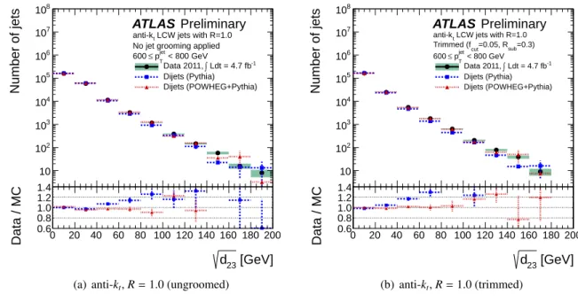
Splitting scales:

The k

t

splitting scales are defined by reclustering the constituents of a jet with the k

t

recombination algorithm. The k

_t

-distance of the final step in combining two proto-jets, referred to as subjets in this case, into the final jet can be used to define a “splitting scale” variable given in Eq. (5) as:

q

d

i j=

min(p

Ti,

p

_Tj

)

×∆

R

i j ,

(5) where

∆

R

i j

is the distance between the two subjets. With this definition, the subjets identified at the last step of the reclustering in the k

_t

algorithm provide the

√

d

₁₂

observable. Similarly,

√

d

₂₃

defines the splitting scale in the second to the last step of the reclustering. These definitions are equivalent to the square root of the distance parameter

ρi j

given in Eq. (2) multiplied by the jet radius parameter R in order to remove the explicit dependence on the nominal jet radius. As described in Section

2.2, the

k

t

algorithm combines the harder constituents last. Because of this, and the fact that

p

d

i j

uses the minimum p

_T

between the i and j subjets, the parameters

√

d

₁₂

and

√

d

₂₃

can be used to distinguish heavy particle decays, which tend to be reasonably symmetric, from largely asymmetric splittings in light quark or gluon jets. The expected value for a two-body heavy particle decay is approximately

√

d

₁₂≈

m

^jet/2, whereas jets from the parton shower of light

quarks and gluons will tend to exhibit a steeply falling spectrum for both

√

d

₁₂

and

√

d

₂₃

(see Figure

23

in Section

5.3).

N-subjettiness:

The N-subjettiness variables

τN

[14,

15] are observables related to the subjet multiplic-

ity. The

τN

variable is calculated by clustering the constituents of the jet with the k

t

algorithm and requiring exactly N subjets to be found. This is done using the exclusive k

t

algorithm [11]

and is based on reconstructing clusters of particles in the jet using all of the jet constituents. The exclusive mode of the k

t

algorithm discards constituents for which

ρiB < ρi j

and stops clustering either when all

ρiB

and

ρi j

are above some specified

ρ_cut

or when there are N proto-jets remaining.

The latter case is used here. These N final subjets define axes within the jet, around which the jet constituents may be concentrated. The variables

τN

are then defined in Eq. (6) as the sum over all constituents k of the jet:

τN =

1

d

₀ X

k

p

_Tk×

min(δR

_1k, δR_2k, ..., δRNk

) , with d

₀≡X

k

p

_Tk×

R (6)

where R is the jet radius parameter in the jet algorithm, p

_Tk

is the p

_T

of constituent k and

δRik

is the distance from the subjet i to constituent k. Using this definition,

τN

describes how well jets can be described as containing N or fewer k

_t

subjets by assessing the degree to which constituents are localized near the axes of these subjets. The ratios

τ₂/τ₁

and

τ₃/τ₂

can be used to provide discrim- ination between jets formed from the parton shower of light quarks or gluons and jets containing two hadronic decay products (from Z-bosons, for example) or three hadronic decay products from boosted top quarks. These ratios will herein be referred to as

τ₂₁

and

τ₃₂

respectively. For example,

τ₂₁ '

1 corresponds to a jet that is very well described by a single subjet whereas a lower value implies a jet that is much better described by two subjets than one.

2.4 Jet grooming algorithms

Mass-drop Filtering:

The mass-drop filtering procedure seeks to isolate concentrations of energy within a jet by identifying relatively symmetric subjets, each with a significantly smaller mass than that of their sum. This technique was developed and optimized using C/A jets in the search for a Higgs boson decaying to two b-quarks: H

→

b b ¯ [16]. The procedure is applied only to C/A jets since each clustering step of the algorithm combines the two widest angle proto-jets at that point in the shower history. Therefore, the structure of the C/A jet provides an angular-ordered description of substructure, which tends to be one of the most useful properties when searching for hard splittings within a jet. Although the mass-drop criterion and subsequent filtering procedure are not specifi- cally based on soft-p

_T

or wide-angle selections, the algorithm does retain the hard components of the jet through the requirements placed on its internal structure. The first measurements of the jet mass of these filtered jets was performed using 35 pb

⁻¹

of data collected in 2010 by the ATLAS experiment [17].

The mass-drop

/

filtering procedure has two stages:

• Mass-drop and symmetry

Undo the last stage of the C/A clustering so that the jet “splits”

into two subjets, j

₁

and j

₂

, ordered such that the mass of j

₁

is larger: m

^j1 >

m

^j2

. The mass- drop criterion requires that there be a significant di

ff

erence between the original jet mass (m

^jet

) and m

^j1

after the splitting:

m

^j1/m^jet< µ_frac,

(7)

5

where

µ_frac

is a parameter of the algorithm. The splitting is also required to be relatively symmetric:

min[( p

_T^j1

)

²,

( p

_T^j2

)

²

] (m

^jet

)

² ×∆

R

²_j

1,j₂ > y_cut,

(8)

where

∆

R

_j1,j2

is the opening angle between j

₂

and j

₁

, and

y_cut

defines the energy sharing between the two highest p

_T

subjets within the original jet. For the analyses presented here,

y_cut

is set to 0.09, the optimal value obtained in previous studies [16]. To give a sense of the kinematic requirements that this places on a given decay, consider a hadronically decaying W boson with p

^W_T ≈

200 GeV. According to the approximation given by Eq. (1), the average angular separation of the two daughter quarks is

∆

R

j₁,j₂ ∼

0.8. The symmetry requirement determined by

ycut

in Eq. (8) thereby implies that the transverse momentum of the softer (in p

_T

) of the two subjets be greater than approximately 30 GeV. Generally, the requirement entails a minimum p

_T

of the softer subjet of p

^subjet_T /

p

^jet_T >

0.15, thus forcing both subjets to carry some significant fraction of the momentum of the original jet. This procedure is illustrated in Figure

2(a). If the mass-drop and symmetry criteria are not satisfied, the jet is

discarded.

• Filtering

The constituents of j

₁

and j

₂

are reclustered using the C/A algorithm with R

_filt <

∆

R

j₁,j₂

, where R

_filt =

min[0.3,

^∆R₂^j1,j2

]. The jet is then filtered; all constituents outside the three hardest subjets are discarded. In isolating j

₁

and j

₂

with the C/A algorithm, the angular scale of any potential massive particle decay is known. By dynamically reclustering the jet at an appropriate angular scale able to resolve that structure, the sensitivity to highly collimated decays is maximized. This is illustrated in Figure

2(b).

In this analysis, three values of the mass-drop parameter

µ_frac

are studied, as summarized in Table

1. The values chosen for µ_frac

are based on a previous study [16] which has shown that

µ_frac=

0.67 is optimal in discriminating H

→

b b ¯ from background. A subsequent study regarding the factorization properties of several groomed jet algorithms [18] found that smaller values of

µ_frac

(0.20 and 0.33) are similarly e

ff

ective at reducing backgrounds, and yet they remain factoris- able within the soft collinear effective theory studied in that analysis. Future studies may seek to evaluate the impact of variations of

y_cut

as well as

µ_frac

, in particular to assess the extent to which mass-drop filtering may be used for three-body decays, for example from the top quark.

Trimming:

The trimming algorithm [19] takes advantage of the fact that contamination from pile-up, multiple parton interactions (MPI), and initial-state radiation (ISR) in the reconstructed jet is often much softer than the outgoing partons associated with the hard-scatter and their final-state radiation (FSR). The ratio of the p

_T

of the constituents to that of the jet is used as a selection criterion. Com- pletely removing the softer components from the final jet is possible as there is generally minimal spatial overlap of the soft additional radiation from pile-up, MPI, and ISR with the hard-scatter decay products. As the primary effect of pile-up, for example, is additional low-energy topo-clust- ers as opposed to additional energy being added to topo-clusters from hard-scatter particles, this allows a relatively simple jet energy o

ff

set correction for smaller radius jets (R

=

0.4, 0.6) as a function of the number of primary reconstructed vertices [5].

The trimming procedure uses a k

_t

algorithm to create subjets of size R

_sub

from the constituents

of a jet. Any subjets with p

T i/

p

^jet_T <

f

_cut

are removed, where p

T i

is the transverse momentum

of the i

^th

subjet, and f

_cut

is a parameter of the method, which is typically a few percent. The

remaining constituents form the trimmed jet. This procedure is illustrated in Figure

3. Low-mass

jets (with m

^jet<

100 GeV) from a light quark or gluon typically lose 30-50% of their mass, while

jets containing the decay products of a boosted object will lose only a few percent of their mass,

(a) The mass drop and symmetric splitting criteria.

(b) Filtering.

Figure 2: A cartoon depicting the two stages of the mass-drop filtering procedure.

Figure 3: A cartoon depicting the jet trimming procedure.

most of which is due to the removal pileup or the UE (see, for example, Figures

22

and

25

in Section

5.3). The fraction removed increases with the number of interactions in the event [1].

Six configurations of trimmed jets are studied here, arising from combinations of f

_cut

and R

_sub

, given in Table

1. They are based on the optimized parameters in Ref. [19] (

f

_cut=

0.03, R

_sub=

0.2) and variations suggested by the authors of the algorithm. This set represents a wide range of phase space for trimming and is somewhat broader than considered in the original paper on the subject.

7

Pruning:

The pruning algorithm [20,

21] is similar to trimming in that it removes constituents with a

small relative p

_T

, but additionally utilizes a wide-angle radiation veto. The pruning procedure is invoked at each successive recombination of the jet algorithm used (either C/A or k

t

), based on the branching at each point in the jet reconstruction, and as such does not require the reconstruction of subjets. This results in definitions of the terms “wide-angle” or “soft” that are not directly related to the original jet but rather to the proto-jets formed in the process of rebuilding the pruned jet.

Figure 4: A cartoon illustrating the pruning procedure.

The procedure is as follows:

•

Run either the C/A or k

_t

recombination jet algorithm on the constituents found by any jet finding algorithm.

•

At each recombination step with constituents j

₁

and j

₂

(where p

_T^j1 >

p

_T^j2

), require that p

_T^j2/p_T^j1+j2>

z

_cut

or

∆

R

j₁,j₂ <

R

_cut× ^2mjet

p^jet

T

.

•

Merge j

₂

with j

₁

if the above criteria are met, otherwise, discard j

₂

and continue with the algorithm.

The pruning procedure is illustrated in Figure

4. Six configurations, given in Table 1, based on

combinations of z

_cut

and R

_cut

are studied here. They are not configurations that have been stud- ied before in Refs. [20,

21] but are chosen based on discussion with the authors of the pruning

algorithm [22]. This set of parameters also represents a relatively wide range of possible configu- rations.

2.5 HEPTopTagger

The HEPTopTagger [23] is an example of how jet grooming techniques may be used to optimize the selection of boosted objects (in this case, top quarks with a hadronically-decaying W boson daughter) over a large multi-jet background. The method uses the C/A jet algorithm and a variant on the mass- drop filtering technique described in Section

2.4

in order to utilize information about the recombination history of the jet. The algorithm proceeds as follows:

• Decomposition into substructure objects:

The mass-drop criterion defined in Eq. (7) is applied

to a large-R C

/

A jet, where j

₁

and j

₂

are the two subjets from the last stage of clustering. If the

criterion is satisfied, the same prescription is followed iteratively on both j

₁

and j

₂

until N

i

subjets

are left, where the subjets either have masses m

_i ≤

m

_cut

or represent individual constituents, such

Jet finding algorithms used Grooming algorithm Configurations considered C/A Mass-Drop Filtering

µ_frac=

0.20, 0.33,

0.67

anti-k

t

and C/A Trimming f

_cut=

0.01,

0.03, 0.05

R

_sub=0.2, 0.3

anti-k

t

and C/A Pruning R

_cut=

0.1, 0.2, 0.3

z

_cut=

0.05, 0.1

C/A HEPTopTagger (see Table

2)

Table 1: Summary of the grooming configurations considered in this study. Values in boldface are optimized configurations reported in Ref. [16] and Ref. [19] for filtering and trimming, respectively.

as topo-clusters, tracks, or truth particles (i.e. no clustering history). If at any stage m

^j1 >

m

^jetµ_frac

, the mass-drop criterion and subsequent iterative de-clustering is not applied to j

₂

. The values of m

_cut

and R studied in this note are summarized in Table

2.

R values of 1.5 and 1.8, somewhat larger than used generally in mass-drop filtering, are chosen based on previous studies [23]. When the iterative process of de-clustering the jet is complete, there must exist at least three substructure objects, otherwise the jet is discarded.

• Filtering:

Combinations of three substructure objects are filtered at a time. The constituents of the substructure objects in a given triplet are reclustered into N

_i

subjets using the C/A algorithm with a distance parameter R

_filt=

min[0.3,

^∆R₂^j1,j2

], where

∆

R

j₁,j2

is the minimum separation between all possible pairs in the current triplet.

• Top mass window requirement:

If the invariant mass of the four-vector determined by summing the constituents of the N

i

subjets is not in the range 140

≤

m

^jet <

200 GeV then the triplet combination is ignored. If more than one triplet satisfies the criteria, only the one with mass closest to the top quark mass, m

_top

, is used.

• Reclustering of subjets:

From the N

i

subjets formed from the chosen top candidate triplet, a number of leading-p

_T

subjets (N

_subjet

) are chosen, where 3

≤

N

_subjet≤

N

_i

. Of these chosen subjets, exactly three jets are built by applying the C

/

A algorithm to the constituents of the N

_subjet

subjets (exclusive clustering using a distance parameter R

jet

listed in Table

2). These subjets are calibrated

as described in [24].

•

W

boson mass requirements:

Relations listed in A1 of [23] are defined using the total invariant mass of the three subjets (m

123

) and the invariant mass m

i j

formed from combinations of two of the three C/A jets ordered in p

_T

. These relations include:

R

−<

m

₂₃

m

₁₂₃ <

R

₊

(9)

0.2

<

arctan m

₁₃

m

₁₂ <

1.3 (10)

Here, R

_± =

(1

±

f

_W

)

_m^mW

top

, f

_W

is a resolution variable (given in Table

2), and the quantities

m

_W

and m

_top

denote the W boson and top quark masses, respectively. If at least one of the criteria in A1 of [23] is met, the four-momentum addition of the three subjets is considered a candidate top quark.

9

The procedure is illustrated in Figure

5.

Default Tight Loose Large

R 1.5 1.5 1.5 1.8

m

_cut

[GeV] 30 30 70 30

R

_jet

0.3 0.2 0.5 0.3

N

_s

5 4 7 5

f

W

[%] 15 10 20 15

Table 2: The settings used for studying the performance of the HEPTopTagger.

(a) Every object encountered in the de-clustering process is considered a

‘substructure object’ if it is of sufficiently low mass or has no clustering history.

(b) The mass-drop criterion is applied iteratively, following the highest subjet-mass line through the clustering history, resulting inNisubstructure objects.

(c) For every triplet-wise combination of the substructure objects, recluster into subjets and select theNsubjetleading-pTsubjets, with 3≤Nsubjet≤Ni(here,Nsubjet=5).

(d) Recluster the constituents of theNsubjet subjets into exactly three subjets to make the top candidate for this triplet-wise combination of substructure ob- jects.

Figure 5: The HEPTopTagger procedure.

11

3 Data and Monte Carlo Samples

3.1 Data quality criteria and event selection

The data used in the analyses presented in this note, corresponding to (4.7

±

0.2) fb

⁻¹

of integrated luminosity, are required to have met baseline quality criteria and were taken during periods in which the detector was fully operational. The ATLAS data quality (DQ) criteria reject data with significant contamination from detector noise or issues in the read-out based upon individual assessments for each subdetector. These criteria are established separately for the barrel, endcap and forward regions, and differ depending on the trigger conditions and reconstruction of each type of physics object, such as jets, electrons, muons, etc. The primary systems of interest in these studies are the electromagnetic and hadronic calorimeters and the inner tracking detector (the latter specifically for studies of the properties of tracks associated with jets).

To reject non-collision backgrounds, events are required to contain a primary vertex consistent with the LHC beam spot, reconstructed from at least 2 tracks each with transverse momentum p

^track_T >

400 MeV. All jets in the event reconstructed with the anti-k

t

algorithm with R

=

0.4 and a measured p

^jet_T >

20 GeV are required to satisfy the “looser” requirements discussed in detail in Ref. [25]. These selections are designed to provide an e

ffi

ciency to retain good quality jets of greater than 99.8% with as high a fake jet rejection as possible. In particular, this selection is very efficient at rejecting fake jets that arise due to calorimeter noise.

A three-level trigger system is used to select interesting events. The level-1 trigger is implemented in hardware and uses a subset of detector information to reduce the event rate to a design value of at most 75 kHz. This is followed by two software-based triggers, level-2 and the event filter, which together reduce the event rate to a few hundred Hz. Events used in this analysis were selected if the leading jet in the event passed a single jet trigger at the event filter stage with p

^jet_T >

350 GeV. This trigger threshold was un-prescaled for the entire 2011 data-taking period and thus represents the full integrated luminosity with negligible ine

ffi

ciency.

3.2 Monte Carlo simulation

The data are compared to inclusive jet events generated by two MC simulations: PYTHIA 6.425 [2] and POWHEG-BOX 1.0 [3,4,26] (patch 4) interfaced to PYTHIA 6.425 for the parton shower, hadronization, and underlying event (UE) models. In the former case, standalone PYTHIA uses the modified-LO parton distribution function (PDF) set MRST LO* [27]. In the latter, POWHEG

+

PYTHIA uses the CTEQ6L1 PDF set [28]. For both cases, PYTHIA is tuned with the corresponding AUET2B tune [29,

30]. The

comparison between PYTHIA and POWHEG

+

PYTHIA represents an important juxtaposition, at least at the matrix element (ME) level, between an LO (PYTHIA) and an NLO (POWHEG) ME generator.

After simulation of the parton shower and hadronization, events are passed through the full Geant4 [31]

detector simulation [32]. Following this, the same trigger, event, quality, jet, and track selection criteria are applied to the MC simulation as are applied to the data.

Several samples of events containing boosted hadronic particle decays are used for direct compar- isons of the performance of the various reconstruction and jet substructure techniques. For two-prong decays, a sample of hadronically decaying Z bosons was generated using the HERWIG 6.5.10 [33] event generator interfaced with JIMMY 4.3.1 [34] for MPI. In order to test the performance of techniques de- signed for three-prong decays, t¯ t events from an additional heavy gauge boson (Z

⁰

with m

_Z⁰ =

1.6 TeV) were generated using the same PYTHIA 6.425 tune as stated above. This model provides a relatively narrow t¯ t resonance and very high p

_T

top quarks.

Pile-up is simulated by overlaying additional soft pp collisions, or minimum bias events, which are

generated with PYTHIA 6.425 using the ATLAS MC11 AUET2B tune [30] and the CTEQ6L1 PDF

set. The minimum bias events are overlaid onto the hard scattering events according to the measured distribution of the average number

hµi

of pp interactions per bunch crossing. The proton bunches were organized in four trains of 36 bunches with a 50 ns spacing between the bunches. Therefore, the simu- lation also contains effects from out-of-time pile-up, i.e. contributions from the collision of neighboring bunches to that where the event of interest occurred. Simulated events are reweighted such that the MC distribution of

hµi

agrees with the data, as measured by the luminosity detectors in ATLAS [35].

4 Calibration of Large-R and Groomed Jets

This section describes the procedure used for determining the energy and mass scale calibrations for large-R and groomed jets using Monte Carlo simulation. In addition, the impact of detector simulation and the partonic origin of a jet on the mass calibration and response are studied.

4.1 Monte Carlo based calibration

The MC calibration scheme starts from the measured calorimeter energy at the electromagnetic (EM) en- ergy scale [36–44], which correctly measures the energy deposited by electromagnetic showers. A local cluster weighting (LCW) calibration method first clusters together topologically connected calorime- ter cells and classifies these clusters as either electromagnetic or hadronic. Based on this classification energy corrections are derived from single pion MC simulations. Dedicated hadronic corrections are derived for the effects of non-compensation, signal losses due to noise suppression threshold effects, and energy lost in non-instrumented regions. The results shown here use LCW clusters as input to the jet algorithm.

The final jet energy calibration is derived as a correction relating the calorimeter’s response to the true jet energy. It can be applied to EM scale jets, with the resulting calibrated jets referred to as EM

+

JES, or to LCW calibrated jets, with the resulting jets referred to as LCW+JES jets. More details regarding the evaluation and validation of this approach for standard anti-k

t

R

=

0.4, 0.6 jets can be found in Ref. [5].

The JES correction is derived from a PYTHIA MC sample including pile-up events, as in the standard JES determination procedure [5]. For standard jet algorithms, the dependence of the jet response on the number of primary vertices (N

PV

) and the average number of interactions (< µ >) is removed by applying a pile-up o

ff

set correction on the EM or LCW scale before applying the JES correction. However, for large-R jets and jets with the various grooming algorithms applied, no explicit pile-up correction is applied.

4.2 Jet mass scale determination

Since one of the primary goals of the use of large-R and groomed jet algorithms is to reconstruct the masses of jets accurately and precisely, a last step is added to the calibration procedure of large-R jets wherein the mass of the jet is calibrated based on multi-jets MC simulation. Explicit jet mass calibration is important for using the individual invariant jet mass in physics analyses since it is particularly suscep- tible to soft, wide-angle contributions that do not otherwise significantly impact the jet energy scale. The procedure measures the jet mass response for jets built from LCW clusters after the standard JES cali- bration. The mass response is determined from the mean of a Gaussian fit to the core of the distribution of the reconstructed jet mass divided by the corresponding truth jet mass.

Figure

6

shows the jet mass response in a number of jet energy bins as a function of

η, before and

after calibration to the true jet mass for anti-k

t

, R

=

1.0 jets. One can see from this figure that even very high p

_T

jets near the central part of the detector can have a mean mass scale (or JMS) up to 20% di

ff

erent than that of the particle level true jet mass. In particular, the reconstructed mass is, on average, greater

13

than that of the particle-level jet due in part to noise and pile-up in the detectors. Additionally, the finite resolution of the detector has a di

ff

erential impact on the mass response as a function of

η. Following the

jet mass calibration, performed also as function of

η, a uniform mass response can be restored to within

3% across the full energy and

η

range.

4.3 In-situ validation based on track jets

In order to validate the jet mass measurement made by the calorimeter, calorimeter-based jets are com- pared to track jets reconstructed from charged particle tracks. Track jets have a very di

ff

erent set of systematic uncertainties and allow for a reliable determination of the relative systematic uncertainties associated with the calorimeter-based measurement. Performance studies [45] have shown that there is excellent agreement between the measured positions of clusters and tracks in data, indicating no system- atic misalignment between the calorimeter and the inner detector.

The use of track jets reduces or eliminates the impact of additional pp collisions by requiring the jet inputs (tracks) to come from the hard-scattering vertex. It also provides a reference with which to compare the calorimeter jet measurement. The inner detector and calorimeter have largely uncorrelated systematic e

ff

ects, and so comparison of variables such as jet mass and energy between the two systems allows for a separation of physics and detector e

ff

ects. It is therefore possible to validate the JES and JMS and also to estimate the pile-up energy contribution to jets directly. This approach was used extensively in the measurement of the jet mass and substructure properties of jets in the 2010 data [17] where pile-up was significantly less important and the statistical reach of the measurement was smaller than with the full integrated luminosity of 4.7 fb

⁻¹

for the 2011 dataset.

The method to determine the relative uncertainty uses the ratio of the calorimeter p

^jet_T

(m

^jet

) to the track jet transverse momentum, p

^{track jet}_T

(m

^{track jet}

). The ratios are defined explicitly as

r

_{track jet}^pT =

p

^jet_T

p

^{track jet}_T

,

r

_{track jet}^m =

m

^jet

m

^{track jet},

(11)

where the matching between calorimeter and track jets is performed using a matching radius of

∆

R

<

0.3.

These ratios are expected to be well described by the detector simulation in the case that detector e

ff

ects are well modeled. That is to say, even if some underlying physics process was unaccounted for by the simulation, as long as this process a

ff

ects both the track jet and calorimeter jet p

_T

or masses in a similar way, then the ratio of data to simulation should be relatively una

ff

ected.

Double ratios of r

_{track jet}^m

and r

_{track jet}^pT

are constructed in order to evaluate this agreement. These double ratios, R

_r^pT_{track jet}

and R

^m_{rtrack jet}

, are defined as:

R

_r^pT_{track jet} =

r

_{track jet}^pT,data

r

_{track jet}^pT,MC

,

R

^m_{rtrack jet} =

r

^m,data_{track jet}

r

^m,MC_{track jet}.

(12)

The dependence of R

_r^pT_{track jet}

and R

^m_{rtrack jet}

on p

^jet_T

and m

^jet

provides a test for the deviation between data and simulation, thus allowing for an estimation of the calibration uncertainty.

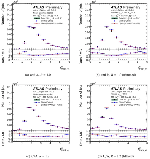
Figure

7

shows the distribution of r

_{track jet}^m

for four jet algorithms and trimming configurations, and for

jets in the range 500

≤

p

^jet_T <

600 GeV in the central calorimeter region,

|η|<

0.8. This p

^jet_T

range is fairly

typical and was chosen for illustrative purposes because of its relevance to boosted vector bosons and

boosted tops, as the decay products of both are expected to be fully merged into a large-R jet. The peak

position near r

_{track jet}^m ≈

2 and the shape of the distribution are both generally well-described. Both the

ungroomed and the trimmed anti-k

t

, R

=

1.0 distributions show some discrepancies at very low r

^m_{track jet}

,

η Jet -5 -4 -3 -2 -1 0 1 2 3 4 5

Jet mass response before calibration

0 0.5 1 1.5 2 2.5 3 3.5 4

E = 50 GeV E = 100 GeV E = 250 GeV

E = 500 GeV E = 750 GeV E = 1500 GeV

ATLAS Preliminary - Simulation

LCW jets with R=1.0, No grooming applied anti-kt

Dijets (Pythia) Before mass calibration

(a) anti-kt,R=1.0, before calibration

η Jet -5 -4 -3 -2 -1 0 1 2 3 4 5

Jet mass response after calibration

0 0.5 1 1.5 2 2.5 3 3.5 4

ATLAS Preliminary - Simulation

LCW jets with R=1.0, No grooming applied anti-kt

Dijets (Pythia) After mass calibration

η Jet -1.5 -1-0.5 0 0.5 1 1.5

Response

0.95 1 1.05

(b) anti-kt,R=1.0, after calibration

Figure 6: Mass response

(a)

before and

(b)

after mass calibration for ungroomed anti-k

t

, R

=

1.0 jets.

The dotted line shown in

(b)

represents a

±3% envelope on the precision of the final jet mass scale

calibration.

where the description of very soft radiation and hadronization is important, and at high values of r

^m_{track jet}

, above r

^m_{track jet} &

4. The differences are of order 20%. However, these spectra are used primarily to test the overall scale, so that the important comparison is of the mean value of the distributions. These are quite well described, as discussed in Section

4.4.

4.4 Evaluation of jet mass scale systematics

The relative systematic uncertainty on the jet kinematics is first estimated for each MC generator sample as the weighted average absolute deviation of the double ratio, R

^m_{rtrack jet}

, from unity. Measurements of R

^m_{rtrack jet}

are performed in exclusive p

^jet_T

and

η

ranges. The statistical uncertainty is used as the weight in this case. The final relative uncertainty is then determined by the maximum of the weighted average relative uncertainties considered. Comparisons are made using PYTHIA and POWHEG

+

PYTHIA.

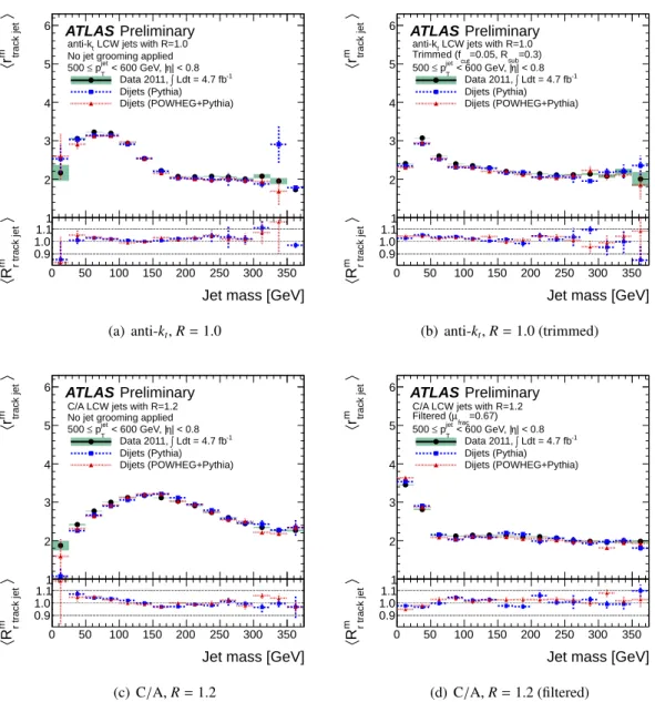
Figure

8

presents the distributions of both r

^m_{track jet}

and the double ratio with respect to MC, R

^m_{rtrack jet}

, for the same four jet algorithms and grooming configurations as shown in Figure

7. In the peak of the jet

mass distribution, logarithmic soft terms dominate [46] and lower p

_T

particles constitute a large fraction of the calorimeter jet mass. These particles are often bent by the magnetic field or not reconstructed as charged tracks and thus contribute less to the track jet mass, resulting in the shape observed in the r

^m_{track jet}

distribution in this region. Higher mass jets tend to be composed of higher p

_T

particles that contribute more similarly to the calorimeter and track-based mass reconstruction, resulting in a flatter and fairly stable r

^m_{track jet}

ratio. This flat r

^m_{track jet}

distribution is present across the mass range for both filtered and trimmed jet masses, as both these algorithms are designed to remove softer particles as compared to the original jet p

_T

. Although there is a di

ff

erence in the phase space of emissions probed at low mass and high mass, the calorimeter response relative to the tracker response is well modeled by both PYTHIA and POWHEG MCs.

The weighted average deviation of R

^m_{rtrack jet}

from unity ranges from approximately 2% to 4% for the set of jet algorithms and grooming configurations tested for jets in the range 500

≤

p

^jet_T <

600 GeV and in the central calorimeter,

|η| <

0.8. The results are fairly stable for the slightly less central

η

range

15

Number of jets

0.02 0.04 0.06 0.08 0.1 0.12 0.14 0.16 0.18

106

×

track jet

rm

0 1 2 3 4 5 6

Data / MC

0.6 0.8 1.0 1.2 1.4

ATLAS Preliminary

LCW jets with R=1.0 anti-kt

No jet grooming applied

| < 0.8 η < 600 GeV, | T pjet

≤ 500

Ldt = 4.7 fb-1

∫ Data 2011, Dijets (Pythia) Dijets (POWHEG+Pythia)

(a) anti-kt,R=1.0

Number of jets

0.02 0.04 0.06 0.08 0.1 0.12 0.14 0.16

106

×

track jet

rm

0 1 2 3 4 5 6

Data / MC

0.6 0.8 1.0 1.2 1.4

ATLAS Preliminary

LCW jets with R=1.0 anti-kt

=0.3)

=0.05, Rsub cut Trimmed (f

| < 0.8 η < 600 GeV, | T pjet

≤ 500

Ldt = 4.7 fb-1

∫ Data 2011, Dijets (Pythia) Dijets (POWHEG+Pythia)

(b) anti-kt,R=1.0 (trimmed)

Number of jets

0.02 0.04 0.06 0.08 0.1 0.12 0.14 0.16

106

×

track jet

rm

0 1 2 3 4 5 6

Data / MC

0.6 0.8 1.0 1.2 1.4

ATLAS Preliminary

C/A LCW jets with R=1.2 No jet grooming applied

| < 0.8 η < 600 GeV, | T pjet

≤ 500

Ldt = 4.7 fb-1

∫ Data 2011, Dijets (Pythia) Dijets (POWHEG+Pythia)

(c) C/A,R=1.2

Number of jets

10 20 30 40 50 60 70 80

103

×

track jet

rm

0 1 2 3 4 5 6

Data / MC

0.6 0.8 1.0 1.2 1.4

ATLAS Preliminary

C/A LCW jets with R=1.2

=0.67) µfrac Filtered (

| < 0.8 η < 600 GeV, | T pjet

≤ 500

Ldt = 4.7 fb-1

∫ Data 2011, Dijets (Pythia) Dijets (POWHEG+Pythia)

(d) C/A,R=1.2 (filtered)

Figure 7: r

^m_{track jet}

distributions for

(a)

anti-k

t

, R

=

1.0,

(b)

anti-k

t

, R

=

1.0 trimmed jets ( f

_cut =

0.05, R

_sub =

0.03),

(c)

C/A, R

=

1.2 jets, and

(d)

C/A, R

=

1.2 filtered jets (µ

_frac =

0.67) in the

range 500

≤

p

^jet_T <

600 GeV and in the central calorimeter,

|η| <

0.8. The ratios between data and MC

distributions are shown in the lower section of each figure.

0.8

≤ |η|<

1.2.

Figure

9

presents the full set of jet mass scale systematic uncertainties for various jet algorithms estimated using the calorimeter-to-track jet double ratios. The total relative uncertainty includes the 3%

uncertainty of the precision of the jet mass scale calibration (see

6(b), for example) as well as the uncer-

tainty on the track measurements themselves. The latter uncertainty takes into account the knowledge of tracking inefficiencies and their impact on the p

^jet_T

and m

^jet

measurements using track jets. Each of these two additional components is assumed to be uncorrelated and added in quadrature with the uncertainty determined solely from the calorimeter-to-track jet double ratios.

The impact of the tracking efficiency systematic uncertainty on r

^m_{track jet}

is evaluated by randomly rejecting tracks used to construct track jets according to the efficiency uncertainty. This is evaluated as a function of

η

and m

^jet

for various p

^jet_T

ranges. Typically, this results in a 2-3% shift in the measured track jet kinematics (both p

_T

and mass) and thus a roughly 1% shift on the resulting total uncertainty.

The total systematic uncertainty on the jet mass scale is fairly stable near 4–5% for all jet algorithms up to p

^jet_T ≈

800 GeV. At low p

^jet_T

, in the range 200

≤

p

^jet_T <

300 GeV, the average uncertainty for some jet algorithms rises to approximately 5–7%. The estimated uncertainty is similar for both the ungroomed and the trimmed or filtered jets, except for trimmed anti-k

t

jets (see Figure

9(b)) for which the uncertainty

in the range 900

≤

p

^jet_T <

1000 GeV is approximately 8%.

17