Reconstruction and Modelling of Jet Pull with the ATLAS Detector

(1)

ATLAS-CONF-2014-048 11/07/2014

ATLAS NOTE

ATLAS-CONF-2014-048

July 10, 2014

Minor revision: July 11, 2014

Reconstruction and Modelling of Jet Pull with the ATLAS Detector

The ATLAS Collaboration

Abstract

Weighted radial moments over the constituents of a jet have previously been shown to be an experimental handle on colour connections between the initiating partons. This note presents a study of the detector performance in reconstructing one such moment, the jet pull angle for jets produced in t¯ t events with one leptonically decaying W boson using 20.3 fb

⁻¹

of data recorded with the ATLAS detector at

√

s

=

8 TeV.

Revised labels on figures 15-17 and references with respect to the version of July 10, 2014

c

Reproduction of this article or parts of it is allowed as specified in the CC-BY-3.0 license.

(2)

1 Introduction

Due to the confining nature of the strong force, probing the chromodynamic connections between partons produced in pp collisions at the Large Hadron Collider (LHC) directly is not possible. However, some information from the colour connections of partons is retained by the observable objects - collimated streams of particles known as jets. First defined in Ref. [1], the jet pull is a kinematic variable built from momentum-weighted radial moments of jet constituents (jet substructure) combined with information from the relative orientations of jets in the event (jet superstructure) that was designed to be sensitive to the colour flow between the initiating partons of jets. Probing colour flow with the ATLAS detector is interesting in its own right as a direct probe of quantum chromodynamics, and can also be used as a discriminating variable to isolate colour singlets such as Higgs bosons from colour octets (e.g. gluons) as suggested in Ref. [2] and used experimentally in Ref. [3–5]. The first experimental study of colour connection using jet pull was performed on another colour singlet, the W boson, at D0 [6]. The purpose of this note is to establish the detector performance aspects of jet pull, so that it can be used in future physics measurements with ATLAS. Section 2 formally defines the jet pull angle and sets the notation and nomenclature. Section 3 describes the object and event selection. Section 4 contains the main results of the note, describing the impact of the detector response on the jet pull angle distribution. There are separate subsections describing the reconstructed jet pull angle distribution (4.1), the inclusive detector response (4.2) as well as the dependence of the response on kinematics (4.3), the dependence of the response on the distribution of constituents (4.4), and relationships between the jet pull angle (response) and other event properties (4.5). Finally, Section 5 shows the distribution of the jet pull angle in the data and compares with the simulation as a validation of the features observed in the reconstructed simulation in Section 4.

2 Jet Pull

The pull vector for a jet J is

vP

( J)

= P

i∈J pⁱ_T|~r_i|

p^J_T ~

r

_i

, where the sum runs over constituents of the jet J and

~

r

_i =

(

∆yi,∆φi

) with respect to the position of the jet axis in rapidity (y) - azimuthal angle (φ) space

¹

. Given the pull vector for jet J

₁

, a variable sensitive to the underlying colour connections to another jet J

₂

is the angle the pull vector for J

₁

makes with respect to the vector connecting J

₁

and J

₂

in (∆

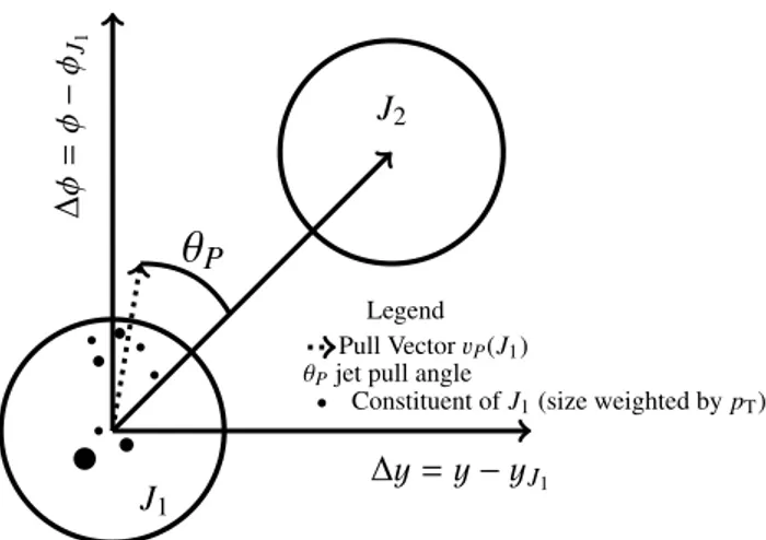
y,∆φ) [1].

This jet pull angle is shown graphically in Fig. 1 and will be denoted

θP

( J

₁,

J

₂

). For physics processes that preserve Lorentz symmetry, only the magnitude of

θP

(for

−π < θP ≤ π) is relevant and so henceforth, θP

(J

1,

J

₂

) refers to modulus of the angle in (∆

y,∆φ) space. Since the pull vector is weighted by

p

_T

and

∆

R

= p

∆η²+ ∆φ²

to the jet axis, large angle soft radiation can be important. The magnitude of the pull vector,

|vP

(J)

|

, will be discussed in the context of the pull angle resolution in Sec. 4.4.

1ATLAS uses a right-handed coordinate system with its origin at the nominal interaction point (IP) in the centre of the detector and thez-axis along the beam pipe. Thex-axis points from the IP to the centre of the LHC ring, and they-axis points upward. Cylindrical coordinates (r, φ) are used in the transverse plane,φbeing the azimuthal angle around the beam pipe. The pseudorapidity is defined in terms of the polar angleθasη=−ln tan(θ/2). Transverse momentum and energy are defined in the x−y-plane aspT=p·sin(θ) andET =E·sin(θ).

1

(3)

∆y=y−yJ₁

∆φ=φ−φJ1

J

₂

Legend Pull Vectorv_P(J1) θPjet pull angle

Constituent ofJ₁(size weighted byp_T)

J

₁

θ

_P

Figure 1: A schematic diagram depicting the construction of the jet pull angle between jets J

₁

and J

₂

.

3 Object and Event Selection

ATLAS is a multipurpose particle detector at the LHC comprising four main subsystems: an inner track- ing detector (ID), electromagnetic and hadronic calorimeters, and a muon spectrometer. It has an ap- proximately cylindrical geometry with close to 4π solid angle coverage, and tracking in the ID extending to pseudorapidity

|η|<

2.5. For an in-depth description of the detector, see Ref. [7].

In order to investigate detector performance aspects of the jet pull angle, several jet definitions are employed. Reconstructed jets are clustered with the anti-k

t

algorithm [8] with radius parameter 0.4 from topological calorimeter clusters [9], treated as massless. Clusters are calibrated using the local cluster weighting (LCW) algorithm [10], and jets are calibrated to account for a reconstruction bias as well as to mitigate the contribution from pileup [11]. To investigate jet pull angle properties in simulation without the distortions arising from detector resolution, truth jets are formed from the four-vectors of Monte Carlo (MC) stable particles

²

(excluding

µ

and

ν) as inputs to the anti-kt

R

=

0.4 clustering algorithm.

The jet pull vector is a weighted sum over jet constituents. Studies in this note exploit di

ff

erent sets of jet constituents: for reconstructed jets, the nominal constituents are the calorimeter clusters used in the jet construction (calorimeter pull). Truth jets correspondingly use all MC stable particles (all particles pull). Alternatively, the tracks assigned to a jet can be used as constituents in the pull vector calculation (track pull). These tracks

³

are required to have p

_T ≥

500 MeV,

|η| <

2.5, and a

χ²

per degree of freedom (resulting from the track fit) less than 3.0. Additional quality criteria are applied to select tracks originating from the collision vertex [12]. Tracks are associated to jets using ghost-association [13]: an assignment of tracks to jets by adding to the jet clustering process ghost versions of tracks that have the same direction but infinitesimally low p

_T

. The corresponding constituents in truth jets are the charged stable particles clustered within the jet (charged particles pull), which excludes muons. In the case of reconstructed jets the jet axis is always determined using the calorimeter, and for truth jets the jet axis is always determined using all stable particles.

Events with t¯ t→ WbW b ¯

→ µνµ

bqq

⁰

b ¯ provide a clean topology for measuring the detector perfor- mance of the jet pull angle. With a muon, missing momentum (from the neutrino) and two b-quark jets, this process can be isolated with high purity. Furthermore, the constituent orientations are different for W boson daughter jets compared to b-jets and since the pull is a weighted sum over constituent topol- ogy, the jet pull angle distributions are di

ff

erent. The di

ff

erences in these distributions will be useful for understanding how the shape is distorted by the detector response.

2Particles are considered stable ifcτ >10 mm.

3The track momentum 3-vector is measured in the ATLAS tracker and each track is assigned the mass of the pion.

(4)

Introduction!Jet Charge!Jet Pull!Conclusion

t

¯ t

W

W b

b ¯

q

µ q

⁰

⌫

_µ

B

1

J

1

B

₂

J

₂

|m_J₁_J₂ m_W|

<30 GeV

B. Nachman (SLAC) Charge and Pull Performance in ATLAS June 1, 2014 2 / 1

Figure 2: Schematic representation of the object selection. At least four jets are required: two b-tagged jets B

₁,

B

₂

and of the remaining non b-tagged jets, two are required to have an invariant dijet mass close to m

W

, and are labelled J

₁,

J

₂

. The muon is used to trigger and a cut on the missing energy from the neutrino is used to purify the sample in t¯ t events.

Simulated events produced by Monte Carlo generators are processed with a full ATLAS detector and trigger simulation [14] based on the Geant4 [15] toolkit and reconstructed using the same software as the experimental data. The average number of additional pp collisions per bunch crossing (pileup interactions) was 20.7 over the full 2012 run. The effects of pileup were modelled by adding multiple minimum-bias events simulated with PYTHIA 8 [16] to the generated hard-scatter events. The distribu- tion of the number of interactions is then weighed to reflect the pileup distribution in the 2012 data.

Top quark pair production is simulated using the next-to-leading order (NLO) generator MC@NLO 4.06 [17, 18] with the NLO parton density function (PDF) set CT10 [19, 20], and parton showering and under- lying event modelled with fortran HERWIG [21] and JIMMY [22], respectively. With the event selection described below, the non-t¯ t background contribution is less than 10%. The single top (s- and Wt-channel) backgrounds (< 3%) are modelled with the same MC@NLO generators [23, 24] as t¯ t while the t-channel is modelled with AcerMC 3.8 [25] and the CTEQ6L1 PDF set interfaced with PYTHIA 6 . The W

+

jets (< 4%) and Z

+jets (<

1%) backgrounds are modelled with ALPGEN 2.1.4 [26], PYTHIA 6 and the CTEQ6L1 PDF set. Dibosons (< 1%) are generated with fortran HERWIG using the CTEQ6L1 PDF set. For all uses of PYTHIA 6, the version is 426.2 and the tune is the Perugia2011C tune [27]. In addition, for all uses of HERWIG, the version is 6.520.2 and the tune is the AUET2 tune [28].

The bulk of this note uses a MC truth-object selection with signal t¯ t only in order to study the detector performance of jet pull. In particular, events are required to contain exactly one hadronic W decay and one leptonic W decay, in which the lepton is a muon. Furthermore, truth jets are b-tagged by matching b-hadrons ( p

_T >

5 GeV) to jets using

∆

R

<

0.3. Events are required to have exactly two b-tagged jets and at least two non b-tagged jets all with p

_T >

25 GeV and

|η| <

2.5 (|η|

<

2.1 for all track

/

charged particle pull angle studies). The two non b-tagged jets with dijet momentum closest in

∆

R to the truth W boson must have invariant mass within 30 GeV of m

_W

. The two leading (in p

_T

) b-tagged jets are labeled B

₁

and B

₂

, with p

_T^B¹ >

p

^B_T²

. The jets constituting the dijet pair closest to the W boson are declared the W daughter candidates and are labeled J

₁

and J

₂

, with p

_T^J¹ >

p

^J_T²

. See Fig. 2 for a schematic of this selection.

3

(5)

A reconstructed object-based selection is used to study the MC modelling of the data. The selected events were triggered using isolated single muons with o

ffl

ine p

_T >

25 GeV and

|η| <

2.5. Basic quality criteria are imposed, including the existence of at least one primary vertex associated with five or more tracks with transverse momentum p

_T >

0.4 GeV. Candidate reconstructed t¯ t events are chosen by further requiring missing transverse momentum, E

^miss_T >

20 GeV, where the E

^miss_T

takes into account reconstructed physics objects such as leptons and jets as well as energy not associated to a particular final state object [29]. In addition, the sum of the missing transverse momentum and the transverse mass

⁴

of the W is required to be greater than 60 GeV. To suppress multijet backgrounds, muons from heavy- flavour decays are suppressed by requiring the muon to be isolated in both the tracker and calorimeter from unclustered objects as well as from jets. Events must also have at least four jets with

|η| <

2.5 (|η|

<

2.1 for all track pull angle studies) and p

_T >

25 GeV. Exactly two of these jets must be identified as b-quark jets using the multivariate discriminant ‘MV1’ [30] which includes impact parameter and secondary vertex information as inputs. The chosen MV1 working point corresponds to an average b-tagging e

ffi

ciency of 70% for b-jets in simulated t¯ t events. Among the jets not selected by the b- tagger, there must exist a pair with dijet invariant mass within 30 GeV of the W boson mass. This procedure selects a sample that is expected to contain more than 90% t¯ t production [12]. The assignment of B

₁,

B

₂,

J

₁

and J

₂

as in Fig. 2 proceeds analogously to the truth selection.

4 Jet Pull in t t ¯

This section uses the truth jets passing the truth-based object selection described in Sec. 2. Reconstructed jets are matched to truth jets using a

∆

R

<

0.3 criteria in order to understand how the detector response distorts the truth level distributions.

4.1 Reconstructed Jet Pull Angle Distribution

The output of the event selection in Sec. 2 is a set of four jets labeled B

₁,

B

₂,

J

₁

and J

₂

for every event.

Since the jet pull angle

θP

(X, Y ) requires two jets X and Y as input, there are 12 possible jet pull angles.

In general

θP

(X, Y)

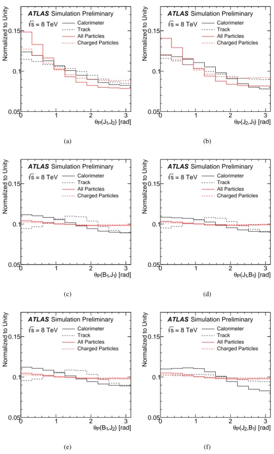
, θP

(Y, X) since the former uses the substructure properties of X while the latter uses the substructure properties of Y. Figures 3a-3f show the pull angle distributions for all cases that involve the W daughter jets and the leading b-jet B

₁

. The truth-level distributions are consistent with the corresponding truth level studies in the literature, where a peak at zero corresponds to jets which are ‘colour-connected’ (e.g. the daughters of the colour singlet W boson) and a uniform distribution corresponds to jets without such a connection [2].

Even though the truth level distributions in Figures 3c-3f are nearly flat, all of the reconstructed shapes are non-uniform. However, there are clear trends: the track pull has a peak at

π/2 and the

calorimeter pull is peaked at zero

⁵

. Therefore, to understand the detector response for the jet pull in t¯ t, it su

ffi

ces to study the truth to reconstructed jet pull angle transitions in Fig. 3a and Fig. 3d which are representative of the possible shapes and distortions in Fig. 3. To minimise the dependence on the physics processes creating the peak at zero in Fig. 3a, most of the discussion will be focused on Fig. 3d where any departure from a uniform distribution provides insight into detector e

ff

ects.

4The transverse mass,mT, is defined asm²_T=2p^lep_T E^miss_T (1−cos(∆φ)), where∆φis the azimuthal angle between the lepton and the missing transverse momentum direction. The quantityp^lep_T is the transverse momentum of the charged lepton.

5An exception is Fig. 3f for which the peaks are slightly shifted. This is due to the dependence of the pull angle on the jet pT; with a higherpTcut, Fig. 3f resembles Fig. 3d.

(6)

) [rad]

,J2

(J1

θP

0 1 2 3

Normalized to Unity

0.05 0.1 0.15

ATLAS Simulation Preliminary = 8 TeV

s Calorimeter

Track All Particles Charged Particles

(a)

) [rad]

,J1

(J2

θP

0 1 2 3

Normalized to Unity

0.05 0.1 0.15

s Calorimeter

(b)

) [rad]

,J1

(B1

θP

0 1 2 3

Normalized to Unity

0.05 0.1 0.15

s Calorimeter

(c)

) [rad]

,B1

(J1

θP

0 1 2 3

Normalized to Unity

0.05 0.1 0.15

s Calorimeter

(d)

) [rad]

,J2

(B1

θP

0 1 2 3

Normalized to Unity

0.05 0.1 0.15

s Calorimeter

(e)

) [rad]

,B1

(J2

θP

0 1 2 3

Normalized to Unity

0.05 0.1 0.15

s Calorimeter

(f)

Figure 3: The jet pull angle

θP

(X, Y) distribution for various choices of X and Y for truth jets and also for reconstructed level jets matched to the truth jets. For the reconstructed level jets the calorimeter pull angle uses calorimeter clusters for the jet constituents, while the track pull uses associated tracks for constituents. For the truth jets, the all particles pull angle uses all MC stable particles for the jet constituents, while the charged particle pull uses charged MC stable particles for constituents.

5

(7)

4.2 Jet Pull Angle Response

The transition between truth and reconstructed distributions is characterised by the jet pull angle re- sponse, R(θ

P

) – the difference between the reconstructed jet pull angle and the truth jet pull angle. The calorimeter/all particles pull angle is calculated from clusters for reconstructed jets and all stable truth particles for truth jet. The track

/

charged particles pull angle uses tracks ghost-associated to the jet for reconstructed jets and charged stable particles for truth jets. The resolution of the jet pull angle is very different depending on the type of constituent used in the definition. Figure 4 shows the inclusive jet pull angle response for both the track

/

charged particle and calorimeter

/

all particles pull angles. It is evident from the different widths of the two sets of distributions in Fig. 4 that the track pull angle is measured more precisely than the calorimeter pull angle. In terms of the RMS of the jet pull angle response, this corresponds to about a 20% improved resolution of the track pull angle over the calorimeter pull angle resolution. The numbers in Fig. 4 also indicate small biases in the jet pull angle distributions. These are expected from the true reconstructed jet pull angle distributions in Fig. 3, which show asymmetric shape deformations compared to the corresponding truth level distributions.

[rad]

θP - Truth θP

) = Reco θP

R(

-3 -2 -1 0 1 2 3

Arbitrary Units

0 0.5 1 1.5

2 2.5 3

) ,J2

(J1

θp

Track ) ,B2

(J1

θp

Track

) ,J2

(J1

θp

Calorimeter ) ,B2

(J1

θp

Calorimeter

Response Mean; RMS 0.02; 0.88 -0.01; 0.86 0.07; 1.08 -0.05; 1.08

ATLAS Simulation Preliminary

= 8 TeV s

Figure 4: The distribution of the jet pull angle response, R(θ

P

), for both

θP

( J

₁,

J

₂

) and

θP

(J

1,

B

₁

) as well as for the calorimeter pull angle and the track pull angle. Statistical uncertainties on the mean and RMS are an order of magnitude less than the values shown.

In order to fully understand the transition in shapes between truth and reconstructed in Fig. 3 more information is needed beyond the inclusive jet pull angle response from Fig. 4. There are three sources contributing to the resolution of the jet pull angle

⁶θP

(X, Y) response: the jet constituent angular resolu- tion and momentum resolution with respect to X, the angular resolution of X, and the angular resolution of Y . All angles are computed with respect to the calorimeter (all particles) jet axes, independent of the constituents used in the calculation of the (truth) jet pull angle. The considerations so far have treated all the resolutions inclusively. It is di

ffi

cult to systematically remove the resolution from the jet constituents, but it is straightforward to study the effect of the jet angular resolution on the jet pull angle.

One measure of the jet angular resolution is

σ^match

: the

∆

R between reconstructed jets and matched

6For the track-based pull, the definition also introduces some resolution. For instance,Ksdecays and photon conversions that occur before/inside the pixel detector contribute to reconstructed tracks, but are not in the list of stable MC charged particles.

Also, thepT >500 track threshold is not applied to the MC particles. All three of these effects have been studied and found to have a very small impact on the resolution and a negligible impact on the pull angle distribution shape.

(8)

truth jets

⁷

. Figure 5 shows the impact setting

σ^match =

0 by systematically replacing reconstructed jet axes with the corresponding matched truth jet axes. For both the calorimeter and track pull angles

θP

(J

1,

B

₁

), setting

σ^match =

0 of the b-jet has essentially no influence on the jet pull angle distribution due to the large lever-arm spanned by the vector connecting B

₁

and J

₁

. However, setting

σ^match=

0 of the J

₁

axis has a dramatic impact on the pull distribution shape. For the calorimeter pull, setting

σ^match =

0 of the J

₁

axis shifts the peak of the distribution to

π/2 instead of at 0. Since the track angular resolution is

much better than the calorimeter cluster angular resolution, the track pull angle resolution is dominated by the calorimeter jet angular resolution. By setting

σ^match =

0, the pull angle response RMS decreases and Fig. 5b shows that the jet pull angle distribution is nearly the same as the truth distribution.

) [rad]

,B1

(J1

θp

Calorimeter Pull Angle

0 0.5 1 1.5 2 2.5 3

Normalized to Unity

0.05 0.06 0.07 0.08 0.09 0.1 0.11 0.12 0.13 0.14 0.15

Truth Truth, B1

J1

Reco Truth, B1

J1

Reco Reco, B1

J1

Truth Reco, B1

J1

Truth Pull

= 8 TeV s

(a)

) [rad]

,B1

(J1

θp

Track Pull Angle

0 0.5 1 1.5 2 2.5 3

Normalized to Unity

0.05 0.06 0.07 0.08 0.09 0.1 0.11 0.12 0.13 0.14 0.15

Truth Truth, B1

J1

Reco Truth, B1

J1

Reco Reco, B1

J1

Truth Reco, B1

J1

Truth Pull

= 8 TeV s

(b)

Figure 5: The

θP

( J

₁,

B

₁

) distribution for the calorimeter (a) and track (b) pull angle after replacing reconstructed jet axes by truth jet axes.

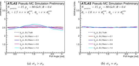
Figure 5b suggests a simple model for building intuition for the peak at

π/2. Consider a

pseudo MC model with N massless particles generated randomly from the decay of a single scalar particle whose mass and boost are tuned so that the lab frame p

_T

of the sum of the decay products is specified and such that all the decay products fall within

∆

R

<

R of the ‘jet’ axis, defined by the vector sum of all the decay products. The dashed line in figure 6 shows the jet pull angle distribution for such a model in which two such jets are generated randomly, and with N

=

10, p

_T =

80 GeV, and R

=

0.4. As expected for the undistorted distribution, the jet pull angle is uniform on [0, π). To model the resolution, the constituents are fixed and the jet axis is smeared according to a bivariate normal distribution with zero correlation and

σ^nom_φ , σ^nom_y

taken from the ATLAS detector simulation:

σ^nom_φ ≈

0.025

≈ σ^nom_y /1.5. The resolution

used in the simulation is given by

σ_φ =

r

×σ^nom_φ , σ_y =

r

×

a

×σ^nom_y

, where r is a multiplicative factor and a is an asymmetry. Figure 6a for r

=

1 shows that the peak at

π/2 is a prediction of this simple

model. By tuning the model parameters, one learns that this feature can be explained if the resolution in

y

and resolution in

φ

are not the same in ATLAS; Fig. 6b does not peak at

π/2. The peak atπ/2 comes

from two facts: (1) in (∆

y,∆φ), the pull vector tends to be stretched towards the±∆y

axis and (2) the distribution of

∆y(

J

₁,

B

₁

) is peaked at zero and thus in (

∆y,∆φ) coordinates,

B

₁

lies on the

∆φ

axis. As r

7There are at least two contributions toσ^match: 1) the angular distortions in momentum when particles become calorimeter clusters and 2) the set of particles associated with the measured calorimeter clusters may not be the same as the particles in the matched truth jet. The former effect can be studied by systematically smearing the truth jet axis and this dominatesσ^match. The impact of increased distortions of the truth axis is discussed in the context of Fig. 6.

7

(9)

is increased so that the asymmetry is no longer relevant, the peak at

π/2 disappears in all cases⁸

.

A similar model can be created for the calorimeter pull angle, but the interpretation is less straight- forward. In particular, using the same pseudo MC model for the truth selection, the calorimeter pull angle resolution can be modelled by smearing all particles and then additionally recomputing the jet axis, since the cluster angular resolution need not be small compared to the jet angular resolution as was the case for tracks. Such a model can generically predict peaks at 0, π and with angular resolution asymmetry,

π/2, but since there is not a one-to-one matching between particles and clusters, it is not possible to map

these models onto a realistic description of the detector.

Pull Angle [rad]

0 0.5 1 1.5 2 2.5 3

Arbitrary Units

1 1.5 2 2.5 3 3.5 4

) Truth , B1

(J1

θp

) Reco r = 0.1 , B1

(J1

θp

) Reco r = 0.3 , B1

(J1

θp

) Reco r = 0.6 , B1

(J1

θp

) Reco r = 1.0 , B1

(J1

θp

ATLAS Pseudo MC Simulation Preliminary = 80 GeV, R = 0.4

= 15, pT particles

N

nom

σφ

× = r σφ nom, σφ

×

× r = 1.5 σy

(a)ση> σφ

Pull Angle [rad]

0 0.5 1 1.5 2 2.5 3

Arbitrary Units

1 1.5 2 2.5 3 3.5 4

) Truth , B1

(J1

θp

) Reco r = 0.1 , B1

(J1

θp

) Reco r = 0.3 , B1

(J1

θp

) Reco r = 0.6 , B1

(J1

θp

) Reco r = 1.0 , B1

(J1

θp

ATLAS Pseudo MC Simulation Preliminary = 80 GeV, R = 0.4

= 15, pT particles

N

nom

σφ

× = r σφ nom, σφ

×

× r = 1.0 σy

(b)ση=σφ

Figure 6: The jet pull angle constructed in a pseudo MC with various resolution settings for the jet constituents.

4.3 Kinematics and the Jet Pull Angle Response

Unlike other jet substructure variables, the jet pull angle depends not only on the orientation of con- stituents within a jet, but also the placement of jets within an event, hence the term jet superstructure.

Thus, even at truth level, the jet pull angle can depend on the relative orientations of jets in a given event.

Figure 7a shows the relationship between the truth jet pull angle

θP

(J

₁,

J

₂

) and the relative distance be- tween jets,

∆

R(J

1,

J

₂

). The truth level distribution shows a strong dependence on

∆

R, with smaller values of

∆

R corresponding to a larger peak at zero. In fact, it is mostly through

∆

R that the truth level distri- bution of

θP

(J

₁,

J

₂

) depends on the p

_T

of J

₁

as shown in Appendix A. The truth pull angle distributions that involve one of the b-jets are nearly independent of

∆

R. Since the jet pull angle can depend on

∆

R, it is important to know how the resolution varies with this distance. Figure 7b shows the dependence of the RMS of the jet pull angle response as a function of

∆

R(J

₁,

B

₁

), used to illustrate the

∆

R dependence because the response does not depend on p

_T

at truth level.

Even though the jet pull angle is relatively independent of p

_T

, the response RMS does scale with p

_T

. Figure 8 shows the RMS of the jet pull angle response as a function of the p

_T

of the leading W daughter jet. The RMS of the jet pull angle response improves with increasing p

_T

as the relative jet energy resolution improves with energy.

8In fact, one might be able to use such arguments to construct ameasurementof the jet angular resolution.

(10)

) [rad]

,J2

(J1

θP

Truth

0 1 2 3

Normalized to Unity

0 0.1 0.2

s

Solid: All Particles, Dashed: Charged Particles R < 1.5

∆ 0 <

R < 2.5

∆ 1.5 <

R > 2.5

∆

(a)θP(J1,J2) in three bins of the∆R(J1,J2).

1)

1,B

∆R(J

1 1.5 2 2.5 3

RMS of Pull Angle Response [rad]

0 0.2 0.4 0.6 0.8 1 1.2 1.4 1.6 1.8

) ,B1

(J1

θp

Calorimeter

) ,B1

(J1

θp

Track

= 8 TeV s > 50 GeV

J1

pT

(b) RMS of theθPresponse as a function of∆R.

Figure 7: Relationship between the jet pull angle (response) and

∆

R.

[GeV]

pT

J1

0 100 200

0 0.2 0.4 0.6 0.8 1 1.2 1.4 1.6 1.8

) ,B1

(J1

θp

Calorimeter

) ,B1

(J1

θp

Track

= 8 TeV s

Figure 8: The RMS of the jet pull angle response as a function of the jet p

_T

. 4.4 Relationship Between the Jet Pull Angle Response and Jet Constituents

As the pull vector is determined from the constituents inside a jet, the jet pull angle response could depend on the number and orientation of the constituents of J

₁

. There are many substructure variables which capture various properties of the orientation of constituents within a jet. One such property is the pull vector magnitude,

|vp

(J)

|=

X

i∈J

p

ⁱ_T|r_i|

p

_T^J ~

r

i

In dedicated phenomenological studies [2], it was shown that the pull magnitude is not useful in discrim- inating octet from singlet colour states. However, it is a useful handle on the jet pull angle resolution.

The jet pull vector magnitude can be considered a radial moment, with the radial distance

∆

R from the jet axis weighted by the fractional constituent p

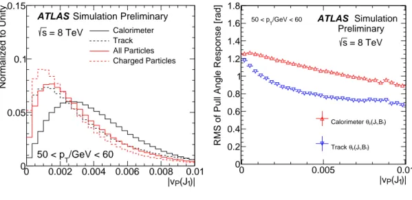
_T

. The distribution of the magnitude for J

₁

is shown

9

(11)

in the left plot of Fig. 9a. Events with a reconstructed pull vector magnitude of zero for the track pull, corresponding to cases in which there are no tracks ghost-associated to the jet, are not shown.

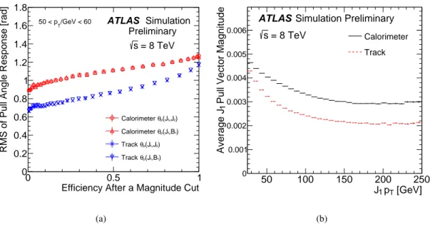
Figure 9b shows the relationship between the jet pull angle response RMS and the pull vector mag- nitude. A small pull vector magnitude corresponds to a worse resolution, in some cases because of a small lever arm. Since the pull vector magnitude can be measured, Fig. 9b suggests that events could be required to pass a threshold cut on the pull vector magnitude in order to improve precision. Figure 10a shows the RMS of the pull response as a function of the efficiency for such a cut. For instance, one can achieve a

∼10% reduction in the RMS of the jet pull angle response while maintaining a 90% selection

efficiency.

1)|

P(J

|v

0 0.002 0.004 0.006 0.008 0.01

Normalized to Unity

0 0.05 0.1 0.15

s

/GeV < 60 50 < pT

Calorimeter Track All Particles Charged Particles

(a) Pull vector magnitude.

1)|

P(J

|v

0 0.005 0.01

0 0.2 0.4 0.6 0.8 1 1.2 1.4 1.6 1.8

) ,B1

(J1

θp

Calorimeter

) ,B1

(J1

θp

Track

= 8 TeV s

/GeV < 60 50 < pT

(b) RMS ofR(θP) with|vP(J1)|.

Figure 9: (a) Pull vector magnitude and (b) the relationship between the jet pull angle (response) and

|vP

( J

₁

)| in a particular bin of jet p

_T

. For the track (charged particle) pull magnitude in the left plot, at least one track (charged particle) is required.

One undesirable property of the pull vector magnitude in terms of constraining the resolution is that it is anti-correlated with the jet p

_T

as shown in Fig. 10b. As the jet becomes more collimated, the constituents have a smaller

∆

R with respect to the jet axis and so the pull vector magnitude decreases.

Accordingly, an optimal cut on the pull vector magnitude would be p

_T

dependent. Another substructure observable that is correlated with the jet pull angle response is the number of constituents. The pull angle resolution decreases with the number of constituents at low constituent multiplicity as shown in Fig. 11.

The calorimeter pull angle and the track pull angle each require at least one cluster or track, respectively.

4.5 Jet pull angle and Event Properties

4.5.1 Jet Labeling in

t¯ t

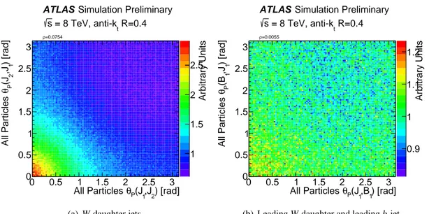
Events

For a given jet pull angle

θP

(X, Y ), there is the complimentary angle

θP

(Y

,

X) which uses different sub-

structure information. Figure 12 shows that this information is largely uncorrelated. Furthermore, it is

apparent from Figures 3a-3f that there is a relationship between the shapes of the jet pull angle distribu-

tions and the assignment of the jets in the t¯ t topology. For example, one can investigate the frequency

with which the b-tag and dijet invariant mass assignment of J

₁,

J

₂,

B

₁

and B

₂

described in Sec. 3 aligns

with the observed property that

θP

(J

₁,

J

₂

) and

θP

( J

₂,

J

₁

) tend to be smaller than

θP

(J

i,

B

j

),

θP

(B

i,

J

j

) or

(12)

Efficiency After a Magnitude Cut

0 0.5 1

0 0.2 0.4 0.6 0.8 1 1.2 1.4 1.6 1.8

) ,J2

(J1

θp

Calorimeter ) ,B1

(J1

θp

Calorimeter ) ,J2

(J1

θp

Track ) ,B1

(J1

θp

Track

= 8 TeV s

/GeV < 60 50 < pT

(a)

[GeV]

pT

J1

50 100 150 200 250

Pull Vector Magnitude1Average J

0 0.001 0.002 0.003 0.004 0.005 0.006

s Calorimeter

Track

(b)

Figure 10: (a) The RMS of the jet pull angle response as a function of the fraction of events that pass a cut on the pull vector magnitude and (b) the p

_T

dependence of the average pull vector magnitude.

Constituent Multiplicity

0 5 10

0 0.2 0.4 0.6 0.8 1 1.2 1.4 1.6 1.8

) ,B1

(J1

θp

Calorimeter

) ,B1

(J1

θp

Track

= 8 TeV s

Figure 11: The jet pull angle response as a function of the number of jet constituents for J

₁

.

θP

(B

i,

B

j

).

An event is called matched if

θP

(J

a,

J

_b

)

< θP

(J

a,

B

₁

) for any a, b

∈ {1,

2}. Conversely, if

θP

(J

a,

J

_b

)

≥ θP

(J

a,

B

₁

), an event is called un-matched. Figure 13 shows the tradeo

ff

between matched and un-matched event efficiencies for cuts on the jet pull angle using truth jets

⁹

. In other words, consider the

θP

( J

a,

J

b

) distribution as ‘signal’ and the

θP

(J

a,

B

₁

) distribution as ‘background’. Then, Fig. 13 shows the relation- ship between signal and background e

ffi

ciency as a function of the cut on

θP

. Also plotted in Fig. 13 is the combined performance curve from both variables (θ

P

(X, Y) and

θP

(Y

,

X)), which is significantly bet- ter than either curve separately. In absolute units, the overall discrimination is poor – pull is not intended

9Truth jets are used here to illustrate the maximal achievable performance in the absence of selection biases and detector resolution effects.

11

(13)

to be used as a stand-alone tagger. Since the jet pull angles with b-jets are independent of

∆

R(X, Y) but

θP

(J

₁,

J

₂

) becomes more pronounced at smaller

∆

R, there is a slight improvement in the e

ffi

ciency curve, which is shown in Fig 13b.

Arbitrary Units

1 1.5 2 2.5

) [rad]

,J2

(J1

θP

All Particles

0 0.5 1 1.5 2 2.5 3

) [rad] 1,J 2(JPθAll Particles

0 0.5 1 1.5

2 2.5 3

ATLAS Simulation Preliminary R=0.4 = 8 TeV, anti-kt

s

=0.0754 ρ

(a)Wdaughter jets.

Arbitrary Units

0.9 1 1.1 1.2

) [rad]

,B1

(J1

θP

All Particles

0 0.5 1 1.5 2 2.5 3

) [rad] 1,J 1(BPθAll Particles

0 0.5 1 1.5

2 2.5 3

ATLAS Simulation Preliminary R=0.4 = 8 TeV, anti-kt

s

=0.0055 ρ

(b) LeadingWdaughter and leadingb-jet.

Figure 12: Pairwise all particles pull angle correlations.

% Matched

0 0.2 0.4 0.6 0.8 1

1-% un-Matched

0 0.2 0.4 0.6 0.8 1

♦)

1,

P(J θ

1)

♦,J

P( θ

Optimal Combination Random Match

ATLAS Simulation Preliminary

(a) Inclusive∆R.

% Matched

0 0.2 0.4 0.6 0.8 1

1-% un-Matched

0 0.2 0.4 0.6 0.8 1

♦)

1,

P(J θ

1)

♦,J

P( θ

Optimal Combination Random Match

ATLAS Simulation Preliminary R < 1.5

∆

(b)∆R(X,Y)<1.5.

Figure 13: Un-matched event (treated as a background) rejection versus the matched (treated as a signal) efficiency. The optimal combination is constructed from the full joint likelihood.

4.5.2 Pileup

An important event property from the point of view of the pull angle RMS is

µ

- the average number of

additional pp interactions per bunch crossing at the LHC. The dependence of the RMS of the jet pull

angle response is shown as a function of

µ

in Fig. 14. The RMS of the jet pull angle response is only

(14)

weakly dependent on the pileup activity. For example, a linear fit to the data in Fig. 14 results in a slope of about (1.6

±

0.1)× 10

⁻³

rad

/

interaction for the calorimeter pull angle response RMS and (1.5± 0.1)× 10

⁻³

rad/interaction for the track pull angle response RMS in the range 50 GeV

<

p

_T^J¹ <

60 GeV . This trend does not vary greatly with p

_T

.

0 10 20 30 µ40

0 0.2 0.4 0.6 0.8 1 1.2 1.4 1.6 1.8

) ,B1

(J1

θp

Calorimeter

) ,B1

(J1

θp

Track

= 8 TeV s

/GeV < 60 50 < pT

Figure 14: The RMS of the jet pull angle response as a function of

µ

for 50 GeV

<

p

^J_T¹ <

60 GeV.

5 Jet Pull in the Data

The purpose of the following comparisons with data is to investigate the modelling of the detector per- formance of the jet pull. It is a basic validation to build confidence in the previous sections where MC was used exclusively. Detailed studies with unfolded data to compare various models of colour flow are beyond the scope of this note. This section includes comparisons of jet pull distributions in data and MC, where the reconstructed object-based selection described in Section 3 is applied to both data and MC.

The MC is normalised by area to the data in all the following distributions. The uncertainty bands on the data/MC ratios include the experimental uncertainty on the tracking efficiency, the jet energy scale and the jet energy resolution in addition to a

±6% relative uncertainty on the

t¯ t component of the MC from the cross section estimate [31–36]. For the pull angle, the average uncertainty across all bins is plotted to remove fluctuations due to the small dependence of the pull angle on the jet energy scale and resolution uncertainties. Uncertainties on the cluster energy scale and angular resolution are not included.

Since the jet pull vector magnitude shows important discrimination power against poor resolution in the jet pull angle response, the first data distribution, shown in Figure 15, is the reconstructed J

₁

pull vector magnitude. The modelling of both the calorimeter and track pull vector magnitudes are within 10% of the data over a large range of magnitude values. This conclusion also holds if a di

ff

erent shower model (PYTHIA 6 with the Perugia2011C tune) and matrix element generator (PowHeg [37–39] with PDF set CT10) are used, although unfolding studies are required to entirely disentangle physics e

ff

ects from problems with detector modelling (see Fig. 18 for the PowHeg plot). For the track pull angle, at least two tracks are required in order to remove the portion of the resolution curve in Fig. 11 where the response RMS decreases at low constituent multiplicity.

The distribution of the jet pull angle in the data is shown in Fig. 16 for

θP

( J

₁,

J

₂

). Like the pull vector magnitude, the jet pull angle is well modelled by the MC. In particular, the resolution features at

π/2 for tracks and at zero for the calorimeter pull are both present and well described. The bias toward

13

(15)

Events/0.0003

0 500 1000 1500 2000 2500

3000 ATLAS Preliminary L dt = 20 fb-1

∫

= 8 TeV, s

t

MC@NLO t Calorimeter (MC)

Track (MC) Calorimeter (Data) Track (Data)

Pull Vector Magnitude J1

TracksData/MC 0.5 1 1.5

0 0.005 0.01 0.015

CaloData/MC 0.5 1 1.5

Figure 15: The pull vector magnitude for both calorimeter pull and track pull. For the track pull, at least two tracks are required. Uncertainty bands include uncertainties on the jet energy scale and uncertainty as well as on the t¯ t component of the MC. An uncertainty on the tracking efficiency is added for the track pull. No uncertainty is included for individual calorimeter clusters or for jet angular resolutions.

zero in the truth distribution (Fig. 3) that is also present in the truth-object based selection (Fig. 3a) is reduced in Fig. 16 due to a selection bias: in a given event, the truth-based and reconstructed-based assignment of jet labels can di

ff

er. This selection bias decreases with the increasing p

_T

of the jets, as is seen in Fig. 16b, where the peak at zero for the track pull dominates the resolution peak at

π/2 in the MC.

Figure 17 shows the jet pull angle distribution between the leading W daughter jet and the leading b-jet.

Based on the studies summarised in Fig. 6, the slight trend in Fig. 17a (and Fig. 16a) suggests that the scale or asymmetry parameter of the jet angular resolution may be over-estimated, though quantifying this statement is beyond the scope of this note.

Figures 19 and 20 for the PowHeg distributions corresponding to Figures 16 and 17 show that the conclusions from the nominal t¯ t sample still hold within the uncertainties.

6 Conclusions

The studies presented in this note have used t¯ t events with one leptonically decaying W to analyze the

impact of the detector response on the jet pull angle distribution for W daughter jets and for b-jets. Since

the resolution for the jet pull angle varies with the type of constituent, the resulting reconstructed jet pull

angle shape is different for the calorimeter pull and the track pull. It has been shown that the pull vector

magnitude is useful at constraining the jet pull angle resolution and thus analyses using the jet pull angle

may consider a requirement on the magnitude. The following are the key observations described in this

note:

(16)

> 25 GeV

,B1 ,J2 J1

pT

/10 radπEvents/

3000 4000 5000 6000

∫

= 8 TeV, s

t MC@NLO t

> 25 GeV

,B1 ,J2 J1

pT

Calorimeter (MC) Track (MC) Calorimeter (Data) Track (Data)

) [rad]

,J2 (J1 θP

) [rad]

,J2 (J1 θP

0 1 2 3

(a) Inclusive

> 100 GeV

+J2 J1

pT

/10 radπEvents/

400 600 800 1000 1200 1400 1600

∫

= 8 TeV, s

t MC@NLO t

> 100 GeV

+J2 J1

pT

) [rad]

,J2 (J1 θP

) [rad]

,J2 (J1 θP

0 1 2 3

(b) High dijetpT

Figure 16: The distribution of the jet pull angle

θP

(J

1,

J

₂

) for both calorimeter cluster constituents and track constituents in both data and MC. The left plot has a 25 GeV requirement for the jets while the right plot has a tight threshold placed on the p

_T

of the dijet system. Uncertainty bands include uncertainties on the jet energy scale and uncertainty as well as on the t¯ t component of the MC. An uncertainty on the tracking e

ffi

ciency is added for the track pull. No uncertainty is included for individual calorimeter clusters or for jet angular resolutions.

•

While the non-trivial features in the

θP

(J

₁,

J

₂

) distribution are more pronounced for the calorimeter pull, the pull angle resolution is better for the track pull. Practically, this means that the calorimeter pull has more discriminating power, but the track pull has a closer-to-diagonal response matrix.

•

The reconstructed track pull shape (peak at

π/2) for θP

( J

₁,

B

₁

) can be understood in terms of detector geometry.

•

For every measured pull angle

θP

(X, Y), there is another angle

θP

(Y, X) that uses largely uncorre- lated information.

•

The pull angle and pull vector magnitude in the data are well-modelled by the MC.

With the detector performance at hand, it will now be interesting to see how the jet pull angle per- forms in the variety of analyses to which it might be useful e.g. searches or measurements involving the colour singlet bosons W, Z and/or H.

15

(17)

> 25 GeV

,B1 ,J2 J1

pT

/10 radπEvents/

2000 2500 3000 3500 4000 4500 5000 5500 6000

∫

= 8 TeV, s

t MC@NLO t

> 25 GeV

,B1 ,J2 J1

pT

) [rad]

,B1 (J1 θP

) [rad]

,B1 (J1 θP

0 1 2 3

(a) Inclusive

> 100 GeV

+B1 J1

pT

/10 radπEvents/

400 600 800 1000 1200 1400 1600 1800 2000

∫

= 8 TeV, s

t MC@NLO t

> 100 GeV

+B1 J1

pT

) [rad]

,B1 (J1 θP

) [rad]

,B1 (J1 θP

0 1 2 3

(b) High dijetpT

Figure 17: The distribution of the jet pull angle

θP

(J

₁,

B

₁

) for both calorimeter cluster constituents and

track constituents in both data and MC. The left plot has a 25 GeV requirement for the jets while the right

plot has a tight threshold placed on the p

_T

of the dijet system. Uncertainty bands include uncertainties

on the jet energy scale and uncertainty as well as on the t¯ t component of the MC. An uncertainty on

the tracking efficiency is added for the track pull. No uncertainty is included for individual calorimeter

clusters or for jet angular resolutions.

(18)

Events/0.0003

0 500 1000 1500 2000 2500

∫

= 8 TeV, s

t

POWHEG t Calorimeter (MC)

Track (MC) Calorimeter (Data) Track (Data)

0 0.005 0.01 0.015

Figure 18: The pull vector magnitude for both calorimeter pull and track pull. For the track pull, at least two tracks are required. Uncertainty bands include uncertainties on the jet energy scale and uncertainty as well as on the t¯ t component of the MC. An uncertainty on the tracking e

ffi

ciency is added for the track pull. No uncertainty is included for individual calorimeter clusters or for jet angular resolutions. This plot corresponds to Fig. 15, but the POWHEG simulation is used instead of MC@NLO.