ATLAS-CONF-2019-026 17/09/2021
ATLAS CONF Note
ATLAS-CONF-2019-026
11th July 2019
Inclusive and differential measurements of the charge asymmetry in t t ¯ events at 13 TeV with the
ATLAS detector
The ATLAS Collaboration
A measurement of the top-antitop (
tt¯ ) charge asymmetry
ACis presented using data corres- ponding to an integrated luminosity of 139 fb
−1of
√s=
13 TeV of
ppcollisions recorded by the ATLAS experiment at the Large Hadron Collider, CERN. The measurement is performed in the single-lepton channel (
eor
µ) combining both the resolved and boosted topologies of top quark decays. A Bayesian unfolding procedure is used to infer the asymmetry at parton level, correcting for detector resolution and acceptance effects. The inclusive
t¯tcharge asymmetry is measured as
AC =0
.0060
±0
.0015(stat+syst.), which differs from zero by 4 standard deviations. Differential measurements are performed as a function of the invariant mass and longitudinal boost of the
t¯tsystem. Both inclusive and differential measurements are found to be compatible with the Standard Model predictions, at NNLO in perturbation theory with NLO electroweak corrections.
© 2021 CERN for the benefit of the ATLAS Collaboration.
Reproduction of this article or parts of it is allowed as specified in the CC-BY-4.0 license.
1 Introduction
The large mass of the top quark, which is close to the electroweak symmetry breaking scale, indicates that this particle could play a special role in the Standard Model (SM) as well as in beyond the Standard Model (BSM) theories. Due to the high top-pair production (
t¯t) cross section for 13 TeVproton–proton (
pp) collisions [1], the Large Hadron Collider (LHC) experiments collect an unprecedented number of events in which a
tt¯ pair is produced. The top quark has a very short lifetime (
τt ≈0
.5
×10
−24s) and decays before hadronisation (
τhad ∼10
−23s), therefore, several of its properties may be measured precisely from studies of the top quark’s decay products. These measurements probe predictions of quantum chromodynamics (QCD), which provides the largest contribution to
t¯tproduction. They also probe potential contributions from couplings between the top quark and BSM particles [2–4].
Production of top quark pairs is symmetric at leading-order (LO) under charge conjugation. The asymmetry between the
tand ¯
toriginates from interference of the higher-order amplitudes in the
qq¯ and
qginitial states, with the
qq¯ annihilation contribution dominating. The contribution from electro-weak corrections is about 13% for the inclusive asymmetry and almost 20% for high
mtt¯bins [5–7] in the differential case.
The
qg→ttg¯ production process is also asymmetric, but its cross section is much smaller than
qq¯ . Gluon fusion production is symmetric to all orders. As a consequence of these asymmetries, the top quark is preferentially produced in the direction of the incoming quark.
At a
pp¯ collider, where the preferential direction of the incoming quark (antiquark) always almost coincides with that of the proton (anti-proton), a forward-backward asymmetry
AFBcan be measured directly [8–11].
At the LHC
ppcollider, since the colliding beams are symmetric, it is not possible to measure
AFBas there is no preferential direction of either the top quark or the top antiquark. However, due to the difference in the proton parton distribution functions, on average the valence quarks carry a larger fraction of the proton momentum than the sea antiquarks. This results in more forward top quarks and more central top antiquarks. A central–forward charge asymmetry for the
t¯tproduction, referred to as the charge asymmetry (
AC) is defined as [8, 12, 13]:
AC = N(∆|y| >
0
)−N(∆|y| <0
)N(∆|y| >
0
)+N(∆|y| <0
),(1) where
∆|y|= |yt| − |yt¯|is the difference between the absolute value of the top-quark rapidity
|yt|and the absolute value of the top-antiquark rapidity
|yt¯|. At the LHC, the dominant
t¯tproduction mechanism is via gluon fusion, especially for collisions with higher centre of mass energy. The contributions from
qq¯ and
qgare small, so the charge symmetric
gg→tt¯ process dilutes the measureable asymmetry.
Several BSM processes, such as anomalous vector or axial couplings (e.g. axigluons), heavy
Z’ bosons, or processes which interfere with the SM can alter
AC[2–4, 12, 14–21]. Several BSM models predict charge asymmetries which vary as a function of the invariant mass
mtt¯and the longitudinal boost of the
t¯tsystem along the
z-axis
βz,tt¯.1 In particular, BSM effects are expected to be enhanced in specific kinematic regions, for example, when the
βz,tt¯or
mtt¯are large [22]. Previously the CDF and D0 collaborations reported measurements of
AFBlarger than the LO SM prediction [10, 11, 23–26], however these are in
1ATLAS uses a right-handed coordinate system with its origin at the nominal interaction point (IP) in the centre of the detector and thez-axis along the beam pipe. Thex-axis points from the IP to the centre of the LHC ring, and they-axis points upwards.
Cylindrical coordinates(r, φ)are used in the transverse plane,φbeing the azimuthal angle around thez-axis. The pseudorapidity is defined in terms of the polar angleθasη=−ln tan(θ/2). Angular distance is measured in units of∆R≡
q
(∆η)2+(∆φ)2.
agreement with higher orders calculations. The measurements performed so far by both the ATLAS and CMS collaborations at
√s
=7, 8 and 13 TeV, in different decay channels and topologies, have demonstrated good agreement with SM predictions [27–37].
However, even for the combined ATLAS and CMS inclusive and differential measurements in lepton+jet channel at
√s=
7 and
√s=
8 TeV [38], uncertainties in kinematic regions such as high
mtt¯are statistically dominated and do not have the sensitivity to exclude BSM signals.
This document reports the measurement of
ACin
t¯tproduction with 139 fb
−1of data at
√s =
13 TeV recorded by the ATLAS experiment at the LHC. The measurement is made in
tt¯ events with a single isolated lepton in final state (lepton+jets), in both the resolved and boosted topologies of the top quark decays. The measurements in both topologies are combined and
ACis measured inclusively, as well as differentially as a function of the
mtt¯and
βz,t¯t. A Bayesian unfolding procedure [39] is applied to correct for acceptance and detector effects, resulting in parton-level
ACmeasurements for comparison with theory calculations. This measurement exploits the large amount of data in two ways: reducing the statistical uncertainty and constraining the large uncertainties in-situ.
The document is organised as follows. The ATLAS detector is described in Section 2, and the object definitions and event selections are detailed in Sections 3 and 4, respectively. The signal and background modelling and the estimation of the fake lepton backgrounds are described in Section 5. The unfolding procedure is presented in Section 6. Section 7 discusses the systematics uncertainties, and the results are summarised in Section 8 with conclusions drawn in Section 9.
2 ATLAS detector
The ATLAS detector [40] covers nearly the entire solid angle around the collision point. It consists of an inner tracking detector (ID) surrounded by a thin superconducting solenoid, electromagnetic (EM) and hadronic calorimeters, and a muon spectrometer (MS), incorporating three large superconducting toroidal magnets. The ID is immersed in a 2 T axial magnetic field and provides charged-particle tracking in the range
|η| <2
.5.
The high-granularity silicon pixel detector covers the proton collision region and typically provides four measurements per track. The first layer is the insertable B-layer (IBL), which was installed prior to 2015 data taking [41, 42]. Outside of this is the silicon microstrip tracker (SCT) which records up to eight measurements per track. These silicon detectors are complemented by the transition radiation tracker (TRT), which provides radially extended track reconstruction up to
|η|=2
.0. The TRT also produces electron identification information based on the fraction of hits (typically 30 in total) above an energy-deposit threshold corresponding to transition radiation.
The calorimeter system covers the pseudorapidity range
|η| <4
.9. Within the region
|η| <3
.2, EM
calorimetry is provided by high-granulairty barrel and endcap lead/liquid-argon (LAr) calorimeters, with
an additional thin LAr presampler covering
|η| <1
.8, to correct for energy loss in material upstream of the
calorimeters. Hadronic calorimetry is provided by a steel/scintillating-tile calorimeter, which is segmented
into three barrel structures within
|η|<1
.7, and two copper/LAr hadronic endcap calorimeters. The solid
angle coverage is completed with forward copper/LAr and tungsten/LAr calorimeter modules optimised for
EM and hadronic measurements respectively.
The MS comprises separate trigger and high-precision tracking chambers. These measure the deflection of muons in a magnetic field generated by superconducting air-core toroids. The field integral of the toroids ranges between 2.0 and 6.0 T m across most of the detector. Tracking chambers cover the region
|η| <2
.7 consisting of three layers of monitored drift tubes, which are complemented by cathode-strip chambers in the forward region where the background is highest. The muon trigger system covers the range
|η| <2
.4 with resistive-plate chambers in the barrel, and thin-gap chambers in the endcap regions. Interesting events are selected to be recorded by the first-level (L1) trigger system using custom hardware. This is followed by selections made using algorithms implemented in software in the high-level trigger (HLT) [43]. The L1 trigger reduces the 40 MHz bunch crossing rate to below 100 kHz. The HLT further reduces this rate in order to record events to disk at 1 kHz.
3 Object definition and reconstruction
This analysis utilises reconstructed electrons, muons, jets,
b-jets, large-radius (large-
R) jets and missing transverse momentum.
The primary vertex (PV) of an event is that which has the highest
P ptrackT
[44], where the sum extends over all associated tracks with
pT >0
.5 GeV. At least two tracks are required.
Electron candidates are reconstructed from clusters in the EM calorimeter that are associated to tracks in the inner detector [45]. Candidates are required to have a transverse energy,
ET, greater than 28 GeV and
|ηcluster| <
2
.47. If
ηclusteris within the transition region between the barrel and the end-cap of the LAr calorimeter (1
.37
< |ηcluster| <1
.52) the electron candidate is removed. A multivariate algorithm is used to select signal electrons, which have to satisfy a “tight” likelihood-based quality criterion. Additional impact parameter criteria applied are
|d0|/σ(d0) <5 and
|z0sin
θ| <0
.5 mm. The electron candidates have to pass
pT- and
η-dependent isolation requirements based on their tracks and clusters, which results in an electron reconstruction efficiency of 90% at
pT=25 GeV and 99% at
pT =60 GeV.
Muon candidates are reconstructed from ID tracks combined with track segments or full tracks in the MS [46]. Candidates are required to fulfill the “medium” identification quality criteria. Only muon candidates within
|η| <2
.5,
pT >28 GeV, and with impact parameter criteria of
|d0|/σ(d0) <3 and
|z0
sin
θ| <0
.5 mm, are selected. For muon candidates, the track isolation is defined similarly to electron candidates and the average identification efficiency is 98% as measured on data.
Jets are reconstructed with the anti-
ktalgorithm [47] using a radius parameter
R =0
.4 (small-
R) from calibrated topological calorimeter clusters [48]. The jet calibration relies on Monte Carlo (MC) simulations, with additional corrections obtained using in-situ techniques to correct for differences observed between simulations and data. The jet energy is corrected for pile-up effects using a jet area method [49] and further corrected using a calibration based on both MC simulations as well as data [50]. Only jets with
pT >25 GeV and within the central region are selected. Additionally, a Jet Vertex Tagger (JVT) [51]
is used to discriminate between jets originating from the PV and from pile-up collisions, for jets with
pT <60 GeV and
|η| <2
.4. The selected JVT working point provides an average efficiency of 92% for hard-scatter jets and a rejection factor of 99% for pile-up jets.
Jets containing
b-hadrons are identified (‘
b-tagged’) using a multivariate algorithm. Inputs are combined
from algorithms which use secondary vertices reconstructed within a jet and track impact parameters [52,
53]. For this measurement, the operating point corresponds to a 77% efficiency to tag
b-quark jets,
with a purity of 95%. The corresponding rejection factors for jets originating from a
c-quark, light
quark or
τlepton are 5, 100, and 20, respectively. To account for possible mismodelling between data and predictions of the selection efficiencies for the different quark flavour jets and jets originating from hadronically-decaying
τleptons, per-jet scale factors are obtained from
tt¯ events in data [53, 54].
Large-
Rjets are reconstructed with the anti-
ktalgorithm [47] from the individually-calibrated topological cell clusters [50, 55], using a radius parameter
R =1
.0 and calibrated from simulation [56]. They are subsequently trimmed [57] to remove the effects of pile-up and underlying event. Trimming is a technique in which the original constituents of the jets are reclustered using the
ktalgorithm [58] with a distance parameter
Rsub, in order to produce a collection of sub-jets. Sub-jets with a fraction of the large-
Rjet
pTless than a calibrated threshold
fcutare removed. The trimming parameters used here are
Rsub=0
.2 and
fcut=5% based on previous studies [59]. The large-
Rjet moments (e.g. mass,
τ322) are calculated usingonly the constituents of the selected sub-jets.
The missing transverse momentum [61], with magnitude
EmissT
, is calculated from a vectorial sum of all reconstructed objects. The calculation utilises calibrated electrons, muons, photons, hadronically decaying
τ-leptons, and jets reconstructed from calorimeter energy deposits. These are combined with soft hadronic activity measured by reconstructed charged-particle tracks not associated to other hard objects.
In order to avoid double counting of the same energy clusters or tracks as different object types, an overlap removal procedure is applied. First, electron candidates sharing a track with any muon candidates are removed. Secondly, if the distance between a small-
Rjet and an electron candidate is
∆R<0
.2, the jet is removed. If multiple small-
Rjets are found with this requirement, only the closest small-
Rjet is removed.
If the distance between a small-
Rjet and an electron candidate is 0
.2
< ∆R <0
.4, then the electron candidate is removed. If the distance between a small-
Rjet and any muon candidates is
∆R<0
.4, the muon candidate is removed if the small-
Rjet has more than two associated tracks, otherwise the small-
Rjet is removed. Finally, if the distance between a large-
Rjet and the electron candidate is
∆R<1
.0, the large-
Rjet is removed.
4 Event selection and reconstruction
The analysis uses data collected by the ATLAS detector between 2015 and 2018 from
ppcollisions at a centre-of-mass energy of
√s =
13 TeV, corresponding to an integrated luminosity of 139 fb
−1. Only events recorded under stable beam conditions with all detector subsystems operational, with a primary vertex and passing a single-electron or single-muon trigger are considered. Multiple triggers are used to increase the selection efficiency. The lowest-threshold triggers utilise isolation requirements to reduce the trigger rate. These have
pTthresholds of 20 GeV for muons and 24 GeV for electrons in 2015 data, and 26 GeV for both lepton types in 2016, 2017 and 2018 data. They are complemented by other triggers with higher
pTthresholds and with no isolation requirements in order to increase event acceptance.
A common event selection is used for the resolved and boosted topologies, requiring exactly one lepton candidate matched to the trigger lepton with a minimum transverse momentum of 28 GeV. Events containing additional leptons with transverse momentum larger than 25 GeV are rejected. To reduce the impact of the multijet background, cuts on
EmissT
and
MWT
are applied
3. In the electron channel, bothEmissT
and
MWT
are required to be larger than 30 GeV because of the higher level of multijet background (see
2theτ32is defined in Ref. [60]
3MW
T =q 2p`
TEmiss
T (1−cos∆φ)where∆φis the angle between the lepton andEmiss
T in the transverse plane.
Sec. 5.4), while in the muon channel a triangular cut
EmissT +MW
T >
60 GeV is applied. At least one of the small-
Rjets is required to be
b-tagged. The selected events are further divided into 1
b-tag-exclusive and 2
b-tag-inclusive regions based on the
b-jet multiplicity, while the electron and muon channels are summed.
4.1 Event selection and reconstruction in the resolved topology
The resolved topology requires at least four small-
Rjets with
pT >25 GeV. The
tt¯ system is reconstructed using a boosted decision tree (BDT) algorithm to find the correct assignment of the reconstructed final state objects to the
t¯tdecay products. Events which also pass the boosted selection are removed.
The challenge of reconstructing an event in the resolved topology is to correctly assign individual selected jets to the corresponding partons from the decaying top-quarks. For this purpose, an multivariate technique implemented within the
TMVApackage [62] is designed. The BDT combines kinematic event variables and
b-tagging information, with weight information from the Kinematic Likelihood Fitter (KLFitter) [63], into a single discriminant. Each permutation of jet-to-parton assignments is evaluated and the permutation with the highest BDT score is used for the
t¯tkinematic reconstruction.
Since the number of possible permutations rapidly increases with the jet multiplicity, only permutations of up to five jets are considered. If more than five jets are present in an event, the two highest
b-tagging score jets are considered, together with the remaining three highest
pTjets. The
t¯tsignal sample (see Sec. 5.1) is used for the BDT training, while each jet-to-parton permutation is flagged as either "signal" or
"background". Only permutations with four jets correctly assigned within
∆R=0
.3 of the corresponding partons are flagged as signal, all other permutations are considered as combinatorial background. There is no attempt to correctly match the individual partons from the hadronically decaying
Was it does not affect the reconstruction. The BDT aims to discriminate the signal from the combinatorial background and is trained separately for the 1
b-exclusive and 2
b-inclusive
b-tag regions, but inclusively in the lepton flavour (electron, muon). The BDT is trained using only the background permutations with a significant probability of being mistakenly identified as signal, which are the ones for which the KLFitter calculates the highest likelihood.
Thirteen variables are used as input to the BDT:
• the reconstructed mass of the hadronically-decaying top quark,
• the logarithm of likelihood from the KLFitter,
• the reconstructed mass of the hadronically-decaying
Wboson,
•
b-tagging information for the
b-jet from the semileptonically-decaying top quark,
• the
b-jet from the hadronically-decaying top quark,
• the light-jet from the
Wboson decay,
• the reconstructed mass of the semileptonically-decaying top quark,
• the
∆Rbetween
b-jet from semileptonically-decaying top quark and lepton,
• the
∆Rbetween the two light jets from
Wdecay,
• the
pTof the lepton and
b-jet from semileptonically-decaying top quark,
• the number of jets in the event,
• the pseudorapidity of the hadronically-decaying top quark,
• and finally the
∆Rbetween the two
b-jets from
t¯tdecay.
For the final selection, events are required to have a BDT discriminant for the best permutation with a score
>
0
.3 in order to reject
tt¯ combinatorial backgrounds and suppress non-
t¯tbackground processes as they naturally populate low regions of BDT since no permutation matches expected kinematics of
t¯t. Using the lower threshold on the BDT discriminant increases the signal to non-
t¯tbackground ratio by a factor of
∼2.
In addition, for
t¯tsignal events where a jet-to-parton assignment is possible for all partons from
t¯tdecay, the correct assignment is found for 75% of the events.
4.2 Event selection and reconstruction in the boosted topology
In the boosted topology, the reconstruction aims to identify one high
pTand collimated hadronic top-quark decay and at least one small-
Rjet with
pT >25 GeV close to the selected lepton with
∆R(jet
R=0.4,
`) <1
.5.
If multiple small-
Rjets satisfy this condition, the one with highest
pTis considered for the subsequent boosted top quark reconstruction. In addition, at least one large-
Rtop-tagged jet with
pT >350 GeV and
|η| <2 is required as the hadronically-decaying top quark. Since both top quarks are expected to be back-to-back in the
t¯trest frame, additional cuts related to the large-
Rjet, the isolated lepton and the small-
Rjet close to the lepton are applied:
∆φ(jet
R=1.0,
`) >2
.3 and
∆R(jet
R=1.0, jet
R=0.4) >1
.5. The large-
Rjet is evaluated by a top-tagging algorithm utilising jet mass and
τ32substructure [60] variables, where an operating point with an efficiency of 80% is chosen. The top tagger is optimised using the same approach as described in Ref. [64]. Finally, a cut on the invariant mass of the reconstructed
t¯tsystem of
mtt¯>500 GeV is applied. This criterion is imposed to remove a negligible fraction (0.1%) of poorly-reconstructed events which pass the boosted selection criteria above. In addition, this removes the lowest
mt¯tbin in the corresponding differential
ACmeasurement which would suffer from extremely low statistics.
The four-momentum of the leading-
pTlarge-
Rjet satisfying the selection criteria is taken as the four- momentum estimate of the hadronically-decaying top quark. The semileptonically-decaying top-quark four-momentum is constructed from the isolated lepton, the selected small-
Rjet and the neutrino four- momentum. The neutrino four-momentum is calculated using the constraints from the
EmissT
value, the lepton kinematics and the
Wboson mass. If there are two possible solutions for the neutrino four-momentum, the solution with the minimum
|pz|is chosen. If there is no real solution, the
EmissT
vector is varied in the transverse plane by the minimum amount necessary to obtain at least one solution.
5 Signal and background modelling
All signal and background processes are modelled using MC simulations, with the exception of non-prompt lepton and non-leptonic particle (fake lepton) backgrounds, which are estimated from data (see Sec. 5.4).
All simulated samples use EvtGen v1.6.0 [65] to model the decays of heavy hadrons, with the exception
of the background samples generated with Sherpa [66]. Most of the MC samples are processed using
a full simulation of the detector response with the GEANT4 toolkit [67]. The samples used to estimate
modelling systematic uncertainties are either obtained by reweighing the default full simulation samples, or
are produced using fast simulation software ATLFASTII [68]. To model additional
ppinteractions from the same or neighbouring bunch crossings, the hard scattering events are overlaid with a set of minimum-bias interactions generated using Pythia8 [69] and the MSTW2008LO [70] parton distribution function (PDF) set with the A3 [71] tuned parameter settings. Finally, the simulated MC events are reconstructed using the same software as the data. Detailed explanations on the MC samples for the signal and for each background are provided in the following.
5.1 t t ¯ signal
All
t¯tsamples, except for mass variation samples, assume a top-quark mass of
mtop=172
.5 GeV and are normalised to the inclusive production cross section of
σ(tt)¯
=832
±51 pb. This cross section is calculated at next-to-next-to-leading order (NNLO) in QCD including the resummation of next-to-next-to-leading logarithm (NNLL) soft-gluon terms using Top++2.0 [72–78]. The uncertainties on the cross-section due to PDF and
αsare calculated using the PDF4LHC prescription [79] with the MSTW2008 68% CL NNLO [70, 80], CT10 NNLO [81, 82] and NNPDF2.3 5f FFN [83] PDF sets, and are added in quadrature to the scale uncertainty.
The nominal
t¯tevents are generated with the PowhegBox [84–87] v2 generator which provides matrix elements at next-to-leading order (NLO) in the strong coupling constant
αS, with the NNPDF3.0NLO [88]
PDF and the
hdampparameter4 set to 1
.5
mtop[89]. The functional form of the renormalisation and factorisation scales (
µrand
µf) is set to the nominal scale of
q m2
top+p2
T
. The events are interfaced with Pythia8.230 for the PS and hadronisation, using the A14 set of tuned parameters [90] and the NNPDF23LO PDF set.
To study the
t¯tmodelling uncertainties, alternative samples which use the ATLFASTII simulation are considered.
The uncertainty due to initial-state-radiation (ISR) is estimated from an altered
t¯tsample with variations in the additional radiation [91]. To simulate higher parton radiation,
µrand
µfare varied by a factor of 0.5 while simultaneously increasing the
hdampvalue to 3
mtop. The nominal
t¯tsignal sample is used to estimate reduced initial-state radiation, by varying the scales by a factor of 2.0 using weights. The impact of final-state-radiation (FSR) is evaluated using PS weights in Pythia8, for the up and down variations the renormalisation scale for QCD emission in FSR is altered factors of 0.5 and 2.0, respectively.
The impact of the PS and hadronisation model is evaluated using the nominal generator, but interfaced with Herwig7.04 [92, 93] using the H7UE set of tuned parameters [93], and the MMHT2014LO PDF set [94].
To assess the uncertainty due to the choice of the matching scheme MadGraph5_aMC@NLO (referred to as MG5_aMC in the following) [95] and Pythia8 is used. The calculation of the hard-scattering uses MG5_aMC v2.6.0 with the NNPDF3.0NLO [88] PDF set. Events are interfaced with Pythia8.230 [69], using the A14 set of tuned parameters [90] and the NNPDF23LO PDF. The shower starting scale has the functional form
µq =HT/2 [91], where
HTis defined as the scalar sum of the
pTof all outgoing partons.
The renormalisation and factorisation scale choice is the same as used with Powheg .
4Thehdampparameter controls the transverse momentumpTof the first additional emission beyond the LO Feynman diagram in the parton shower (PS) and therefore regulates the high-pTemission against which thett¯system recoils.
To study the effect on
ACof different values of the top-quark mass, two samples are generated using the same settings as in the nominal
t¯tsignal sample (Powheg + Pythia8), but with
mtopset to either 172 GeV or 173 GeV.
Finally, the PROTOS generator [96] with the CTEQ6L1 PDF set is used to generate
tt¯ samples predicting different asymmetry values due to the inclusion of a new heavy axigluon. The generated samples contain only parton level information, which is later used to re-weight the nominal
t¯tPowheg +Pythia8 sample.
5.2 Single top
Single-top
tWassociated production is modelled using the PowhegBox [85–87, 97] v2 generator which provides matrix elements at NLO in
αS, using the five flavour scheme with the NNPDF3.0NLO [88] PDF set. The functional form of
µrand
µfis set to the nominal scale of
q m2
top+p2
T
. The diagram removal scheme [98] is employed to treat the interference with
t¯tproduction [89]. Dedicated samples with a diagram subtraction (DS) scheme [98] are considered to evaluate the uncertainty due to the treatment of the overlap with
tt¯ production.
Single-top
t-channel (
s-channel) production is modelled using the PowhegBox [85–87, 99, 100] v2 generator which provides matrix elements at NLO in
αS, using the four (five) flavour scheme with the NNPDF3.0NLO [88] PDF set. The functional form of
µrand
µfis set to
q m2
b+p2
T,b
[99].
For these processes, the events are interfaced with Pythia8.230 [69] using the A14 tune [90] and the NNPDF23LO PDF set.
The uncertainty due to ISR is estimated using varied weights in the matrix element (ME) and in the PS. To simulate higher ISR,
µrand
µfare varied by a factor of 0.5 in the ME. For the simulation of lower ISR,
µrand
µfare varied by a factor of 2.0. The impact of increased or decreased FSR is evaluated using PS weights, which vary the renormalisation scale for QCD emission in the FSR by a factor of 0.5 and 2.0, respectively.
The impact of the PS and hadronisation model is evaluated by comparing the nominal generator sample with events produced with the PowhegBox [85–87, 97] v2 generator at NLO in QCD. These use the five (four) flavour scheme for
tWand
s-channel (
t-channel) process(es), and the NNPDF3.0NLO [88] PDF set.
The events are interfaced with Herwig7.04 [92, 93], using the H7UE set of tuned parameters [93] and the MMHT2014LO PDF set [94].
To assess the uncertainty due to the choice of the matching scheme, the nominal sample is compared to a sample generated with the MG5_aMC v2.6.2 generator at NLO in QCD in the five (four) flavour scheme for
tWand s-channel (t-channel) process(es), using the NNPDF3.0NLO [88] PDF set. The events are interfaced with Pythia8.230 [69], using the A14 set of tuned parameters [90] and the NNPDF23LO PDF.
5.3 W and Z bosons with additional jets
QCD
V+jets production is simulated with the Sherpa v2.2.1 [66] PS MC generator. In this setup, NLOmatrix elements for up to two jets, and LO matrix elements for up to four jets are calculated with the
Comix [101] and OpenLoops [102, 103] libraries. The nominal Sherpa PS [104], based on Catani-Seymour
dipoles and the cluster hadronisation model [105], are used, which employ a dedicated set of tuned parameters developed by the Sherpa authors based on the NNPDF3.0NNLO PDF set [88]. The
V+jetssamples are normalised to a NNLO prediction [106].
5.4 Non-prompt and fake leptons background
Non-prompt and fake lepton events, referred from here on as multijet events, can enter the selected data samples if a non-prompt or fake lepton is reconstructed. Several production mechanisms or mistakes in event reconstruction can produce such leptons. These includes semileptonic decays of heavy flavour hadrons, long-lived weakly decaying states (e.g.
π±,
Kmesons),
π0mesons mis-reconstructed as electrons, electrons from photon conversions, or direct photons. To estimate the total contribution of multijet events a data-driven ‘matrix-method’ [107] is used. Two categories of events are selected, satisfying “loose”
(identification only) and “tight” (identification and isolation) lepton selection requirements. The real (fake) lepton efficiency,
real(
fake), is defined as the ratio of the number of events with real (non-prompt/fake) lepton satisfying the tight selection to the number of events with real (non-prompt/fake) lepton satisfying the loose selection. The real lepton efficiency is measured in data using a tag-and-probe method on
Zdecays with two leptons and jets in the final state, while the fake efficiency is measured in control regions enriched in fake/non-prompt leptons. The sample of multijet events is estimated by the weighted data events, where the weight depends on the real and fake lepton efficiencies.
5.5 Other backgrounds
Diboson (VV) samples are simulated with the Sherpa v2.2.1 and v2.2.2 [66] PS MC generator.
Sherpa v2.2.2 is used for two- and three-lepton samples. Additional hard parton emissions [101]
are matched to a PS based on Catani-Seymour dipoles [104], using a dedicated set of tuned parton-shower parameters developed by the Sherpa authors, and the NNPDF3.0NNLO PDF set [88]. Matrix element and PS matching [108] is employed for different jet multiplicities which are then merged into an inclusive sample using using an improved CKKW matching procedure [109, 110]. The procedure is extended to NLO using the MEPS@NLO prescription [111]. These simulations are at NLO for up to one additional parton and at LO for up to three additional parton emissions using factorised on-shell decays. The virtual QCD corrections for matrix elements at NLO are provided by the OpenLoops library [102, 103]. The calculation is performed in the
Gµscheme, ensuring an optimal description of pure electroweak interactions at the electroweak scale.
The production of
ttV¯ and
tt H¯ events is modelled using the MG5_aMC v2.3.3 and PowhegBox [84–87] gen- erators, respectively. The generators provide matrix elements at NLO in
αS, with the NNPDF3.0NLO [88]
PDF set. Exceptionally, the production of
t¯t Hevents corresponding to data collected in 2018 is modelled
using the MG5_aMC v2.6.0 generator. For
t¯tVand
t¯t Hproduction, the events are interfaced with
Pythia8.210 [69] and Pythia8.230 [69], respectively. Each uses the A14 set of tuned parameters [90] and
the NNPDF23LO [88] PDF set.
6 Unfolding
The
∆|y|distributions, used to extract
AC, are smeared by acceptance and detector resolution effects. The estimation of the true
∆|y|, defined in MC using the
tand ¯
tafter final state radiation but before decay, is estimated from data using an unfolding procedure. The fully Bayesian unfolding (FBU) [39] method is used to unfold the observed data. FBU is an application of Bayesian inference to the unfolding problem. Given the observed data
D, and a response matrix
Mwhich models the detector response to a true distribution
T, the posterior probability of the true distribution follows the probability density:
p(T|D,M) ∝ L(D|T,M)·π(T),
(2) where
p(T|D,M)is the posterior probability of the true distribution
Tunder the condition of
Dand
M,
L(D|T,M)is the likelihood function of
Dfor a given
Tand
M, and
π(T)is the prior probability density for the true distribution
T.
For this measurement, in all bins a uniform prior probability density is chosen for
π(T), such that equal probabilities to all
Tspectra within a wide range are assigned. The response matrix is estimated from the simulated sample of
tt¯ events and the unfolded asymmetry
ACis computed from
p(T|D,M)as:
p(AC|D)= Z
δ(AC−AC(T))p(T|D,M)dT.
(3)
The treatment of systematic uncertainties is naturally included in the Bayesian inference approach by extending the likelihood
L(D|T)to include nuisance parameters. The marginal likelihood is defined as:
L(D|T) = Z
L(D|T,θ)· N(θ)dθ,
(4)
where
θare the nuisance parameters, and
N(θ)are their prior probability densities. These are assumed to be Gaussian distributions
Gwith
µ=0 and
σ=1. One nuisance parameter is associated with each of the uncertainty sources.
In FBU, the marginalisation approach provides a framework to treat simultaneously the unfolding and the background estimations using multiple data regions. Given the data distribution
Dimeasured in
Nchindependent channels, the likelihood can be extended to a product of likelihoods in each channel as:
L {D1· · ·DNc h}|T= Z Nc h
Y
i=1
L(Di|T
;
θ)· N(θ) dθ,(5)
where the nuisance parameters are common to all analysis channels. The likelihood is sampled around its
minimum using Markov-Chain Monte Carlo-based method in order to estimate the posterior probability of
all the parameters of interest. In this measurement, the events are divided into four independent channels
according event topology (resolved, boosted) and
b-tag multiplicity (1-
bexclusive, 2-
binclusive).
7 Systematic uncertainties
The inclusive and differential measurements are affected by several sources of systematic uncertainties, including signal and background modelling, experimental uncertainties, uncertainty on the response matrix due to limited MC statistics, and uncertainties due to unfolding. The individual systematic uncertainty sources are described in this section. Systematic uncertainties described in Sections 7.1 – 7.2 are symmetrised by taking half of the difference between the up and the down variation.
7.1 Experimental uncertainties
Luminosity:
The uncertainty in the combined 2015–2018 integrated luminosity is 1.7% [112], obtained using the LUCID-2 detector [113] for the primary luminosity measurements.
Pile-up:
The uncertainty on the reweighting procedure used to correct the pile-up profile in MC to match the data, is based on the disagreement between the instantaneous luminosity in data [114] and in simulation.
Lepton identification, reconstruction, isolation and trigger:
The uncertainties are obtained with data using a tag-and-probe method on events with
Zboson,
Wboson, and
J/ψdecays [45, 115].
Lepton momentum scale and resolution:
The uncertainties are evaluated using studies with reconstructed distributions of
Z →`+`−,
J/ψ→``and
W →eνusing methods similar to those in Refs. [115, 116].
Jet vertex tagger efficiency:
This includes the uncertainty on the estimation of the residual contamination from pile-up jets after pile-up suppression, and a systematic uncertainty assessed by using different MC generators for simulation of
Z → µµand
t¯tevents [117].
Jet energy scale:
The uncertainty is assessed in data [50], using MC-based corrections and in situ techniques. It is broken down into a set of 29 decorrelated nuisance parameters, with contributions from pile-up, jet flavour composition, single-particle response, and punch-through. The parameters each have different jet
pTand
ηdependencies [118].
Jet energy resolution:
The uncertainty is determined by an eigenvector decomposition strategy similar to the jet energy scale systematic uncertainties. Eight nuisance parameters take into account various effects evaluated from simulation-to-data comparisons. The magnitude of the jet energy resolution (JER) uncertainty variation is parametrised in jet
pTand
η[118].
Large jet moment scale and resolution:
The scale of the detector response for all relevant jet moments (
pT,
mjet,
τ32) is derived by comparing the calorimeter response to the tracker response for a matched reference track jet [59]. The resolution of the detector response is conservatively estimated as a 2% absolute uncertainty on
pTand 20% relative uncertainty on jet mass (where the nominal resolution to be smeared is parametrised in jet
pTand
mjet/pT) [119]. A set of 14 nuisance parameters is used to estimate uncertainties due to these effects.
Flavour tagging:
The uncertainties related to the
b-jet tagging calibration are determined separately for
b-jets,
c-jets and light-jets, and comprise of nine, four and four eigenvector variations to the tagging
efficencies, respectively [53, 54, 120]. In addition, two variations are assigned to the high-
pTextrapolation
of both the
b-jet and
c-jet efficiencies, respectively.
Missing transverse energy scale and resolution:
Different uncertainty sources are combined into two nuisance parameters for the total uncertainty on the scale and resolution of
EmissT
[61].
7.2 Signal modelling
During the unfolding procedure, the
t¯tsignal normalisation is a free parameter in all the bins of the true
∆|y|
distribution, and its posterior probability is being estimated. Therefore, the overall normalisation effect (affecting all
∆|y|bins simultaneously) of each signal modelling uncertainty that compare two specific generator configurations is removed. Only the shape difference affecting the
∆|y|bins separately is considered. In addition, these uncertainties are considered to be uncorrelated between the resolved and boosted regions, as the kinematics of the events are significantly different.
Matching uncertainty, parton shower and hadronisation modelling:
To evaluate the uncertainty due to the choice of the matching scheme the
tt¯ PowhegBox + Pythia8 (nominal) sample is compared to the MG5_aMC + Pythia8 sample. Similarly, the uncertainty arising from the choice of PS, underlying event, and the hadronisation model is estimated from a comparison of the alternative PowhegBox + Herwig7 sample and the nominal
tt¯ signal sample.
Radiation modelling:
The uncertainty arising from ISR is obtained using PS weights to vary the factorisation and renormalisarion scales by a factor of 2.0 for reduced radiation, and by using an alternative PowhegBox + Pythia8 sample (with the scales varied by a factor of 0.5 and with the
hdampparameter increased to 3
mtop) for enhanced radiation. The uncertainty arising from FSR is obtained using PS weights to vary the renormalisation scale by a factor of 2.0 or 0.5 for reduced or enhanced radiation, respectively.
Parton distribution functions:
The uncertainty is obtained using the PDF4LHC15 prescription [121], which utilises a set of 30 separate nuisance parameters.
Top-quark mass variations:
To estimate the effect of the uncertainty on the value of the top-quark mass, two samples are generated using PowhegBox v2 interfaced with Pythia8.230, with
mtopset to either 172 GeV or 173 GeV. The
ACvariations are calculated with respect to the nominal
tt¯ signal sample of 172.5 GeV . Only the variation that yields the larger uncertainty difference is considered for the final unfolding.
7.3 Background modelling
W + jets:
This charge asymmetric process is the dominant background in the 1
b-exclusive region.
Variations on
W+jets [122] production which alter its predicted shape are used to estimate a modelling uncertainty. By reweighting the nominal
W +jets prediction using dedicated MC generator weights, variations are considered on the renormalisation and factorisation scales, matrix-element-to-parton-shower matching CKKW scale [109, 123], and the scale used for the resummation of soft gluon emission. The shape and normalisation effects obtained from the scale variations are treated separately. The normalisation uncertainty is estimated to be
∼26% (53%) for 1-
bexclusive (2-
binclusive) regions. In addition, a cross section uncertainty of 5% [124] is included.
Single-top:
Single-top production is non-negligible in particular in the 2
b-inclusive region. As the
main contribution comes from the
tWchannel, an uncertainty of 5.3% [125, 126] is assigned to the
predicted cross-section. In addition, the MC samples used for
tt¯ and single-top
tWproduction contain
an overlap in the final state. This is removed by the diagram removal (DR) scheme [97]. An alternative
approach of diagram subtraction (DS) [97] can also be used. To estimate the uncertainty, the difference between the nominal single-top prediction with DR and a single-top prediction with
tWusing DS is considered. Furthermore, uncertainties due to matching scheme, PS and hadronisation, and initial- and final-state radiation are taken into account. The matching scheme uncertainty is estimated by comparing the PowhegBox + Pythia8 (nominal single-top) samples with MG5_aMC + Pythia8 samples. The PS and hadronisation uncertainty is evaluated by comparing the nominal sample with a sample produced with PowhegBox and interfaced with Herwig7.04. The uncertainties arising from ISR and FSR are obtained by varying the scales by factors of 0.5 and 2.0, using the PS weights from the nominal single-top samples.
Multijet:
In the matrix method, the real and fake lepton efficiencies are parametrised. To estimate the shape uncertainty, an alternative parametrisation of real and fake lepton efficiencies are compared to the nominal parametrisation, in each region. In addition, a 50% normalisation uncertainty is considered.
Other physics backgrounds:
Other physics backgrounds with small contributions include
Z +jets, diboson,
ttV¯ , and
tt H¯ production. They are treated as a single background process in the unfolding procedure, and a cross-section normalisation uncertainty of 50% is applied.
7.4 Method uncertainties
Uncertainty on the response matrix due to limited MC statistics:
Given the limited MC statistics of the
t¯tsignal sample, the bins of the response matrix are estimated with limited statistical precision. To estimate the resulting uncertainty on
AC, the Asimov unfolding is repeated multiple times with smeared response matrices (according to the MC statistics) to obtain a distribution of pseudoexperiment results for
AC. The width of this distribution is considered as the uncertainty, which is then summed in quadrature with the total uncertainty obtained from the unfolding. The bins of the response matrix are smeared according to Poisson statistics, according to the number of events in each bin.
Unfolding bias:
The response of the unfolding procedure is determined from eight pseudo-datasets generated with PROTOS, each composed of the nominal
tt¯ signal reweighted to simulate a specific asymmetry. The injected
ACvalues range between -0.05 and 0.06, depending on the differential variable and bin. By unfolding the eight reweighted pseudo-datasets with the nominal response matrix, including all systematics uncertainties, the uncertainty associated to the unfolding response is calculated as:
Ameas
C −(Ameas
C −b)/a
, where
aand
bare the slope and offset of a linear fit of the generator-level (intrinsic)
ACto the unfolded
ACof the eight reweighted pseudo-datasets, and
AmeasC
is the measured asymmetry value in data. In Tab. 2 this uncertainty is referred to as "Bias".
8 Results
8.1 Measurement
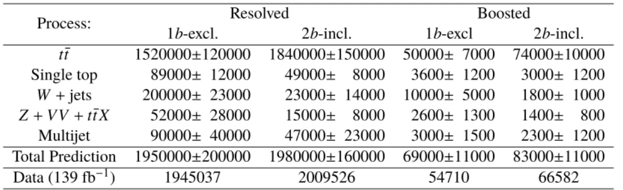
The event yields after the event selection can be found in Table 1.
Process: Resolved Boosted
1
b-excl. 2
b-incl. 1
b-excl 2
b-incl.
t¯t
1520000
±120000 1840000
±150000 50000
±7000 74000
±10000 Single top 89000
±12000 49000
±8000 3600
±1200 3000
±1200
W+jets 200000
±23000 23000
±14000 10000
±5000 1800
±1000
Z+V V+tt X¯ 52000
±28000 15000
±8000 2600
±1300 1400
±800 Multijet 90000
±40000 47000
±23000 3000
±1500 2300
±1200 Total Prediction 1950000
±200000 1980000
±160000 69000
±11000 83000
±11000
Data (139 fb
−1) 1945037 2009526 54710 66582
Table 1: Event yields split by topology (resolved, boosted) and b-tag multiplicity (1-excl., 2-incl.). Total pre- marginalisation uncertainty is shown.
The measurement of
AC, which is inferred from
∆|y|following Equation 1, is performed using a fit that maximises the extended likelihood of Equation 5. A combination of four channels based on the
b-jet multiplicity and the event topology (resolved or boosted) is employed. The
∆|y|distribution is split into four bins in all channels and in each differential bin of all differential measurements. Furthermore, since many BSM theories predict enhancement of the asymmetry at large
mtt¯and
βz,t¯tthe differential bins have been chosen based on a compromise between data statistics and event migration due to bad reconstruction.
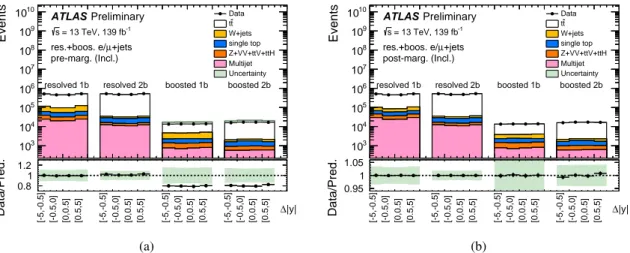
A normalisation difference between the data and the predictions on the order of 20% is observed in the boosted channel and can be seen on Figures 1 – 3. This overestimation of the MC predictions at large values of top
pT(>300 GeV), is confirmed by differential cross-sections measurements [127]. In order to compensate for this known mismodeling, an additional free normalisation parameter
Kboosteddescribed by a uniform prior in the range 0-2, is added in the boosted channel. The posterior probability density is:
p T|{D1· · ·DNch} = Z Nch
Y
i=1
L(Di|Ri(T,Kboosted
;
θs),Bi(θs,θb)) N(θs)N(θb)π(T) π(Kboosted)d
θsd
θb,(6)
where
B = B(θs,θb)is the total background prediction, the probability densities
πare uniform priors and
Ris the reconstructed signal prediction. Two categories of nuisance parameters are considered: the normalisation of the background processes (
θb), and the uncertainties associated with object identification, reconstruction and calibrations (
θs). The latter uncertainties are referred to as detector systematic uncertainties, and affect both the reconstructed distribution of the
t¯tsignal and the total background prediction. The additonal boosted
tt¯ normalisation factors are found to be
∼0
.8 with a relative uncertainty between 7 and 15% depending on the measurement.
A Bootstrap [128] method is applied in order to estimate the effect on the systematic uncertainties of limited MC statistics in the alternative samples. Only systematic variations which are found to be significant compared to their statistical precision are kept. When systematic effects are found not to be significant, the respective uncertainty is set to 0.
In addition, a pruning procedure is implemented in order to remove the smallest systematic uncertainties
and to simplify the marginalisation procedure. Since the
ACvalue is affected more by the shape effects of
the systematic uncertainties than by the normalisation effects, different pruning criteria are used to ignore the shape or normalisation effect of each systematic uncertainty.
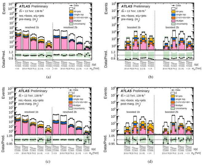
As shown on Figures 1 – 3, the marginalisation procedure reduces the total uncertainty significantly and improves the agreement between the data and the predictions.
103
104
105
106
107
108
109
1010
Events
resolved 1b resolved 2b boosted 1b boosted 2b
Data t t W+jets single top Z+VV+ttV+ttH Multijet Uncertainty
ATLAS Preliminary = 13 TeV, 139 fb-1
s
+jets µ res.+boos. e/
pre-marg. (Incl.)
0.8 1 1.2
Data/Pred. [-5,-0.5] [-0.5,0] [0,0.5] [0.5,5] [-5,-0.5] [-0.5,0] [0,0.5] [0.5,5] [-5,-0.5] [-0.5,0] [0,0.5] [0.5,5] [-5,-0.5] [-0.5,0] [0,0.5] [0.5,5]
∆|y|
(a)
103
104
105
106
107
108
109
1010
Events
resolved 1b resolved 2b boosted 1b boosted 2b
Data t t W+jets single top Z+VV+ttV+ttH Multijet Uncertainty
ATLAS Preliminary = 13 TeV, 139 fb-1
s
+jets µ res.+boos. e/
post-marg. (Incl.)
0.95 1 1.05
Data/Pred. [-5,-0.5] [-0.5,0] [0,0.5] [0.5,5] [-5,-0.5] [-0.5,0] [0,0.5] [0.5,5] [-5,-0.5] [-0.5,0] [0,0.5] [0.5,5] [-5,-0.5] [-0.5,0] [0,0.5] [0.5,5]
∆|y|
(b)
Figure 1: Comparison between the data and the prediction for bins used in the inclusiveACmeasurements in the lepton+jets channel. This comparison is shown before (left) and after (right) marginalisation within FBU. The bottom panels show the ratio of data to the predictions. The light green bands correspond to the total uncertainty of the prediction.
In order to determine the relative impact of each systematic uncertainty, pseudo-datsets are produced by shifting each systematics individually. These distributions are unfolded, and the difference between the resulting
ACvalues and the nominal unfolded
ACvalue is used to rank each systematic’s impact.
The results of the unfolded data are summarised in Table 2. The ranking of the leading systematic
uncertainties and the posterior probability distribution of
ACfor the inclusive measurement are shown in
Fig. 4.
103
104
105
106
107
108
Events
resolved 1b resolved 2b
Data t t W+jets single top Z+VV+ttV+ttH Multijet Uncertainty
ATLAS Preliminary = 13 TeV, 139 fb-1
s
+jets µ res.+boos. e/
)
t
βz,t
pre-marg. (
0.8 1 1.2
Data/Pred.
[0.0,0.3] [0.3,0.6] [0.6,0.8] [0.8,1.0] [0.0,0.3] [0.3,0.6] [0.6,0.8] [0.8,1.0]
∆|y|
t z,t β
[-5,-0.3] [-0.3,0] [0,0.3] [0.3,5] [-5,-0.3] [-0.3,0] [0,0.3] [0.3,5] [-5,-0.5] [-0.5,0] [0,0.5] [0.5,5] [-5,-0.7] [-0.7,0] [0,0.7] [0.7,5] [-5,-0.3] [-0.3,0] [0,0.3] [0.3,5] [-5,-0.3] [-0.3,0] [0,0.3] [0.3,5] [-5,-0.5] [-0.5,0] [0,0.5] [0.5,5] [-5,-0.7] [-0.7,0] [0,0.7] [0.7,5]
(a)
102
103
104
105
106
107
Events
boosted 1b boosted 2b
Data t t W+jets single top Z+VV+ttV+ttH Multijet Uncertainty
ATLAS Preliminary = 13 TeV, 139 fb-1
s
+jets µ res.+boos. e/
)
t
βz,t
pre-marg. (
0.8 1 1.2
Data/Pred.
[0.0,0.3] [0.3,0.6] [0.6,0.8] [0.8,1.0] [0.0,0.3] [0.3,0.6] [0.6,0.8] [0.8,1.0]
∆|y|
t z,t β
[-5,-0.3] [-0.3,0] [0,0.3] [0.3,5] [-5,-0.3] [-0.3,0] [0,0.3] [0.3,5] [-5,-0.5] [-0.5,0] [0,0.5] [0.5,5] [-5,-0.7] [-0.7,0] [0,0.7] [0.7,5] [-5,-0.3] [-0.3,0] [0,0.3] [0.3,5] [-5,-0.3] [-0.3,0] [0,0.3] [0.3,5] [-5,-0.5] [-0.5,0] [0,0.5] [0.5,5] [-5,-0.7] [-0.7,0] [0,0.7] [0.7,5]
(b)
103
104
105
106
107
108
Events
resolved 1b resolved 2b
Data t t W+jets single top Z+VV+ttV+ttH Multijet Uncertainty
ATLAS Preliminary = 13 TeV, 139 fb-1
s
+jets µ res.+boos. e/
t) βz,t
post-marg. (
0.95 1 1.05
Data/Pred. [0.0,0.3] [0.3,0.6] [0.6,0.8] [0.8,1.0] [0.0,0.3] [0.3,0.6] [0.6,0.8] [0.8,1.0] |y|∆
t z,t β
[-5,-0.3] [-0.3,0] [0,0.3] [0.3,5] [-5,-0.3] [-0.3,0] [0,0.3] [0.3,5] [-5,-0.5] [-0.5,0] [0,0.5] [0.5,5] [-5,-0.7] [-0.7,0] [0,0.7] [0.7,5] [-5,-0.3] [-0.3,0] [0,0.3] [0.3,5] [-5,-0.3] [-0.3,0] [0,0.3] [0.3,5] [-5,-0.5] [-0.5,0] [0,0.5] [0.5,5] [-5,-0.7] [-0.7,0] [0,0.7] [0.7,5]
(c)
102
103
104
105
106
107
Events
boosted 1b boosted 2b
Data t t W+jets single top Z+VV+ttV+ttH Multijet Uncertainty
ATLAS Preliminary = 13 TeV, 139 fb-1
s
+jets µ res.+boos. e/
t) βz,t
post-marg. (
0.95 1 1.05
Data/Pred. [0.0,0.3] [0.3,0.6] [0.6,0.8] [0.8,1.0] [0.0,0.3] [0.3,0.6] [0.6,0.8] [0.8,1.0] |y|∆
t z,t β
[-5,-0.3] [-0.3,0] [0,0.3] [0.3,5] [-5,-0.3] [-0.3,0] [0,0.3] [0.3,5] [-5,-0.5] [-0.5,0] [0,0.5] [0.5,5] [-5,-0.7] [-0.7,0] [0,0.7] [0.7,5] [-5,-0.3] [-0.3,0] [0,0.3] [0.3,5] [-5,-0.3] [-0.3,0] [0,0.3] [0.3,5] [-5,-0.5] [-0.5,0] [0,0.5] [0.5,5] [-5,-0.7] [-0.7,0] [0,0.7] [0.7,5]
(d)
Figure 2: Comparison between the data and the prediction for bins used in the βz,tt¯differentialACmeasurements in the lepton+jets channel. This comparison is shown before (upper) and after (lower) marginalisation within FBU for resolved (left) and boosted (right) topology. The bottom panels show the ratio of data to the prediction. The light green bands correspond to the total uncertainty of the prediction.