ATLAS NOTE ATLAS-CONF-2016-087

A TLAS-CONF-2016-087

ATLAS NOTE

ATLAS-CONF-2016-087

5th August 2016

A search for new phenomena in events with missing transverse momentum and a Higgs boson decaying to two photons in a 13.3 fb ⁻¹ p p collision dataset at √

s = 13 TeV with the ATLAS detector

The ATLAS Collaboration

Abstract

A search for new phenomena in events with large missing transverse momentum and a Higgs boson decaying to two photons is presented. The search uses 13 . 3 fb

of proton-proton collision data collected at a centre-of-mass energy of 13 TeV with the ATLAS detector at the CERN Large Hadron Collider in 2015 and 2016. No excess over the background expectation is observed. Limits are set on the production rates of the following theoretical models:

two simplified models where the Standard Model–dark matter interaction is mediated by a new vector particle emitting a Higgs boson and decaying, either directly or through an intermediate state, into two invisible particles, and an effective theory model where a heavy scalar decays into a Higgs boson and a pair of dark matter candidates.

© 2016 CERN for the benefit of the ATLAS Collaboration.

Reproduction of this article or parts of it is allowed as specified in the CC-BY-4.0 license.

1 Introduction

The discovery of a boson in 2012 by the ATLAS [1] and CMS [2] collaborations, consistent with the Standard Model (SM) Higgs boson, has opened up new channels to search for new physics. In particular, events with a Higgs boson and missing transverse momentum ( E

T

) in the final state can be sensitive probes of scenarios involving dark matter (DM) candidates.

The ATLAS Collaboration has previously searched for such events at a centre-of-mass energy of

√ s = 8 TeV [3] and with 3 . 2 fb

of data at

√ s = 13 TeV [4]. This note expands the search in Ref. [4] by adding 10 . 1 fb

of data obtained at 13 TeV in 2016. The definitions of the four categories have been re-optimized for the machine conditions during the 2016 data-taking.

This note is organized as follows. Section 2 summarizes the theoretical benchmarks used for this search.

Section 3 gives a brief description of the ATLAS detector. Section 4 describes the dataset and the signal and background Monte Carlo (MC) simulation samples used. Section 5 explains the reconstruction and identification of objects, while Section 6 outlines the optimization of the event selection and categoriza- tion. Section 7 summarizes the signal and background modeling. Section 8 discusses the experimental and theoretical systematic uncertainties that affect the results. Section 9 presents the results and their interpretations, and Section 10 gives a summary.

2 Theoretical Models

The results of the search are interpreted in three theoretical models. In two simplified models, a massive vector mediator, Z

, emits a Higgs boson and subsequently decays into a pair of DM candidates. In an effective theory model, a heavy scalar decays into a Higgs boson and two DM candidates. The models are briefly described below.

2.1 Simplified models of dark matter production in association with a Higgs boson

Z

Z

¯ q q

¯ χ

χ h

Z

A

¯ q q

¯ χ

χ h

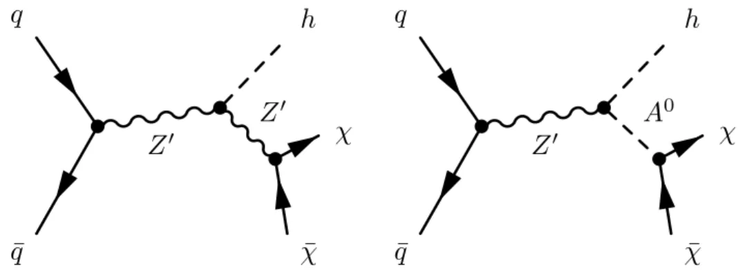
Figure 1: Collider production of dark matter in association with a Higgs boson, in two simplified models, each with a

mediator

In simplified models of DM production [5], the dark and the visible sectors can be coupled through a new

massive spin-0 or spin-1 mediator. Mono-Higgs signals, a Higgs boson in the final state accompanied by

DM particles escaping detection, are a prediction of many such scenarios because, in general, the mediator couples to the SM Higgs boson.

However, there is an important difference between searches for DM in mono-Higgs channels and other mono-X processes. In mono-X (jet, photon, W or Z) searches, the X is either emitted from a light quark as initial state radiation (ISR) through SM gauge interactions, or from a beyond the Standard Model (BSM) vertex coupling DM to the SM. In contrast, because the mass-dependent couplings suppress Higgs boson radiation from initial-state partons, typical mono-Higgs signals directly involve the Higgs boson in the BSM physics responsible for producing DM.

Two simplified models with vector mediators are used in this analysis. They both contain a Dirac fermion DM candidate and an additional vector boson, Z

, as the mediator. The choice of vector mediator is a common feature of many BSM theories, arising as a minimal extension to the gauge structure of the SM.

In scenarios where the DM couples to the SM only via the Z

, the associated U ( 1 )

symmetry ensures the stability of the DM particle [6]. These two models are among the models recommended by the LHC Dark Matter Forum [5], previously presented in Refs. [7, 8].

The first Z

mediated model used in this analysis is denoted as the Z

model [6]. The baryon number B is gauged under U (1)

, and an additional scalar referred to as a baryonic Higgs boson is introduced to spontaneously break this symmetry and generate the Z

mass. A vector mediator Z

produced via the s -channel radiates a Higgs boson and subsequently decays into two DM particles. A Feynman diagram for such a process is shown in Fig. 1 (left). The parameters of the Z

model are:

1. the coupling of Z

to DM particles, g

; 2. the coupling of Z

to quarks, g

;

3. the coupling of Z

to the SM Higgs boson, g

: this a dimensional parameter, with dimension of mass;

4. the mixing angle between the baryonic Higgs boson and the SM Higgs boson, sin θ ; 5. the mass of Z

, m

;

6. the mass of the DM particle, m

.

A second simplified model, referred to as the Z

-2HDM model [9], is also considered in the analysis.

This model contains a intermediate heavy pseudoscalar A

decaying to a pair of DM particles together with a vector mediator Z

. It has different kinematic distributions than the Z

model due to the on-shell production of Z

, which results in heavy Z

masses and therefore a harder E

T

spectrum. Figure 1(right) shows the related DM production process. The vector Z

is produced resonantly and decays into a Higgs boson and an intermediate heavy pseudoscalar A

, which in turn decays into two DM particles.

The motivation for generating DM from the decay of a pseudoscalar is that DM coupling to a vector is generically constrained by other signal channels and by direct detection searches. The Z

-2HDM model can satisfy electroweak precision tests and constraints from dijet resonance searches, while giving a potentially observable Higgs boson plus E

T

signal. The parameters of the Z

-2HDM model are:

1. the pseudoscalar mass, m

, 2. the mass of the DM particle, m

; 3. the mass of the Z

, m

;

4. the ratio of the two Higgs doublet vacuum expectation values, tan β ( ≡ v

/v

);

5. the coupling constant between the Z

, Higgs boson and pseudoscalar fields, g

. 2.2 Heavy scalar model

t t t g

g

H H

h

Figure 2: Production of a heavy scalar

via gluon fusion (left), and decay of the

into a Higgs boson (denoted as

) and a pair of dark matter candidates via an effective coupling (right).

The heavy scalar model [10] introduces a heavy scalar H 1 in the mass range of 2 m

< m

< 2 m

, which is produced primarily via gluon fusion (ggF) as shown in Fig. 2 (left). The upper bound on m

is to avoid large t t ¯ branching of the H . The DM mass m

is taken to be roughly half of the SM Higgs boson mass to ensure on shell decay of H → h χ χ , and suppress invisible decay modes of h . It also satisfies constraints from direct detection experiments [11]. The heavy scalar is allowed to decay into a Higgs boson and DM candidates, H → h χ χ , where χ is a DM candidate with spin-0, as shown in Fig. 2 (right). These interactions can be expressed by the Lagrangian:

L

= − 1

2 λ

H h χ χ − 1

4 λ

H H hh − 1

4 λ

hh χ χ − 1

4 λ

H H χ χ, (1) the first term of which contains an effective quartic coupling between h , H , and χ , relevant for this analysis. The larger branching ratio (BR) of the three-body decay of H to the SM Higgs boson and DM particles compared to two-body decays can be obtained by assuming that the DM candidates originate from the decay of some real scalar S . The masses m

and m

, as well as the branching ratios of the three decay modes of H , are free parameters of the model.

3 The ATLAS Detector

The ATLAS detector [12] is a multi-purpose particle physics detector with approximately forward- backward symmetric cylindrical geometry2. The inner tracking detector (ID) covers |η | < 2 . 5 and consists of a silicon pixel detector, a silicon micro-strip detector, and a transition radiation tracker (TRT) which allow a precise reconstruction of charged particle trajectories and of decay vertices of long lifetime particles. This is especially important for the present analysis in the case of photon conversion vertex reconstruction. The tracking system includes the newly installed innermost pixel layer, the insertable B-Layer (IBL) [13]. The ID is surrounded by a thin superconducting solenoid providing a 2 T axial magnetic field. A high-granularity lead/liquid-argon (LAr) sampling calorimeter measures the energy

1Throughout this note, a lowercasehrefers to the observed Higgs boson, while an uppercaseHrefers to the heavy scalar in this model.

2ATLAS uses a right-handed coordinate system with its origin at the nominal interaction point (IP) in the centre of the detector and thez-axis along the beam pipe. The x-axis points from the IP to the centre of the LHC ring, and the yaxis points upward. Cylindrical coordinates(r, φ)are used in the transverse plane,φbeing the azimuthal angle around the beam pipe.

The pseudorapidity is defined in terms of the polar angleθasη=−ln tan(θ/2).

and the position of electromagnetic showers in the central ( | η| < 1 . 475) and end-cap (1 . 375 < |η | < 3 . 2) regions. It includes the presampler (for |η| < 1 . 8) and three longitudinal sampling layers up to |η | < 2 . 5.

The first layer has a fine segmentation in the regions |η | < 1 . 4 and 1 . 5 < |η | < 2 . 4 to facilitate the separation of photons from neutral hadrons and to allow shower direction to be measured, while most of the energy is deposited in the second layer. LAr sampling calorimeters are also used to measure hadronic showers in the end-cap (1 . 5 < |η| < 3 . 2) and forward (3 . 1 < |η| < 4 . 9) regions, while an iron-scintillator/tile calorimeter measures hadronic showers in the central region ( | η| < 1 . 7). The muon spectrometer surrounds the calorimeters and consists of three large superconducting air-core toroid magnets, each with eight coils, a system of precision tracking chambers ( |η | < 2 . 7), and fast tracking chambers for triggering.

Events containing photon candidates are selected by a two-level trigger system. The first-level trigger is hardware based, while the second-level trigger is implemented in software [14].

4 Data and Simulated Samples

The analysis uses pp collision data with a bunch crossing interval of 25 ns, collected in 2015 and 2016 at

√ s = 13 TeV. Only events that were recorded in stable beam conditions when relevant detector components were functioning properly are considered. Events are collected using a diphoton trigger requiring two reconstructed photon candidates with transverse energies, E

, of at least 35 and 25 GeV for the leading and sub-leading photons, respectively. The data sample corresponds to an integrated luminosity of 13 . 3 fb

. Samples of signal events are generated using Madgraph [15] at leading order (LO) using the

NNPDF3.0LO [16] parton distribution function (PDF) set. Parton showering and hadronisation are simulated using the Pythia 8.186 [17] generator with the A14 tune [18], using the NNPDF2.3LO PDF set [19].

MC samples for the Z

model discussed in Section 2.1 are generated for a fixed DM particle mass of 1 GeV and for a range of mediator masses for which the LHC data are sensitive. The choice of this DM particle mass is motivated by the fact that DM searches at colliders are are most sensitive when the DM particle is light. The values of the coupling constants and mixing parameter are chosen following the recommendations of the LHC Dark Matter Forum [5]: g

= 1 . 0, g

= 1 / 3, g

= m

, sin θ = 0 . 3. For these values, the kinematic distributions predicted by the model are largely independent of the non-mass parameters, and thus the same values of these parameters are used to generate all samples.

Similarly, for the Z

-2HDM model discussed in Section 2.1, MC samples are generated for ranges of values of the mediator mass m

and pseudoscalar mass m

for which the search is sensitive. The DM mass m

is set to 100 GeVand the non-mass parameters, tan β = 1 . 0 and g

= 0 . 8, are also chosen as in Ref. [5] for all samples.

For the heavy scalar model described in Section 2.2, pp → H → h χ χ events are generated with m

in steps of 10 GeV in the interval 260 ≤ m

≤ 350 GeV, with an additional mass point at m

= 275 GeV, for m

= 50 and 60 GeV.

These simplified models and parameter sets were chosen to provide different yet equally plausible kinematic signatures of DM production in association with a Higgs boson. The dominant backgrounds to the h → γγ + E

T

process are SM h → γγ , non-resonant γγ , γ + jet, Wγ and Wγγ production. Additional processes

with final states containing photons, leptons or jets can contribute to the background since leptons and jets

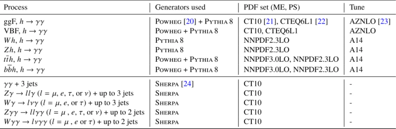
can be misidentified as photons. The SM Higgs boson processes considered in this analysis, along with details of the generators used, are shown in Table 1. The MC samples are used to model the background shape and evaluate uncertainties on the shape of the diphoton invariant mass ( m

) distribution and the normalisation of the m

shape of the SM Higgs boson. The normalisation of non-resonant backgrounds is directly obtained from data, as described in Section 7.

Table 1: Details of the generation of the SM Higgs boson and non resonant background processes considered in the analysis. The SM Higgs boson is generated with a mass of 125 GeV in all production modes. ggF and VBF denote gluon fusion and vector boson fusion respectively. The Sherpa generator uses the default tune. In the cases where different PDF sets are used for the matrix element (ME) generation and for the parton showering (PS), they are both listed. The non-resonant samples in the lower half are used only to optimize the event selection and ascertain systematic uncertainties but not used for deriving the limits since non-resonant backgrounds are directly fitted from the data.

Process Generators used PDF set (ME, PS) Tune

ggF,h→γγ Powheg [20] + Pythia 8 CT10 [21], CTEQ6L1 [22] AZNLO [23]

VBF,h→γγ Powheg + Pythia 8 CT10, CTEQ6L1 AZNLO

W h,h→γγ Pythia 8 NNPDF2.3LO A14

Z h,h→γγ Pythia 8 NNPDF2.3LO A14

tt h,h→γγ Powheg + Pythia 8 NNPDF3.0LO, NNPDF2.3LO A14

bbh,h→γγ Powheg + Pythia 8 NNPDF3.0LO, NNPDF2.3LO A14

γγ+ 3 jets Sherpa [24] CT10 -

Zγ→llγ(l=µ,e,τ, orν) + up to 3 jets Sherpa CT10 -

Wγ→lνγ(l=µ,e, orτ) + up to 3 jets Sherpa CT10 -

Zγγ→llγγ(l=µ,e,τ, orν) + up to 2 jets Sherpa CT10 -

Wγγ→lνγγ(l=µ,eorτ) + up to 2 jets Sherpa CT10 -

Detector effects are modelled by processing all MC samples through either a full simulation [25] or a fast simulation [26] of the ATLAS detector, based on Geant4 [27]. Corrections obtained from measurements in data are applied to the simulated events to account for small differences between data and simula- tion. The simulations include a realistic modelling of the multiple proton-proton collisions per bunch crossing (referred to as pile-up) observed in the data by overlaying additional interactions generated by Pythia 8 using the A2 [28] tune and the MSTW2008LO [29] PDF set. The simulated distribution of the average number of interactions per bunch crossing is reweighted to accurately reproduce the observed distribution.

5 Object Reconstruction and Identification

The reconstruction and identification of photons, leptons (electrons and muons), jets and E

T

are

summarized in this section.

5.1 Photons

Photons are reconstructed from clusters of energy deposits in the electromagnetic calorimeter measured

in projective towers. Clusters without matching tracks are classified as unconverted photon candidates.

A photon is considered as a converted photon candidate if it is matched to a pair of tracks that pass a TRT-hits requirement [30] and form a vertex in the ID which is consistent with originating from a massless particle, or if it is matched to a single track passing a TRT-hits requirement and having a first hit after the innermost layer of the pixel detector. The photon energy is calibrated using a multivariate regression technique trained with fully reconstructed MC samples. This energy is further corrected by applying in-situ calibration energy scale factors derived from Z → e

e

events and validated with Z → llγ events [31]. The simulation-based calibration procedure has been reoptimised for the 13 TeV data, and its performance was found to be compatible with that in Ref. [31] in the full pseudorapidity range used in the analysis. The photon resolution in simulation is corrected to match the resolution in the data.

This correction is derived simultaneously with the energy calibration factors using Z → e

e

events by adjusting the electron energy resolution such that the width of the reconstructed Z peak in simulation matches the width observed in data. The trajectory of the photon is reconstructed using the longitudinal segmentation of the calorimeters and a constraint from the average collision point of the proton beams.

For converted photons, the position of the conversion vertex is also used if tracks from the conversion have hits in the silicon detectors.

Identification requirements are applied to reduce the contamination of the photon sample from π

or other neutral hadrons decaying to two photons. The photon identification is based on the profile of the energy deposits in the first and second layers of the electromagnetic calorimeter. Photon candidates are required to deposit only a small fraction of their energy in the hadronic calorimeter and to have a lateral shower shape consistent with that expected from a single electromagnetic shower. The detailed shape of the shower in the high granularity first layer is used to discriminate single photons from hadronic jets in which a neutral meson carries most of the jet energy. The selection requirements are tuned separately for unconverted and converted photon candidates. The identification efficiency of unconverted (converted) photons range from 85% to 95% (90% to 98%) between 25 GeV and 200 GeV. Corrections are applied to the electromagnetic shower shape variables of simulated photons, to account for small differences observed between data and simulation. Candidate photons are required to have p

> 25 GeV and to satisfy the "loose" identification criteria defined in Ref. [32] and to be within |η| < 2 . 37, excluding the transition region of 1 . 37 < |η | < 1 . 52 between the barrel and end-cap calorimeters. Photons used in the event selection to form a Higgs boson candidate must also satisfy the "tight" identification criteria [32].

To further reject hadronic backgrounds, requirements on two complementary isolation variables are applied. The first variable is the sum of the transverse energies of positive-energy topological clusters [33]

deposited in the calorimeter within a cone of ∆R ≡ p

( ∆η)

+ ( ∆φ)

= 0 . 2 around each photon. The energy sum excludes the contribution of the photon cluster and an estimate of the energy deposited by the photon outside its associated cluster. To reduce the effects from the underlying event and pile-up, the isolation is further corrected using a method described in Ref. [34]. For each of the two different pseudorapidity regions |η | < 1 . 5 and 1 . 5 < |η | < 3 . 0, low-energy jets are used to compute an ambient energy density, which is then multiplied by the area of the isolation cone and subtracted from the isolation energy. To improve the efficiency of the isolation selection for events with large pile-up, the calorimeter isolation is complemented by a track-based isolation defined as the scalar sum of the transverse momenta of all tracks with p

> 1 GeV within a cone of size ∆R = 0 . 2 around each photon.

5.2 Leptons

Leptons ( e and µ ) are only used in the reconstruction of the missing transverse momentum (Section 5.4).

Hadronic decays of τ leptons are included in the jet contribution (Section 5.3) to the missing transverse

momentum.

Electrons are reconstructed from energy deposits measured in the electromagnetic (EM) calorimeter which are associated to ID tracks. They are required to satisfy |η| < 2 . 47, excluding the EM calorimeter transition region 1 . 37 < |η| < 1 . 52, have p

> 10 GeV and be identified using shower shape, track-cluster association and TRT criteria [35].

Muons are reconstructed from high-quality muon spectrometer segments associated to ID tracks. They are required to have p

> 10 GeV, |η | < 2 . 7 [36].

The muon and electron candidates are also required to be isolated with algorithms that are consistent with the photon isolation requirements. The significance of the transverse impact parameter, defined as the transverse impact parameter d

divided by its estimated uncertainty, σ

, of tracks with respect to the primary vertex is required to satisfy |d

|/σ

< 5.0 for electrons and | d

|/σ

< 3.0 for muons. The longitudinal impact parameter z

must satisfy | z

| sin θ < 0.5 mm for both electrons and muons. Electrons and muons close to photons are removed if the lepton is within ∆R < 0 . 4 of the photon.

5.3 Jets

Jets are reconstructed from the topological energy clusters in both the EM and hadronic calorimeters using the anti- k

algorithm [37] with a distance parameter of R = 0 . 4. Jets are required to have p

> 25 GeV and be in a region defined by |η | < 4 . 4. Quality criteria are applied to jets, and events with jets consistent with noise in the calorimeter or non-collision backgrounds are vetoed. To suppress pile-up jets found mainly at low p

, a jet vertex tagger [38] that uses tracking and vertexing information is applied on jets with p

< 60 GeV and |η | < 2 . 4 to select jets that have a high probability of originating at the diphoton production vertex (Section 6). Furthermore, if a jet is within ∆R < 0 . 4 of a photon or within ∆R < 0 . 2 of an electron, the jet is removed.

5.4 Missing Transverse Momentum

Missing transverse momentum is calculated as the negative vectorial sum of the transverse momenta of calibrated photons, electrons, muons and jets associated to the diphoton vertex. Energy depositions from the underlying event and other soft radiation are taken into account by constructing a soft term [39] from ID tracks associated to the same diphoton vertex [39, 40]. The soft term thus constructed is largely insensitive to pile-up.

6 Event Selection and Categorisation

At least two photon candidates with p

> 25 GeV are required to be in a fiducial region of the EM calorimeter defined by |η | < 2 . 37. Photon candidates in this fiducial region are ordered according to their E

and only the first two are considered: the leading and sub-leading photon candidates must have E

T

/m

> 0 . 35 and 0.25, respectively, where m

is the invariant mass of the two selected photons. The events are required to be within a window of 105 GeV < m

< 160 GeV around the Higgs boson mass.

These selections are following the previous ATLAS results on Higgs boson cross section measurement in

diphoton decay channel [41].

For the diphoton invariant mass, missing energy calculation and the track-based isolation computation, a precise knowledge of the position of the diphoton production vertex [42] is required. The diphoton production vertex is selected from the reconstructed collision vertices using a neural network algorithm.

For each vertex, the algorithm takes the following as input: the combined z -position of the intersections of the extrapolated photon trajectories with the beam axis; the sum of the squared transverse momenta P

p

T

and the scalar sum of the transverse momenta P

p

of the tracks associated with each reconstructed vertex;

the difference in azimuthal angle ∆φ between the direction defined by the vector sum of the track momenta with respect to each vertex and that of the diphoton system. The production vertex selection was studied with Z → e

e

events in data and in simulation by removing the electron tracks from the events. The MC simulation is found to accurately describe the efficiency measured in data. The integrated efficiency to locate the diphoton vertex within 0 . 3 mm of the production vertex for SM Higgs boson production via gluon fusion is 81%, and is slightly less for the signal samples.

In the Z

and Z

-2HDM models of DM production, the Higgs boson recoils against the DM pair, resulting in large E

T

in the event and large p

of the diphoton candidate, denoted as p

T

. By contrast, in the heavy scalar model, E

T

and p

T

can span a wide range, taking into account the different m

and m

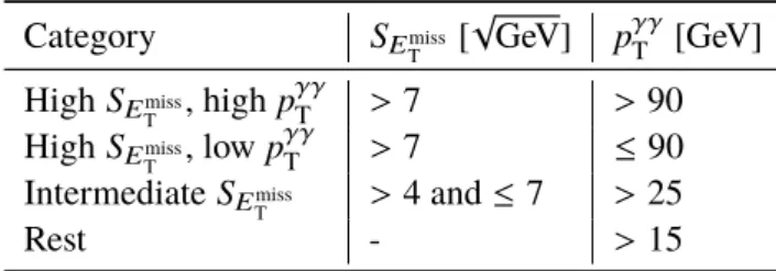
combinations. Consequently, dividing the events into multiple categories covers the sensitive regions of these different signal models. The events in the m

window are divided into four categories, as shown in Table 2, based on E

T

significance and p

T

, where E

T

significance is defined as the S

T

= E

T

/ √ P

E

. The sum in the denominator is the total transverse energy deposited in the calorimeters in the event 3.

The definition of the categories was adapted from the ATLAS result containing an analysis of Higgs boson decaying to diphoton pairs, produced in association with a Z-boson decaying into a neutrino pair [43], which has a similar final state. While the best sensitivity to the vector-mediator models lays almost completely in high S

T

categories, the lower S

T

categories have significant sensitivity to the heavy scalar model. Consequently, the intermediate and rest category definitions were optimized to improve the sensitivity to this model. The category with high S

T

and p

T

has by far the largest signal-to-background ratio for Z

and Z

-2HDM while for the heavy scalar model, the intermediate category contributes a lot to the sensitivity. Consequently, for the heavy scalar model, the results are extracted from a simultaneous likelihood fit over all four categories while the Z

and Z

-2HDM analysis only uses the category with high S

T

and p

T

to draw limits.

The significant increase of pile-up in 2016 resulted in a slight degradation of E

T

performance and led to the use of S

T

variable which is more resilient to pile-up and allows 2015 and 2016 data to be treated as a single dataset. This change was also motivated by the fact that the S

T

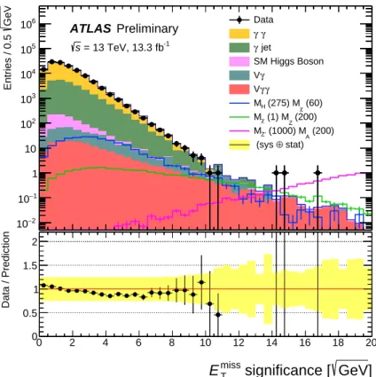
variable brings more sensitivity to the analysis. In Fig. 3, data and MC distributions for S

T

are compared inclusively. The bottom ratio plot shows as a yellow band the statistical uncertainties from MC samples added in quadrature with the systematic uncertainties. The same high-statistics MC γγ sample is also reweighted to describe the γ -jet contribution using a data driven measurement of γ -jet/ γγ lineshape as a function of the diphoton invariant mass. A data driven sample composition measurement, accounting for 78% γγ and 21% γ -jet is then used to build up the total γγ + γ -jet MC prediction. It has been checked that the agreement between MC and data is good within uncertainties in each specific category and the full difference between data and simulated samples has been taken as an additional systematic uncertainty on the SM Higgs boson

3The total transverse energy is calculated from the scalar sum of the transverse momenta of the calibrated hard objects and of thep_Tof the hard muons used in theE^miss

T calculation described in Section5, as well as energy deposits in the calorimeters not associated with any of the hard objects.

background. This non-resonant background shape from MC is also used to assess the spurious signal systematics as described in section 7.2.

] GeV significance [

miss

ET

GeVEntries / 0.5

−2

10

−1

10 1 10 102

103

104

105

106 ATLAS Preliminary = 13 TeV, 13.3 fb-1

s

Data γ γ γ jet

SM Higgs Boson γ

V γ γ V

(60) (275) Mχ

MH

(200) (1) MZ

Mχ

(200) (1000) MA

MZ'

stat)

⊕ (sys

] GeV significance [

miss

E

0 2 4 6 8 10 12 14 16 18 20

Data / Prediction

0 0.5 1 1.5 2

Figure 3: Inclusive

T

distribution in the full dataset compared to Monte Carlo shape prediction. The

sample shape is reweighted to the

T

distribution in the data. The

-jet shape is obtained from a reweighting of the

sample using a data driven measurement of

-jet/

ratio as a function of the diphoton mass. Finally, The

and

-jet are scaled to the data driven fraction, accounting for 78%, 21% of the total, respectively. The stack of background contributions is normalized to the data. A typical example of each signal model is shown. In the bottom ratio plot, the yellow band shows the statistical uncertainties from MC samples added in quadrature with the systematic uncertainties. The full difference between MC and data distribution shapes is taken into account when evaluating systematics on the limits set on the models investigated. In the statistical analysis, the non-resonant backgrounds are fitted from data and the MC samples of these backgrounds are not used.

7 Signal and Background Parameterisation

The signal is extracted by fitting an analytic function to the diphoton invariant mass distribution in each

category. The function describes the background and signal contributions. The full fit model includes the

signal, the SM Higgs boson background and the non-resonant backgrounds.

Table 2: Optimised criteria used in the categorisation. A ‘-’ denotes no requirement on that observable in that category, apart from the selections applied in Section

other categories. The

T >

15 GeV requirement in the ‘Rest’ category is motivated by the fact that the contribution from the SM Higgs boson produced via gluon fusion is very large at low values of

T

.

Category S

T

[

√

GeV] p

T

[GeV]

High S

T

, high p

T

> 7 > 90

High S

T

, low p

T

> 7 ≤ 90

Intermediate S

T

> 4 and ≤ 7 > 25

Rest - > 15

7.1 Modeling of Signals and SM Higgs Boson Background

For modeling the signal and the background from the SM Higgs boson, a double-sided Crystal Ball function4 is used, with parameters fit to the diphoton mass distribution of the relevant signal or the SM Higgs boson samples. The generated samples use a Higgs boson mass of 125 GeV. MC studies have shown that the shapes of the reconstructed m

spectra of the SM Higgs boson and the BSM signal samples agree with each other. Both the signal and the SM Higgs boson background are modeled using the relevant MC sample, separately in each of the four categories.

7.2 Modeling of Non-Resonant Background

The non-resonant background contribution is evaluated from data by fitting an analytic function to the m

distribution [44]. The form of the function is chosen by performing a test using templates built from background MC samples for non-resonant processes. The m

distributions from these samples are fitted in the range of 105 GeV < m

< 160 GeV with a signal plus a background model. Since no signal is present in these background-only samples, the resulting number of signal events from the fit, N

, can be taken as a measure of the bias in a particular background model. Such a bias is considered acceptable if N

is smaller than 10% of the expected signal rate of SM Higgs boson or smaller than 20% of the statistical uncertainty on the number of background events in the fitted signal peak in the mass range.

The largest N

in the mass range is taken as a systematic uncertainty on the background model. This procedure is referred to as a spurious signal test.

The spurious signal test is performed in the intermediate and the rest categories, which have sufficient numbers of events to enable such a test. An exponential of a second order polynomial is found to fulfill the requirements, and is used to model the background in these two categories. The systematic uncertainty corresponding to this function is 3% of the gluon-fusion produced Higgs boson contribution in the intermediate category and 13% of the same background in the rest category. Owing to the small number of events in the high S

T

categories, a spurious signal test is not feasible, and a simple exponential function is used to model the non-resonant background.

4A double-sided Crystal Ball function is composed of a Gaussian distribution at the core, with two power law distributions describing the lower and upper tails.

8 Systematic Uncertainties

Uncertainties from both experimental and theoretical sources affect the MC samples that are used in deriving the results of the analysis, i.e., the SM Higgs boson contribution and the signal samples. The major sources of uncertainties are briefly discussed in this section.

8.1 Experimental Uncertainties

Luminosity: The preliminary uncertainty on the combined 2015+2016 integrated luminosity is 2.9%. It is derived, following a methodology similar to that detailed in Refs. [45] and [46], from a preliminary calibration of the luminosity scale using x -y beam-separation scans performed in August 2015 and May 2016.

Trigger efficiency: The efficiency of the diphoton trigger used to select events is evaluated in MC using a trigger matching technique and in data using a bootstrap method [14]. The trigger efficiency for events in the diphoton invariant mass window of 105 GeV < m

< 160 GeV is found to be 99 . 44

(stat) ± 0 . 4 (syst) %.

Vertex selection efficiency: The uncertainty of the efficiency of this selection is found to be < 0 . 01%

from simulation.

Photon energy scale and resolution: The systematic uncertainties due to photon energy scale and res- olution have been taken mostly from Run-1 results [31], with minor updates in case of data driven corrections using the Run-2 data. The uncertainty on energy scale is less than 1% in the p

range of the photons used in this analysis, and less than 2% for the resolution.

Photon identification and isolation efficiency: In Run-1, the calorimeter shower shapes in MC were modified such that the photon identification efficiency measured in MC closely matched that meas- ured in data [32]. Similarly, the isolation momenta of ID tracks and the calorimeter isolation energy of photons in MC were shifted to match the photon isolation efficiency in MC to that measured in data [41]. The shifts used in Run-1 also describe the data well in Run-2. Uncertainties on the data/MC correction factors for photon identification and isolation efficiencies are evaluated as the difference between the correction factors with the shifts applied and not applied. The resulting uncertainty on the photon identification efficiency is ± 4 . 0%, while that on the photon isolation efficiency is ± 2 . 8%.

Migration uncertainty due to E

T

reconstruction: Migration of events among categories occurs ow- ing to changes in object energies/momenta, due mostly to misreconstruction of jets and E

T

. Although no direct jet selection is used in the analysis, the jet energy scale and resolution impact the calculation of E

T

. The impact of the uncertainties on jet energy scale, resolution and jet vertex fraction is estimated by varying each of these quantities by the amount of each component of the uncertainties independently of the other components, and recalculating E

T

for each variation. In addition, there are uncertainties on the scale and resolution of the E

T

soft term, evaluated on 2016 data using methods described in Ref. [39]. There are 20 uncorrelated uncertainties corresponding to jet energy scale and resolution, and 3 uncorrelated uncertainties corresponding to the E

T

soft term. The largest impact of these uncertainties on the event yield for the SM Higgs boson production is about 15% in the intermediate category, and about 10% in the high E

T

categories. For the

signal samples, the numbers are at most a few percent in any category. The uncertainties are smaller than 1% in the rest category.

Pile-up reweighting: The weights used to reweight the distribution of the average number of interactions per bunch crossing in simulation to the observed distribution (Section 4) are measured with an uncertainty. This uncertainty is taken into account by propagating it through the event selection, and results in a ± 1 . 0% uncertainty on the event yield of the signal and SM Higgs boson samples.

Mismodelling uncertainty of the S

T

: For SM gluon fusion Higgs boson production, the S

T

term

is not well modelled in simulation, hence a systematic uncertainty is derived by comparing the difference between data sidebands and background model. The systematic uncertainty is 25% for the High S

T

, high p

T

and 60% for High S

T

, low p

T

categories, with negligible effect overall since the effect is dominantly in the gluon-gluon fusion channel.

8.2 Theoretical Uncertainties

Scale uncertainty: The predicted cross sections of the SM Higgs boson and signal processes are affected by uncertainties due to missing higher-order terms in perturbative QCD. These uncertainties are estimated by varying the factorisation and renormalisation scales up and down from their nominal values by a factor of two, recalculating the cross section in each case, and taking the largest deviation from the nominal cross section as the uncertainty. In the case of the SM Higgs boson, the uncertainties are taken from Ref. [47]. In addition to an uncertainty on the inclusive cross section, the fact that a selection is made on the Higgs boson p

introduces an uncertainty on the SM Higgs boson production via gluon fusion. This uncertainty is evaluated as a function of the selection on the Higgs boson p

using the HRes2.3 [48] program5. The uncertainties are determined for a range of values of the Higgs boson p

selection by varying the factorisation and renormalisation scales up and down from their nominal values by a factor of two. The resulting uncertainty ranges from about 9% to about 20% for Higgs boson p

selection from 5 GeV to 120 GeV.

PDF uncertainty: For the SM Higgs boson samples, the PDF uncertainties are taken as in Ref. [47].

For the three signal processes, the PDF uncertainty is evaluated using the recommendations of PDF4LHC [49]. Both intra-PDF and inter-PDF uncertainties are extracted. Intra-PDF uncertainties are obtained by varying the parameters of the NNPDF3.0LO PDF set, while inter-PDF uncertainties are evaluated using alternative PDF sets. The final inter-PDF uncertainty is the maximum deviation among all the variations from the central value obtained using the NNPDF3.0LO PDF set.

Other theoretical uncertainties: The h → γγ branching ratio uncertainty is 4.9%, taken from Ref. [47].

The effect of multi-parton interactions (MPI) was evaluated by switching them on and off in Pythia 8 in the production of the gluon-fusion produced Higgs boson sample. The resulting uncertainty on the number of events in this sample is 50% in the high S

T

, low p

T

category.

A summary of the experimental and theoretical uncertainties is given in Table 3 in terms of the fractional impact on the number of events from SM Higgs boson production processes.

5HRes2.3 performs an analytical resummation of the ggF process and yields a cross section accurate up to NNLL+NNLO (next-to-next-to leading log and next-to-next-to leading order) in QCD.

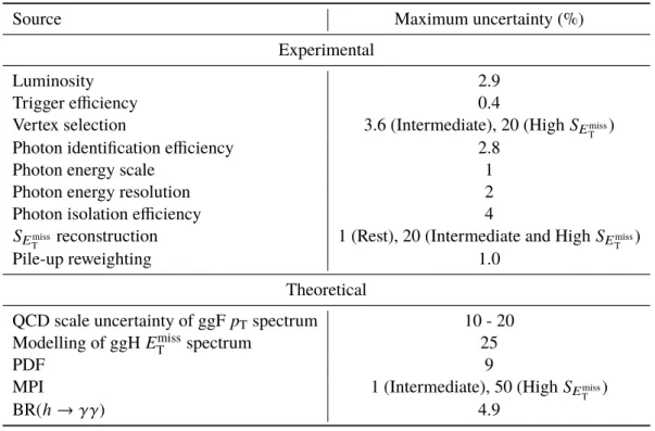
Table 3: Breakdown of the dominant systematic uncertainties on the yield of the SM Higgs boson processes estimated using SM Higgs boson MC. All production modes of the SM Higgs boson are considered together. Representative values for the impact on the four analysis categories are shown, unless a given source has very different impacts on different categories, in which case the largest and the smallest impacts are shown separately.

Source Maximum uncertainty (%)

Experimental

Luminosity 2.9

Trigger efficiency 0.4

Vertex selection 3.6 (Intermediate), 20 (High S

T

)

Photon identification efficiency 2.8

Photon energy scale 1

Photon energy resolution 2

Photon isolation efficiency 4

S

T

reconstruction 1 (Rest), 20 (Intermediate and High S

)

Pile-up reweighting 1.0

Theoretical

QCD scale uncertainty of ggF p

spectrum 10 - 20 Modelling of ggH E

T

spectrum 25

PDF 9

MPI 1 (Intermediate), 50 (High S

T

)

BR( h → γγ ) 4.9

9 Results

The event yields in data, signal and backgrounds within a window of 105 GeV < m

< 160 GeV in the four categories are shown in Table 4. The efficiencies for the three signal benchmarks in each category are also provided.

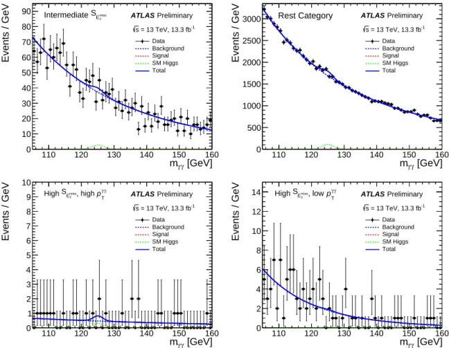
Figure 4 shows the m

distributions in the four categories as well as the fits for a simplified DM Z

model for illustration. No significant excess is observed in any category, so exclusion limits are set on the production cross sections of the theoretical models.

The statistical results of the analysis are derived from a likelihood fit, where the likelihood is a function of the observed events in each category, the expectations for the backgrounds and for the signal events in the respective models, the signal and background probability distribution functions, and the systematic uncertainties which are modeled as nuisance parameters. The fit is performed in the range 105 GeV <

m

< 160 GeV. Upper limits at 95% confidence level (CL) are calculated using a one-sided profile- likelihood ratio and the C L

formalism under the asymptotic approximation [50, 51].

Since high S

T

, high p

T

is the most sensitive category for signals from both Z

and Z

-2HDM models,

the results are only taken from this category for the vector mediator models. For the interpretation in the

Z

model, Fig. 5 shows 95% CL exclusion limits on σ(pp → h χ χ) ¯ × BR(h → γγ) as a function of the

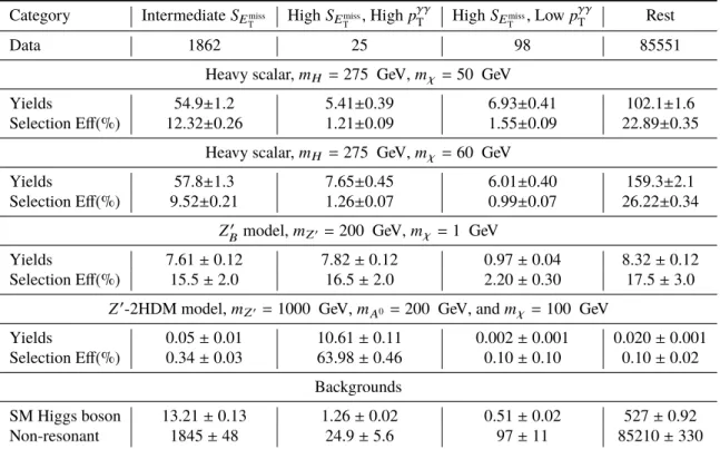
Table 4: Event yields in the range of 105 GeV

160 GeV for data, signal models, the SM Higgs boson background and non-Higgs boson backgrounds in each analysis category. The signal samples shown correspond to a heavy scalar model with

275 GeV and

60 GeV, a

model with

200 GeV and

1 GeV and a

-2HDM model with

1000 GeV,

200 GeV and

100 GeV. For the signal models, the selection efficiencies are also shown. The uncertainties on the signal yields consist of statistical and systematic uncertainties added in quadrature. The yields for non-resonant background are obtained from a fit to data in the side bands (excluding

in the range [120

130] GeV) while SM Higgs boson events are estimated from Monte Carlo.

This table corresponds to an integrated luminosity of 13

3

. Category Intermediate

T

High

T

, High

T

High

T

, Low

T

Rest

Data 1862 25 98 85551

Heavy scalar,

275 GeV,

50 GeV

Yields 54.9

1.2 5.41

0.39 6.93

0.41 102.1

1.6

Selection Eff(%) 12.32

0.26 1.21

0.09 1.55

0.09 22.89

0.35 Heavy scalar,

275 GeV,

60 GeV

Yields 57.8

1.3 7.65

0.45 6.01

0.40 159.3

2.1

Selection Eff(%) 9.52

0.21 1.26

0.07 0.99

0.07 26.22

0.34

model,

200 GeV,

1 GeV

Yields 7.61

0.12 7.82

0.12 0.97

0.04 8.32

0.12

Selection Eff(%) 15.5

2.0 16.5

2.0 2.20

0.30 17.5

3.0

Z⁰

-2HDM model,

1000 GeV,

200 GeV, and

100 GeV

Yields 0.05

0.01 10.61

0.11 0.002

0.001 0.020

0.001

Selection Eff(%) 0.34

0.03 63.98

0.46 0.10

0.10 0.10

0.02 Backgrounds

SM Higgs boson 13.21

0.13 1.26

0.02 0.51

0.02 527

0.92

Non-resonant 1845

48 24.9

5.6 97

11 85210

330

mediator mass m

for a DM mass of m

= 1 GeV. For m

= 10 GeV, σ( pp → h χ χ) ¯ × BR(h → γγ) is constrained to below 2.87 fb, while for m

= 2000 GeV, the upper limit is 0.87 fb.

For the interpretation in the Z

-2HDM model, Fig. 6 (left) shows 95% CL exclusion upper limits on σ( pp → h χ χ) ¯ × BR(h → γγ) as a function of the mediator mass m

A⁰

, for a DM mass of m

= 100 GeV, m

= 1000 GeVand sin θ = 0 . 3. For m

= 200 GeV, σ( pp → h χ χ) ¯ × BR( h → γγ) is constrained to be below 0.7 fb. Figure 6 (right) shows 95% CL exclusion upper limits on σ(pp → h χ χ) ¯ × BR( h → γγ) as a function of the mediator mass m

, for a DM particle mass of m

= 100 GeV and m

A⁰

= 200 GeV.

Figure 7 shows the observed 95% CL exclusion upper limits on pp → h χ χ ¯ cross section times branching ratio in the (m

, m

) plane for tan β = 1, g

= 0.8 and m

= 100 GeV.

In the heavy scalar interpretation, the 95% CL upper limits on the pp → H cross section times BR( H →

h χ χ → γγ χ χ ) as a function of m

for m

of 50 GeV and 60 GeV cases are shown in Fig. 8. The limits

are stronger at m

= 275 GeV, m

= 60 GeV than at other mass points because of statistical fluctuations

in the MC signal selection efficiency. For the scenario of DM mass at 50 GeV, the 95% CL upper limit is

18 . 2 fb for m

= 260 GeV, and 5 . 7 fb for m

= 350 GeV.

[GeV]

γ

mγ

110 120 130 140 150 160

Events / GeV

0 10 20 30 40 50 60 70 80

90 ATLAS Preliminary

= 13 TeV, 13.3 fb-1

s Data Background Signal SM Higgs Total

T

Emiss

Intermediate S

[GeV]

γ

mγ

110 120 130 140 150 160

Events / GeV

0 500 1000 1500 2000 2500

3000 ATLAS Preliminary

= 13 TeV, 13.3 fb-1

s Data Background Signal SM Higgs Total

Rest Category

[GeV]

γ

mγ

110 120 130 140 150 160

Events / GeV

0 1 2 3 4 5 6 7 8 9 10

Preliminary ATLAS

= 13 TeV, 13.3 fb-1

s Data Background Signal SM Higgs Total γ

γ

pT

, high

T

Emiss

High S

[GeV]

γ

mγ

110 120 130 140 150 160

Events / GeV

0 2 4 6 8 10 12

14 ATLAS Preliminary

= 13 TeV, 13.3 fb-1

s Data Background Signal SM Higgs Total γ

γ

pT

, low

T

Emiss

High S

Figure 4: Diphoton invariant mass distribution for data and the corresponding fitted signal and background in the four categories. The non-resonant background and the predicted SM Higgs boson contributions are shown. The fit result including signal, SM Higgs boson and non-resonant background are shown by the blue curve. The fit depicted constrains the signal contribution to be non-negative, and its best-fit value is zero, which is shown here. The fitted signal shown here is the

model with a DM particle mass of 1 GeV and

= 20 GeV.

10 Conclusion

Searches for new phenomena in diphoton events with different E

T

requirements are presented with 13 . 3 fb

of proton-proton collision data collected at the centre-of-mass energy of 13 TeV with the ATLAS detector at the LHC in 2015 and 2016.

No significant excess over the background expectation is observed. The results of the analysis are interpreted in the context of three theoretical models. For the simplified model of dark matter production involving a massive vector mediator Z

, a 95% CL upper limit of 3 fb is set on the cross-section times branching ratio of h to χ χ ¯ for a mediator mass of 50 GeV and a dark matter mass of 1 GeV. For the Z

-2HDM model, 95% CL exclusion limits on cross-section times branching ratio of h to χ χ ¯ are shown as a function of the pseudoscalar mass m

A⁰

and vector mediator mass m

. In the model involving heavy

scalar production, a 95% CL upper limit of 18 . 2 (23.9) fb is set on the product of the cross-section and

the branching fraction into the h → γγ final state with a DM particle of 50 (60) GeV. With respect to the

[GeV]

m

0 500 1000 1500 2000

) [fb] γγ → BR(h × ) χχ h → (pp σ 95% CL limit on

1 10 10

10

Observed Expected

σ

± 1 Expected

σ

± 2 Expected

Preliminary ATLAS

= 13 TeV, 13.3 fb-1

s

model , Z'B

χ χ γ) + γ

→ h(

pp

= 1 GeV = 1, mχ

gχ

= 1/3, gq

= 0.3, θ sin

Figure 5: Expected and observed 95% CL exclusion upper limits on the product of the cross section of

¯ and BR(

) in the

model corresponding to couplings of

= 1/3,

= 1 and sin

= 0.3. The limits are shown as a function of the mediator mass for a fixed DM particle mass of 1 GeV.

[GeV]

A0

m

200 300 400 500 600 700 800

) [fb]γγ→ BR(h ×) χχ h→(pp σ95% CL limit on

−1

10 1 10 102

Observed Expected

σ

± 1 Expected

σ

± 2 Expected

Preliminary ATLAS

= 13 TeV, 13.8 fb-1 s

, Z'-2HDM model χ

χ γ) + γ

→ h(

pp

= 1000 GeV mZ'

= 100 GeV, mχ

= 0.8, gZ' = 1.0, β tan

[GeV]

mZ'

400 600 800 1000 1200 1400

) [fb]γγ→ BR(h ×) χχ h→(pp σ95% CL limit on

−1

10 1 10 102

103

Observed Expected

σ

± 1 Expected

σ

± 2 Expected

Preliminary ATLAS

= 13 TeV, 13.3 fb-1 s

, Z'-2HDM model χ

χ γ) + γ

→ h(

pp

= 200 GeV A0

m = 100 GeV, mχ

= 0.8, gZ' = 1.0, β tan

Figure 6: (Left) Expected and observed 95% CL exclusion upper limits on the product of the cross section of

¯ and BR(

) in the

-2HDM model corresponding to couplings of tan

= 1,

= 0.8, and

m

=1000 GeV. The limits are shown as a function of the pseudoscalar A

mass for a fixed DM particle mass of

100 GeV. Also shown are the expected limits on

¯

for this model. (Right) Expected

and observed 95% CL exclusion upper limits on the product of the cross section of

¯ and BR(

) in

the

-2HDM model corresponding to couplings of tan

= 1,

= 0.8, m

=200 GeV. The limits are shown as a

function of

mass for a fixed DM particle mass of 100 GeV.

) [fb]γγ→ BR(h ×) χχ h→(pp σ95% CL limit on

0.6 0.8 1 1.2 1.4 1.6 1.8 2 2.2

[GeV]

m

400 600 800 1000 1200 1400

[GeV]

m

200 205 210 215 220 225 230

) [fb]γγ→ BR(h ×) χχ h→(pp σ95% CL limit on

0.6 0.8 1 1.2 1.4 1.6 1.8 2 2.2 Preliminary

ATLAS

= 13 TeV, 13.3 fb-1

s

, Z'-2HDM model χ

χ γ) + γ

→ h(

pp

= 100 GeV mχ

= 0.8, gZ

= 1.0, β tan

Figure 7: Observed 95% CL exclusion limits on the

¯

of

¯ in the (m

, m

) plane for tan

= 1,

= 0.8 and

= 100 GeV for the

-2HDM model.

[GeV]

mH

260 280 300 320 340 360

BR [fb]× H) →(ppσ95% CL Limit on 10

20 30 40 50 60 70 80 90

Observed 95% CL Expected 95% CL

σ

± 1 Expected

σ

± 2 Expected ATLAS Preliminary

γ γ

→ χ, h χ

→ h H

= 13 TeV, 13.3 fb-1

s = 50 GeV mχ

[GeV]

mH

260 280 300 320 340 360

BR [fb]× H) →(ppσ95% CL Limit on

20 40 60 80 100 120

Observed 95% CL Expected 95% CL

σ

± 1 Expected

σ

± 2 Expected ATLAS Preliminary

γ γ

→ χ, h χ

→ h H

= 13 TeV, 13.3 fb-1

s = 60 GeV mχ

Figure 8: Expected and observed 95% CL exclusion upper limits on the product of the cross section and BR(

,

) for the heavy scalar model, with a DM candidate mass of 50 GeV (left) and 60 GeV (right). The limits are shown as a function of the heavy scalar mass in the range between 260 GeV and 350 GeV for a DM candidate mass of 50 GeV (60 GeV).

last ATLAS public results, the present limits are improved by more than a factor of two due to the new

data and the improvements in the categorisation.

References

[1] ATLAS Collaboration, Observation of a new particle in the search for the Standard Model Higgs boson with the ATLAS detector at the LHC , Phys. Lett. B716 (2012) 1,

arXiv: 1207.7214 [hep-ex] . [2] CMS Collaboration,

Observation of a new boson at a mass of 125 GeV with the CMS experiment at the LHC , Phys. Lett. B716 (2012) 30, arXiv: 1207.7235 [hep-ex] .

[3] ATLAS Collaboration, Search for Dark Matter in Events with Missing Transverse Momentum and a Higgs Boson Decaying to Two Photons in pp Collisions at √

s = 8 TeV with the ATLAS Detector , Phys. Rev. Lett. 115 (2015) 131801, arXiv: 1506.01081 [hep-ex] .

[4] ATLAS Collaboration,

Search for new phenomena in events with missing transverse momentum and a Higgs boson decaying to two photons in p p collisions at √

s = 13 TeV with the ATLAS detector , ATLAS-CONF-2016-011, 2016, url: https://cds.cern.ch/record/2139812 .

[5] D. Abercrombie et al., Dark Matter Benchmark Models for Early LHC Run-2 Searches: Report of the ATLAS/CMS Dark Matter Forum , (2015), arXiv: 1507.00966 [hep-ex] .

[6] L. Carpenter et al., Mono-Higgs-boson: A new collider probe of dark matter , Phys. Rev. D89 (2014) 075017, arXiv: 1312.2592 [hep-ph] .

[7] J. Abdallah et al., Simplified Models for Dark Matter and Missing Energy Searches at the LHC , (2014), arXiv: 1409.2893 [hep-ph] .

[8] J. Abdallah et al., Simplified Models for Dark Matter Searches at the LHC , Phys. Dark Univ. 9-10 (2015) 8, arXiv: 1506.03116 [hep-ph] .

[9] A. Berlin, T. Lin and L.-T. Wang, Mono-Higgs Detection of Dark Matter at the LHC , JHEP 06 (2014) 078, arXiv: 1402.7074 [hep-ph] .

[10] M. Kumar et al., The impact of additional scalar bosons at the LHC , (2016), arXiv: 1603.01208 [hep-ph] .

[11] J. M. Cline et al., Update on scalar singlet dark matter ,

Phys. Rev. D88 (2013) 055025, [Erratum: Phys. Rev.D92,no.3,039906(2015)], arXiv: 1306.4710 [hep-ph] .

[12] ATLAS Collaboration, The ATLAS Experiment at the CERN Large Hadron Collider , JINST 3 (2008) S08003.

[13] ATLAS Collaboration, ATLAS Insertable B-Layer Technical Design Report , CERN-LHCC-2010-013, 2010, url: https://cds.cern.ch/record/1291633 . [14] ATLAS Collaboration, Performance of the ATLAS Trigger System in 2010 ,

Eur. Phys. J. C72 (2012) 1849, arXiv: 1110.1530 [hep-ex] .

[15] J. Alwall et al., MadGraph/MadEvent v4: The New Web Generation , JHEP 09 (2007) 028, arXiv: 0706.2334 [hep-ph] .

[16] R. D. Ball et al., Parton distributions for the LHC Run II , JHEP 04 (2015) 040, arXiv: 1410.8849 [hep-ph] .

[17] T. Sjostrand, S. Mrenna and P. Skands, A brief introduction to PYTHIA 8.1 ,

Comput. Phys. Commun. 178 (2008) 852, arXiv: 0710.3820 [hep-ph] .