ATLAS-CONF-2016-057 08August2016
ATLAS NOTE
ATLAS-CONF-2016-057
3rd August 2016
Search for massive supersymmetric particles in multi-jet final states produced in pp collisions at √
s = 13 TeV using the ATLAS detector at the LHC
The ATLAS Collaboration
Abstract
Results of a search for supersymmetric gluino pair productions with subsequent R-parity- violating decays to quarks are presented. This search uses 14.8 fb−1 of data collected by the ATLAS detector in proton-proton collisions with a center-of-mass energy of
√s = 13 TeV at the LHC. The analysis is performed using both a requirement on the number of jets and the number of jets tagged as containing ab-hadron as well as a topological observable formed from the scalar sum of large-radius jet masses in the event. No significant deviation is observed from the expected Standard Model backgrounds. For a model where the gluino decays through an intermediate neutralino which, in turn, decays to three quarks, gluino masses (mg˜) below 1000-1550 GeV are excluded depending on the neutralino mass. Gluinos decaying directly to three quarks are excluded formg˜<1080 GeV.
© 2016 CERN for the benefit of the ATLAS Collaboration.
Reproduction of this article or parts of it is allowed as specified in the CC-BY-4.0 license.
1 Introduction
Supersymmetry (SUSY) [1–6] is a theoretical extension of the Standard Model (SM) which fundamentally relates fermions and bosons. It is an alluring theoretical possibility given its potential to solve the naturalness problem [7,8].
This note presents a search forR-parity-violating (RPV) [9–14] supersymmetric gluino pair production with subsequent decays to quarks in events with many jets using 14.8 fb−1 ofppcollision data at
√s = 13 TeV collected by the ATLAS detector in 2015 and 2016. In supersymmetry, the RPV component of a generic super pontential can be written as [15,16]:
W6Rp = 12λi j kLiLjE¯k +λ0i j kLiQjD¯k + 12λ00i j kU¯iD¯jD¯k+κiLiH2, (1) where i,j,k = 1,2,3 are generation indices. The generation indices are sometimes omitted in the discussions that follow if the statement being made is not specific to any generation. The first three terms in Eq. (1) are often referred to as the trilinear couplings, whereas the last term is referred to as bilinear.
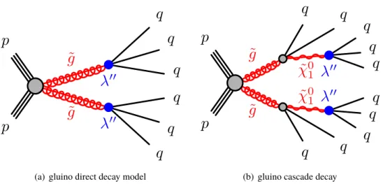
TheLi,Qi represent the lepton and quarkSU(2)Ldoublet superfields, whereasH2represents the Higgs superfield. The ¯Ej, ¯Dj, and ¯Ujare the charged lepton, down-type quark, and up-type quarkSU(2)Lsinglet superfields, respectively. The couplings for each term are given byλ,λ0, andλ00, andκis a dimensional mass parameter. In the benchmark models considered in this search, only the baryon-number-violating coupling λi j k00 is non-zero, in order to protect the proton from rapid decay. Because of the structure of Eq. (1), scenarios in which onlyλ00i j k ,0 are often referred to as UDD scenarios. The diagrams shown in Figure1represent the benchmark processes used in the optimization and design of the search presented in this note. In the gluino direct decay model (Figure1(a)), the gluino directly decays to three quarks via the RPV UDD couplingλ00, leading to six quarks in the final state of gluino pair production. In the gluino cascade decay model (Figure1(b)), the gluino decays to two quarks and a neutralino, which, in turn, decays to three quarks via the RPV UDD coupling λ00, resulting in ten quarks in the final state of gluino pair production. Events produced in these processes typically have a high multiplicity of reconstructed jets as well as complex event topology. In signal models considered in this search, the production of the gluino pair is assumed to be independent of the value ofλ00. All possibleλ00 flavor combinations given by the structure of Eq.1are assumed to proceed with equal probability, and decays of the gluino and neutralino are assumed to be prompt. Under this configuration, a significant portion of signal events contain at least one bottom or top quark. Other models of the RPV UDD scenario, such as the Minimum Flavor Violation model [17,18], also predict that the gluino decays preferably to final states with third generation quarks.
These theoretical arguments motivate the introduction ofb-tagging requirements to the search.
This analysis is an update to previous ATLAS searches for signals arising from RPV UDD scenarios [19, 20] performed with data taken during LHC Run-1. The search strategy follows closely the one implemented by the ATLAS Collaboration using LHC Run-1 data at
√s = 8 TeV in Ref. [20], which has excluded a gluino with mass up to 917 GeV in the gluino direct decay model, and a gluino with mass up to 1 TeV for a neutralino mass of 500 GeV in the gluino cascade decay model.
In a recent publication [21], the CMS collaboration also set a limit on the gluino mass up to 1.03 TeV in a RPV UDD scenario where the gluino exclusively decays to a final state of a top quark, a bottom quark and a strange quark, using
√s =8 TeVppcollision data.
˜ g
˜ g p
p
λ00
q q
q
λ00
q q q
(a) gluino direct decay model
˜ g
˜ g
˜ χ01
˜ χ01 p
p
q q
λ00 q
q q
q q
λ00 q
q q
(b) gluino cascade decay
Figure 1: Diagrams for the benchmark processes considered for this analysis. The black lines represent Standard Model particles, the red lines represent SUSY partners, the gray shaded circles represent effective vertices that include off-shell propagators (e.g. heavy squarks coupling to a ˜χ0
1neutralino and a quark), and the blue solid circles represent effective RPV vertices allowed by the baryon-number-violatingλ00couplings with off-shell propagators (e.g. heavy squarks coupling to two quarks).
2 ATLAS detector
The ATLAS detector [22] covers almost the whole solid angle around the collision point with layers of tracking detectors, calorimeters and muon chambers. For the measurements presented in this note, the calorimeters are of particular importance. The inner detector, immersed in a magnetic field provided by a solenoid, has full coverage inφand covers the pseudorapidity range|η| <2.51. It consists of a silicon pixel detector, a silicon microstrip detector and a transition radiation straw-tube tracker. The innermost pixel layer [23] was added between Run-1 and Run-2 of the LHC, around a new thinner (radius of 25 mm) beam pipe. In the pseudorapidity region|η| < 3.2, high granularity lead liquid-argon (LAr) electromagnetic (EM) sampling calorimeters are used. A steel-scintillator tile calorimeter provides hadronic calorimetry coverage over|η| < 1.7. The end-cap and forward regions, spanning 1.5 < |η| < 4.9, are instrumented with LAr calorimetry for both EM and hadronic measurements. The muon spectrometer surrounds these calorimeters, and comprises a system of precision tracking chambers and trigger detectors with three large toroids, each consisting of eight coils providing the magnetic field for the muon detectors. A two-level trigger system is used to select events [24]. The first-level trigger is implemented in hardware and uses a subset of the detector information. This is followed by the software-based High-Level Trigger, which can run offline reconstruction and calibration software, reducing the event rate to about 1 kHz.
1ATLAS uses a right-handed coordinate system with its origin at the nominal interaction point in the center of the detector and thez-axis along the beam direction. Thex-axis points toward the center of the LHC ring, and they-axis points upward.
Cylindrical coordinates(r, φ) are used in the transverse plane, φbeing the azimuthal angle around the beam pipe. The pseudorapidityηis defined in terms of the polar angleθbyη≡ −ln[tan(θ/2)].
3 Simulation samples
Signal samples are produced covering a wide range of gluino and neutralino masses. In the gluino direct decay model, the gluino mass (mg˜) is varied from 900 GeV to 1800 GeV. In the case of the cascade decays, for each gluino mass (1000 GeV to 1.9 TeV), separate samples are generated with multiple neutralino masses (m
χ˜0
1) ranging from 50 GeV to 1.65 TeV. In each case, m
χ˜0
1 < mg˜. Signal samples are generated at the leading order (LO) using the MadGraph5_aMC@NLO v2.3.3 event generator [25]
interfaced to Pythia 8.186 [26]. The A14 [27] tune is used together with the NNPDF2.3LO [28] parton distribution function (PDF) set. The EvtGen v1.2.0 program [29] is used to describe the properties of the b- andc- hadron decays in the signal samples and the background samples except those produced with Sherpa [30]. The signal production cross-sections are calculated at next-to-leading order (NLO) in the strong coupling constant, adding the resummation of soft gluon emission at next-to-leading-logarithmic accuracy (NLO+NLL) [31–35]. The nominal cross-section and its uncertainty are taken from Ref. [36].
Cross-sections are evaluated assuming masses of 450 TeV for the light-flavour squarks in case of gluino pair production. In the simulation, the total widths of gluino and neutralino are set to be 1 GeV, effectively making their decays prompt.
While a data-driven method is used to estimate the background, simulated events are used to establish, test and validate the methodology of the analysis. Therefore, simulation is not required to precisely describe the background, but it should be sufficiently similar that the strategy can be tested before applying it to data. Multi-jet events constitute the dominant background in the search region, with small contributions from top-quark pair-production (t¯t). Contributions fromγ+ jets,W+ jets,Z+ jets, single-top quark, and diboson background processes are negligible from simulation.
The multi-jet background is generated with Pythia 8.186 using the A14 tune and the NNPDF2.3LO parton distribution functions. Sherpa multi-jet samples are also generated and tested for the background estimation. Matrix elements are calculated with up to 3 partons at LO and merged with the Sherpa parton shower [37] using the ME+PS@LO prescription [38]. The CT10 PDF set [39] is used in conjunction with dedicated parton shower tuning developed by the Sherpa authors.
For the generation of fully hadronic decayingtt¯events, the Powheg-Box v2 [40] generator is used with the CT10 PDF set. The parton shower, fragmentation, and the underlying event are simulated using Pythia 6.428 [41] with the CTEQ6L1 PDF set [42] and the corresponding Perugia 2012 tune (P2012) [43].
The effect of additionalppinteractions per bunch crossing (“pile-up”) as a function of the instantaneous luminosity is taken into account by overlaying simulated minimum-bias events according to the observed distribution of the number of pile-up interactions in data. All Monte-Carlo (MC) simulated background samples are passed through a full GEANT4 [44] simulation of the ATLAS detector [45]. The signal samples are passed through a fast detector simulation based on a parameterization of the performance of the ATLAS electromagnetic and hadronic calorimeters [46] and on GEANT4 elsewhere.
4 Event selection
The data used here were recorded in 2015 and 2016, with the LHC operating at a center-of-mass energy of
√s =13 TeV. All detector elements are required to be fully operational. The integrated luminosity is measured to be 3.2 fb−1and 11.6 fb−1, for the 2015 data set and 2016 data set, respectively. The luminosity measurement was calibrated during dedicated beam-separation scans, using the same methodology as that
described in [47]. The uncertainty of this measurement is found to be 2.1% for 2015 data, and 3.7% for 2016 data. In this analysis, the 2015 and 2016 data sets are combined and treated as a single data set, corresponding to a total integrated luminosity of 14.8 fb−1.
The events used in this search are selected using a large-Rjet trigger, which requires at least one anti-kt jet [48] with a radius of 1.0 and apT >420 GeV.
Events are required to have a primary vertex with at least two associated tracks withpTabove 0.4 GeV.
The primary vertex assigned to the hard-scattering collision is the one with the highestP
trackp2
T, where the scalar sum of trackp2
Tis taken over all tracks associated with that vertex.
Since the signal process is characterised by the presence of many quarks, the analysis only considers jets in the events. Jets are reconstructed from three-dimensional topological clusters of energy deposits in the calorimeter calibrated at the EM scale [49], using the anti-kt algorithm with two different radius parameters of R = 1.0 and R = 0.4, hereafter referred to as large-R jets and small-R jets, respectively.
The four-momenta of the jets are calculated as the sum of the four-momenta of the clusters, which are assumed to be massless. For the large-Rjets, the original constituents are calibrated using the local cluster weighting algorithm [50] and reclustered using the longitudinally-invariantktalgorithm [51] with a radius parameter ofRsub−j et= 0.2, to form a collection of sub-jets. A sub-jet is discarded if it carries less than 5% of the pT of the original jet. The constituents in the remaining sub-jets are then used to recalculate the large-R jet four-momenta, and the jet energy and mass are further calibrated to particle level using correction factors derived from simulation [52]. The resulting “trimmed” [53] large-Rjets are required to havepT > 200 GeV and |η| < 2.0. The analysis selects events with at least three large-Rjets and requires thepT of leading large-Rjet to be greater than 440 GeV so that the trigger is fully efficient with respect to the analysis selection. Events with three large-R jets are used to derive jet mass templates. Events with higher large-Rjet multiplicity are used to validate background estimation performance and probe the existence of Beyond SM (BSM) signals. The small-R jets are corrected for pile-up contributions and are then calibrated to the particle level using simulation followed by a correction based on in-situ measurements [54].
The identification of jets containingb-hadrons is based on the small-Rjet with pT > 50 GeV and |η| <
2.5 and a multivariate tagging algorithm [55,56]. This algorithm is applied to a set of tracks with loose impact parameter constraints in a region of interest around each jet axis to enable the reconstruction of theb-hadron decay vertex. Theb-tagging requirements result in an efficiency of 70% for jets containing b-hadrons, as determined in a sample of simulatedt¯t events [56]. A small-Rjet passing the b-tagging requirement is considered as ab-jet. The events selected in the analysis are further divided to ab-tag sample where at least oneb-jet is present in the event, and ab-vetosample where nob-jet is present in the event. Events selected without ab-tagging requirement are referred to asinclusiveevents.
5 Analysis strategy
The analysis uses a topological observable, the total jet mass variable,MΣ
J, as the primary discriminating variable to separate signal and background. The observableMΣ
J [57–59] is defined as the scalar sum of
the masses of the four leading large-Rjets reconstructed with a radius parameterR=1.0,pT >200 GeV and|η| <2.0,
MΣ
J = X4
pT>200 GeV
|η|≤2.0
mjet. (2)
This observable was used for the first time in the
√s = 8 TeV search by the ATLAS Collaboration for events with many jets and missing transverse momentum [60] and provides significant sensitivity for very high-mass gluinos. It was also used in the search by the ATLAS Collaboration for RPV SUSY in events with many jets using the Run-1 LHC data [20]. Here, the four leading jets in the event are used, as they cover a significant portion of the central region of the calorimeter, and are very likely to capture most signal quarks.
Simulation studies show thatMΣ
J provides greater sensitivity than variables such asHTor the scalar sum of jetpT. The masses contain angular information about the events, whereas a variable like HT simply describes the energy (or transverse momentum) in the event. A largeMΣ
J implies not only high energy of the mult-jet system, but also rich angular structure. Previous studies with the Monte Carlo generators have demonstrated the power of theMΣ
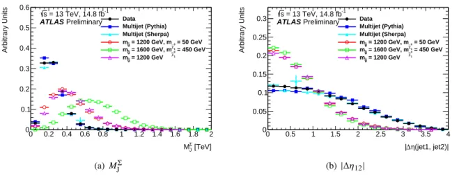
J variable in the high-multiplicity events that this analysis targets [57, 58]. Figure 2(a)presents examples of the discrimination that the MΣ
J observable provides between the background (represented here by Sherpa and Pythia 8.186 multi-jet MC simulation) and several signal samples, as well as the comparison of the data to the Monte Carlo multi-jet background.
Another discriminating variable that is independent ofMΣ
J is necessary in order to define suitable con- trol and validation regions where the background estimation can be studied and tested. The signal is characterized by a higher rate of central jet events as compared to the primary multi-jet background.
This is expected due to the difference in the production processes that is predominantlys-channel for the signal, while the background can also be produced throughu- andt-channel processes. Figure2(b)shows the distribution of the pseudorapidity difference between the two leading large-Rjets, |∆η12| for several signal and background Monte Carlo samples, as well as data. A high|∆η12| requirement can be applied to establish a control region or a validation region where the potential signal contamination needs to be suppressed.
The use ofMΣ
J in this analysis provides an opportunity to employ the fully data-driven jet masstemplate method to estimate the background contribution in signal regions. The jet mass template method is discussed in Ref. [59], and its first experimental implementation is described in Ref. [20] (the Run-1 analysis). In this method, single jet mass templates are extracted from signal-depleted control regions, or training samples. These jet mass templates are created in bins of jetpTandη. They provide aprobability density functionthat describes the relative probability for a jet with a given pT andη to have a certain mass. This method assumes that jet mass templates only depend on jet pT and η and are the same between control regions and signal regions. A sample where the backgroundMΣ
J distribution needs to be estimated, such as a validation region or a signal region, is referred to as thekinematic sample. The only information used is the jetpTandη, which are inputs to the templates. For each jet in the kinematic sample, thepT-ηdependent jet mass template is sampled to generate a random jet mass. AMΣ
J distribution can be constructed from the randomized jet masses of the kinematic sample. This procedure is referred to as “dressing”, and the resulting sample is referred to as adressed sample. If jet mass templates are created from a control sample of background events and the number of events in the kinematic sample is
[TeV]
Σ
MJ
0 0.2 0.4 0.6 0.8 1 1.2 1.4 1.6 1.8 2
Arbitrary Units
0 0.1 0.2 0.3 0.4 0.5 0.6
Data Multijet (Pythia) Multijet (Sherpa)
= 50 GeV
0 χ∼1
= 1200 GeV, m
g~
m
= 450 GeV
0 χ∼1
= 1600 GeV, m
g~
m = 1200 GeV
g~
m = 13 TeV, 14.8 fb-1
s
ATLAS Preliminary
(a) MΣ
J
(jet1, jet2)|
η
∆
|
0 0.5 1 1.5 2 2.5 3 3.5 4
Arbitrary Units
0 0.05 0.1 0.15 0.2 0.25
0.3 Data
Multijet (Pythia) Multijet (Sherpa)
= 50 GeV
0 χ∼1
= 1200 GeV, m
g~
m
= 450 GeV
0 χ∼1
= 1600 GeV, m
g~
m = 1200 GeV
g~
m = 13 TeV, 14.8 fb-1
s
ATLAS Preliminary
(b) |∆η12|
Figure 2: Comparison between signal sample and background dominant data control sample for(a)the scalar sum of the masses of the four leading large-RjetsMΣ
J and(b)the difference in pseudorapidity between the two leading large-Rjets|∆η12|. Several typical signal points are shown, as well as the distributions obtained from the data. All distributions are normalized to the same area. The selection requires four or more jets, is inclusive in|∆η12|and has nob-tagging requirements.
sufficiently large, then theMΣ
J distribution constructed from randomized jet masses should reproduce the shape of theMΣ
J distribution for the background.
This analysis adopts basically the same procedure employed in the Run-1 analysis [20] with two minor differences. First, the statistical fluctuations in the jet mass templates is propagated to the prediction of background yield in the signal region, and therefore considered as a systematic uncertainty of the jet mass template method, whereas the Run-1 analysis smoothed the jet mass templates with a Gaussian kernel technique. Second, the predicted MΣ
J distribution is normalized to the observation in 0.2 TeV
< MΣ
J < 0.6 TeV, whereas the Run-1 analysis did not introduce any normalization region, effectively normalizing the prediction to the observation in the entireMΣ
J range. In the region of 0.2 TeV <MΣ
J < 0.6 TeV, contamination from signal models not yet excluded by the ATLAS Run-1 search [20] is negligible compared to the statistical uncertainty of background.
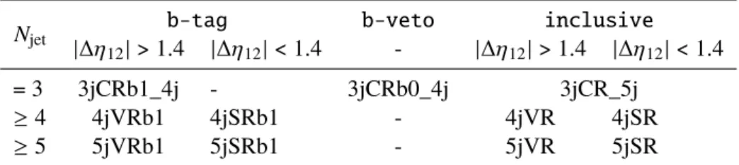
The selected events are divided into control, validation and signal regions, as summarized in Table1.
Control regions are defined with events that have three large-R jets with pT > 200 GeV. Additional requirements on the number of large-R jet with 100 GeV < pT < 200 GeV (soft large-Rjets) are used to separate control regions for events with different large-R jet multiplicities. For events with four or more large-Rjets (4j events), two control regions with a common requirement of at least one soft large-R jet being present are formed: one (3jCRb1_4j) consists ofb-tagevents and requires |∆η12| > 1.4, the other (3jCRb0_4j) consists ofb-vetoevents without requirement on|∆η12|. For events with five or more large-Rjets (5j events), one single control region (3jCR_5j) is defined by requiring the presence of at least two soft large-Rjets. Because of limited statistics of such events, this control region is not further divided based on number ofb-jets. For each control region, a variable binning in jetpTandηis chosen to ensure that every jet mass template has a sufficiently large number of jets.
Four overlapping signal regions (SRs) are considered in this analysis. All signal regions are required to have|∆η12|< 1.4. The first set of signal regions does not require the presence of ab-jet and is used to test more generic BSM signals of pair-produced heavy particles cascade decaying to many quarks or gluons.
Njet b-tag b-veto inclusive
|∆η12|> 1.4 |∆η12|< 1.4 - |∆η12|> 1.4 |∆η12|< 1.4
= 3 3jCRb1_4j - 3jCRb0_4j 3jCR_5j
≥4 4jVRb1 4jSRb1 - 4jVR 4jSR
≥5 5jVRb1 5jSRb1 - 5jVR 5jSR
Table 1: Control (CR), validation (VR), and signal (SR) regions used for the analysis.
Two selections on the large-R jet multiplicity are used, Njet≥ 4 (4jSR) and Njet≥ 5 (5jSR). To further improve the sensitivity to the benchmark signal models of RPV UDD scenario, subsets of events in the 4jSR and 5jSR are selected by requiring the presence of at least oneb-tagged small-Rjet. For each signal region, by reversing the|∆η12| requirement, a validation region is defined, which is used to cross check the background estimation, thus validating the background prediction in the signal region.
The background estimation performance is first examined in the validation region, before the signal region is unblinded.
Three main systematic uncertainties associated with the jet mass template method are considered. First, the jet mass template is created from a statistically limited jet sample and therefore the jet mass template is subject to statistical fluctuation. In addition, the jet mass randomization is statistical. The following procedure is used to propagate these statistical uncertainties to the predicted background yield for a given MΣ
J region. For each jet mass template, 1000 randomized templates are created by introducing bin-by-bin Poisson fluctuations to the template. These randomized templates are applied to the kinematic sample, generating 1000 randomized MΣ
J distributions. The central value of the predicted MΣ
J distribution is derived from the median prediction of these 1000 randomizedMΣ
J distributions, and the root-mean-square of the 1000 predictions is considered as the uncertainty due to the statistical fluctuation of jet mass templates and the jet mass randomization.
Second, thepTbin width used to create jet mass templates is finite, and the jet mass template has a residual pT-dependence in the samepTbin. The corresponding residualpT-dependence uncertainty is estimated by creating predictedMΣ
J distribution with intentionally mismatched jet kinematics and jet mass templates.
For example, for a jet withpT= 300 GeV, the jet mass template from 293 GeV < pT< 329 Ge should be used. Instead, the jet mass template from 329 GeV <pT < 364 GeV (or 270 GeV < pT < 293 GeV) is applied. The resultingMΣ
J distribution demonstrates the maximum effect of the residual pT-dependence uncertainty.
Third, the background estimation method is exercised in multi-jet Monte Carlo samples, and the difference between predicted and truth background yields is considered as a non-closure uncertainty for the jet mass template method. This non-closure uncertainty covers various other potential systematic uncertainties.
The differences found in the Pythia and Sherpa samples are consistent within statistical error, and the uncertainty derived from the Pythia sample is used due to the larger number of simulated events. The non-closure uncertainty derived from events with four or more large-Rjets is also applied to events with five or more large-Rjets, where the the Monte Carlo statistics is limited.
The potential bias on the background prediction due to signal contamination is studied with a Monte Carlo- based signal injection test. When the level of signal contamination is comparable to that predicted by signals of gluino direct or cascade decay models not yet excluded by Run-1, the predictedMΣ
J distribution
is insensitive to the contamination and shows good agreement with the background-onlyMΣ
J distribution.
If the level of signal contamination is significantly larger than that predicted by the benchmark signal models, an overestimation of background may appear. However, the predictedMΣ
J distribution is still well below theMΣ
J distribution of injected signal plus background, indicating that an excess of large signal will not be hidden by the overestimation.
Possible effects induced in the background estimation by the presence of massive objects from top pair production are not explicitly addressed by the background estimation strategy. However, a study similar to the one just described is performed to understand the potential effect of underestimating the contribution fromtt¯background, and the background prediction is found to be insensitive tot¯tcontamination as large as 3 times its theoretical prediction.
]-1Events / Bin width [TeV
10 102
103
104
105 ATLAS Preliminary Data Prediction
= 1600 GeV
g~
m = 650 GeV
0 χ∼1
m
= 1200 GeV
g~
m data 14.8 fb-1
≥ 4
largeR jet
N
| > 1.4 η
∆
| inclusive
[TeV]
Σ
MJ
0 0.2 0.4 0.6 0.8 1 1.2 1.4 1.6 1.8 2
Data/Pred
0 0.5 1 1.5 2
(a) ≥4 jets,inclusiveevents (4jVR)
]-1Events / Bin width [TeV
1 10 102
103
104
ATLAS Preliminary Data Prediction
= 1600 GeV
g~
m = 650 GeV
0 χ∼1
m
= 1200 GeV
g~
m data 14.8 fb-1
≥ 4
largeR jet
N
| > 1.4 η
∆
| b-tag
[TeV]
Σ
MJ
0 0.2 0.4 0.6 0.8 1 1.2 1.4 1.6 1.8 2
Data/Pred
0 0.5 1 1.5 2
(b) ≥4 jets,b-tagevents (4jVRb1)
]-1Events / Bin width [TeV
1 10 102
103
104
ATLAS Preliminary Data Prediction
= 1600 GeV
g~
m = 650 GeV
0 χ∼1
m
= 1200 GeV
g~
m data 14.8 fb-1
≥ 5
largeR jet
N
| > 1.4 η
∆
| inclusive
[TeV]
Σ
MJ
0 0.2 0.4 0.6 0.8 1 1.2 1.4 1.6 1.8 2
Data/Pred
0 0.5 1 1.5 2
(c) ≥5 jets,inclusiveevents (5jVR)
]-1Events / Bin width [TeV
1 10 102
103
ATLAS Preliminary Data Prediction
= 1600 GeV
g~
m = 650 GeV
0 χ∼1
m
= 1200 GeV
g~
m data 14.8 fb-1
≥ 5
largeR jet
N
| > 1.4 η
∆
| b-tag
[TeV]
Σ
MJ
0 0.2 0.4 0.6 0.8 1 1.2 1.4 1.6 1.8 2
Data/Pred
0 0.5 1 1.5 2
(d) ≥5 jets,b-tagevents (5jVRb1)
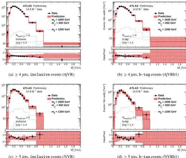
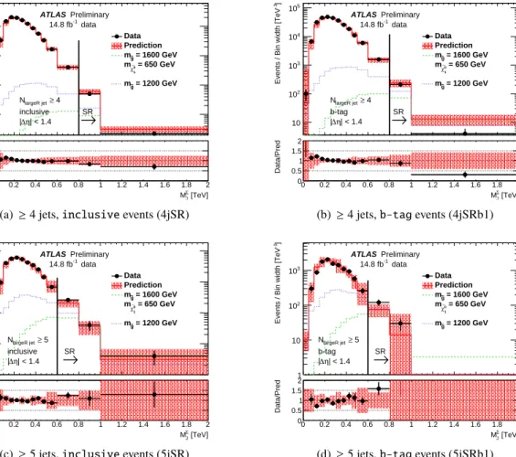
Figure 3: Predicted (solid line) and observed (dots)MΣ
J distributions for validation regions 4jVR(a), 4jVRb1(b), 5jVR(c), and 5jVRb1(d). The shaded area surrounding the predictedMΣ
J distribution represents the systematic uncertainty of the background estimation. The predicted MΣ
J distribution is normalized to data in 0.2 TeV <MΣ
J
< 0.6 TeV, where expected contamination from signals of gluino direct or cascade decay models not excluded by the Run-1 analysis [20] is negligible compared to the background statistical uncertainty. The expected contribution from two RPV signal samples are also shown.
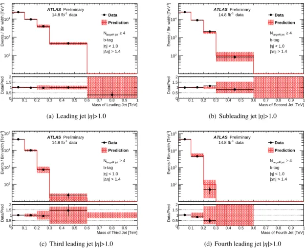
The jet mass template method is applied to data. The background estimation performance is first examined in the validation regions. Figure3shows the predicted and observed MΣ
J distributions in the validation regions, where in general a good agreement between the prediction and observation is seen. The modeling
of individual jet mass distribution is also checked for leading, subleading, third leading and fourth leading jets, separately for central jets (|η| < 1.0) and forward jets (|η| > 1.0), using events in the 4-jet validation regions (4jVR and 4jVRb1). No sign of mismodeling is found. Figure4shows the predicted and observed MΣ
J distributions in signal regions.
]-1Events / Bin width [TeV
102
103
104
105
ATLAS Preliminary Data Prediction
= 1600 GeV
g~
m = 650 GeV
0 χ∼1
m
= 1200 GeV
g~
m data 14.8 fb-1
≥ 4
largeR jet
N
| < 1.4 η
∆
|
inclusive SR
→
[TeV]
Σ
MJ
0 0.2 0.4 0.6 0.8 1 1.2 1.4 1.6 1.8 2
Data/Pred
0 0.5 1 1.5 2
(a) ≥4 jets,inclusiveevents (4jSR)
]-1Events / Bin width [TeV
10 102
103
104
105
ATLAS Preliminary Data Prediction
= 1600 GeV
g~
m = 650 GeV
0 χ∼1
m
= 1200 GeV
g~
m data 14.8 fb-1
≥ 4
largeR jet
N
| < 1.4 η
∆
|
b-tag SR
→
[TeV]
Σ
MJ
0 0.2 0.4 0.6 0.8 1 1.2 1.4 1.6 1.8 2
Data/Pred
0 0.5 1 1.5 2
(b)≥4 jets,b-tagevents (4jSRb1)
]-1Events / Bin width [TeV
1 10 102
103
104 ATLAS Preliminary Data Prediction
= 1600 GeV
g~
m = 650 GeV
0 χ∼1
m
= 1200 GeV
g~
m data 14.8 fb-1
≥ 5
largeR jet
N
| < 1.4 η
∆
|
inclusive SR
→
[TeV]
Σ
MJ
0 0.2 0.4 0.6 0.8 1 1.2 1.4 1.6 1.8 2
Data/Pred
0 0.5 1 1.5 2
(c) ≥5 jets,inclusiveevents (5jSR)
]-1Events / Bin width [TeV
1 10 102
103
ATLAS Preliminary Data Prediction
= 1600 GeV
g~
m = 650 GeV
0 χ∼1
m
= 1200 GeV
g~
m data 14.8 fb-1
≥ 5
largeR jet
N
| < 1.4 η
∆
|
b-tag SR
→
[TeV]
Σ
MJ
0 0.2 0.4 0.6 0.8 1 1.2 1.4 1.6 1.8 2
Data/Pred
0 0.5 1 1.5 2
(d)≥5 jets,b-tagevents (5jSRb1)
Figure 4: Predicted (solid line) and observed (dots) MΣ
J distributions for signal regions 4jSR (a), 4jSRb1 (b), 5jSR(c), and 5jSRb1(d). The shaded area surrounding the predictedMΣ
J distribution represents the systematic uncertainty of background estimation. The predictedMΣ
J distribution is normalized to data in 0.2 TeV <MΣ
J < 0.6 TeV, where expected contamination from signals of gluino direct or cascade decay models not excluded by the Run-1 analysis [20] is negligible compared to the background statistical uncertainty. The expected contribution from two RPV signal samples are also shown.
Many tests are performed using the control regions as well as validation regions in order to determine the robustness of the method. These tests include creating separate jet mass templates for different types of jets (leading, subleading, etc.), applying jet mass templates created from control regions without additional soft large-R jet requirement to validation regions with different jet multiplicities, creating separate jet mass templates for large-Rjets that can be matched to ab-jet and large-Rjets that cannot be matched to a b-jet, varying thepTandηbinning of the control samples, and varying the binning of jet mass templates.
The predictedMΣ
J distribution is compared to the observed one in both signal and control regions in these tests. It is found that the variation in the predicted yield is within the estimated uncertainties.
The statistical interpretation is based on the event yield in a signal region beyond an MΣ
J threshold. For
5jSR and 5jSRb1, the threshold used onMΣ
J is 0.6 TeV, while it is 0.8 TeV for 4jSR and 4jSRb1. These thresholds were found to give the maximum sensitivity to both gluino direct and cascade decay models.
The model-dependent interpretation uses data in the 5jSRb1 with MΣ
J > 0.6 TeV, which has the best sensitivity among four signal regions.
6 Signal systematic uncertainties
The main systematic uncertainties for the predicted signal yield include the large-R jet mass scale and resolution uncertainties,b-tagging uncertainty, Monte Carlo statistical uncertainty, and luminosity uncer- tainty. The large-Rjet mass scale and resolution uncertainty is as large as 24% for signal models with mg˜ = 1000 GeV, and drops to≈ 8% for signal models withmg˜ =1800 GeV. The Monte Carlo samples reproduce the b-tagging efficiency measured in data with limited accuracy. Dedicated correction factors, derived from a comparison between data and MC int¯t events, are applied to the signal samples. The uncertainty of the correction factors is propagated to a systematic uncertainty on the yields in the signal region. This uncertainty is at around 3% level for all signal models considered in this analysis. Due to low acceptance, the statistical uncertainty of the signal yield predicted by the Monte Carlo samples can be as large as 8% for signal models withmg˜ ≤1000 GeV. The Monte Carlo statistical uncertainty for signal models with largemg˜ is negligible.
Uncertainties on the signal acceptance due to the choices of PDF, QCD scales and the modeling of initial state radiation (ISR) are studied. The uncertainty of PDF and QCD scales is found to be up to 20%
for mg˜ ≈ 1000 GeV, and a few percent for mg˜ ≈ 1600 GeV. Since the signal samples are generated at the leading order, the ISR modeling uncertainty is evaluated by varying αs used in the Pythia parton showering up and down by 10 %. This uncertainty is found to be up to 10 % at aroundmg˜ = 1000 GeV, and a few percent at aroundmg˜ = 1600 GeV and beyond.
7 Results
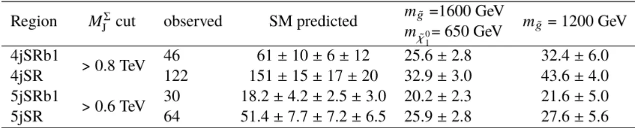
Table2summarizes the predicted and observed event yields in signal regions with differentMΣ
J cuts. No excess is seen in the≥4 jets signal regions (4jSR and 4jSRb1), and small excesses are seen in ≥ 5 jets signal regions (5jSR and 5jSRb1).
The predicted and observed event yields shown in Table2are used to construct a likelihood function, where signal and background systematic uncertainties are incorporated as nuisance parameters. A likelihood function is constructed with the observed and predicted yields shown in Table2, with signal and background systematic uncertainties incorporated as nuisance parameters. A frequentist procedure based on the profile likelihood ratio [61] is used to evaluate thep0-values of these excesses, and the results are shown in Table3.
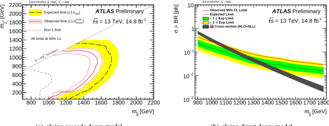
Since no significant excess is seen in any of the signal regions, a model-independent limit onσvis, defined as the cross section times acceptance times efficiency of a generic BSM model, is calculated using the modified frequentistC Ls method [62]. The observed and expected limits are also shown in Table3.
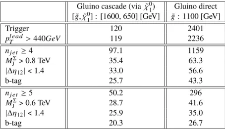
Limits are also set on the production of RPV signals in the context of gluino direct and cascade decay models and are shown in Figure5. Typically, for RPV signals from the gluino cascade decay model with mg˜ ≥ 1000 GeV, the ratio of the detector level acceptance over truth level acceptance is between 0.95 and 1.10, for 4jSR withMΣ
J > 0.8 TeV and 5jSR with MΣ
J > 0.6 TeV. For signal regions withb-tagging