Jet energy scale and its systematic uncertainty in proton-proton collisions at √

ATLAS-CONF-2013-004 29/01/2014

ATLAS NOTE

ATLAS-CONF-2013-004

January 26, 2013

Minor revision: January 27, 2014

Jet energy scale and its systematic uncertainty in proton-proton collisions at √

s = 7 TeV with ATLAS 2011 data

The ATLAS Collaboration

Abstract

The jet energy scale (JES) and its systematic uncertainty are determined for jets mea- sured with the ATLAS detector using proton-proton collision data with a centre-of-mass energy of

√

s =

7 TeV corresponding to an integrated luminosity of 4.7 fb

⁻¹

. Jets are re- constructed from topological clusters of calorimeter cells using the anti-k

t

algorithm with distance parameters

R=

0.4 or

R=

0.6, and are calibrated using Monte Carlo simulation. A residual JES correction is applied to account for di

ff

erences between data and Monte Carlo.

This correction and its systematic uncertainty are evaluated in bins of jet pseudorapidity and transverse momentum, for jets with calibrated transverse momenta

p^jet_T >

20 GeV and pseudorapidities

|η| <

4.5. They are estimated using a combination of

in situ

techniques exploiting the transverse momentum balance between a jet and a reference object such as a photon or a

Z

boson for 20

≤ p^jet_T <

1000 GeV. The effect of multiple proton-proton interac- tions is corrected for and an uncertainty is evaluated using

in situ

techniques. The smallest JES uncertainty of less than 1% is found in the central calorimeter region (

|η| <

1.2) for jets with 55

≤ p^jet_T <

500 GeV. For central jets at lower

p_T

the uncertainty is about 3%. A consistent JES estimate is found using

in situ

single hadron response measurements and test beam results, which provide the estimate for

p^jet_T >

1 TeV. The calibration of forward jets (|η|

>

1.2) is derived from dijet

p_T

balance measurements. The resulting uncertainty reaches its largest value of 6% for low-p

_T

jets at

|η| =

4.5. Additional JES uncertainties due to specific event topologies, such as close-by jets or from selections of event samples with different compositions of jets originating from light quarks versus those originating from gluons, are also discussed. The magnitude of these uncertainties depends on the event sample used in a given physics analysis, but typically amounts to 0.5-3%.

Revised labels of figure 7 with respect to the version of January 26, 2013 c

Copyright 2013 CERN for the benefit of the ATLAS Collaboration.

Reproduction of this article or parts of it is allowed as specified in the CC-BY-3.0 license.

1 Introduction

Jets are the dominant feature of high energy, hard proton-proton interactions at the Large Hadron Col- lider (LHC) at CERN. They are key ingredients for many physics measurements and for searches for new phenomena. Jets are observed as groups of topologically-related energy deposits in the ATLAS calorimeters associated with tracks of charged particles as measured in the inner detector. They are typ- ically reconstructed with the anti-k

t

jet algorithm [1] and are calibrated using Monte Carlo simulation (MC). Only jets reconstructed with this algorithm and with distance parameters of R

=

0.4 and R

=

0.6 will be covered in this note. Reference [2] describes the calibration and performance of non-standard jets that have been constructed using di

ff

erent clustering algorithms and distance parameters.

A first estimate of the jet energy scale (JES) uncertainty, described in Ref. [3], was based on infor- mation available before the first LHC collisions and exploited in addition transverse momentum balance in events with only two jets at high transverse momenta (p

_T

) produced in situ. A reduced uncertainty of about 2.5% in the central calorimeter region over a wide momentum range of 60

.

p

_T <

800 GeV was achieved based on the increased knowledge of the detector performance obtained during the analysis of the first year of data taken with the ATLAS detector [4]. This estimation used single hadron calorimeter response measurements [5], systematic Monte Carlo simulation variations, and in situ techniques, where the jet transverse momentum is compared to the p

_T

of a reference object. These measurements were done using the 2010 dataset consisting of 7 TeV pp collisions, corresponding to an integrated luminosity of 38 pb

⁻¹

.

During 2011, the ATLAS detector collected proton-proton collision data at a centre-of-mass energy of

√

s

=

7 TeV with a corresponding integrated luminosity of about 4.7 fb

⁻¹

. This much larger dataset makes it possible to further improve the precision of the jet energy measurement and also to apply cor- rections derived from detailed comparisons of data and Monte Carlo simulation using in situ techniques.

This document presents the results of the calibration of the jet energy measurement and the determination of the uncertainties.

The outline of the note is as follows: Sections 2-4 describe the ATLAS detector, the dataset, and the Monte Carlo (MC) simulation framework. Section 5 briefly summarises the jet reconstruction and calibration strategy and Section 6 explains the strategy used for obtaining and applying the in situ cali- bration techniques. These techniques are outlined in Section 7 and are described in detail elsewhere in Refs. [6–9]. The associated uncertainties for each in situ method are also presented. Section 8 presents the final jet energy calibration and its uncertainty from the combination of the in situ techniques. Sec- tion 9 compares the JES uncertainty as derived from the single hadron calorimeter response measure- ments to the one from the in situ method based on p

_T

-balance.

Jet energy scale uncertainties considered in addition to the baseline JES as derived from the in situ techniques are discussed in Section 10. These include uncertainties due to jet fragmentation, specific to jets initiated by light quarks or gluons (see Section 10.1), or due to special event topologies as in the case of close-by jets (see Section 10.3). The effect of extra energy due to multiple proton-proton interactions (pile-up) is discussed in Section 10.4. A summary of the total jet energy scale uncertainty is given in Section 11.

2 The ATLAS detector

The ATLAS detector consists of a tracking system (Inner Detector, or ID in the following) in a 2 T solenoidal magnetic field up to a pseudorapidity

¹ |η| <

2.5, sampling electromagnetic and hadronic

1The ATLAS Coordinate System is a right-handed system with thex-axis pointing to the centre of the LHC ring, thez-axis following the beam direction and they-axis pointing upwards. The pseudorapidityηis an approximation for rapidityyin the high energy limit, and it is related to the polar angleθasη=−ln tan^θ₂.

calorimeters up to

|η|<

4.9, and muon chambers in a toroidal magnetic field, covering a pseudorapidity range

|η| <

2.5. A detailed description of the ATLAS experiment can be found elsewhere [10].

Tracks of charged particles are reconstructed using information from the layers of silicon pixel detec- tors, silicon microstrip detectors, and transition radiation tracking detectors, all of which are immersed in the 2 T magnetic field from the solenoid.

Jets are reconstructed using the ATLAS calorimeter detectors, whose granularity and material varies as a function of

η. The electromagnetic calorimetry is provided by high granularity liquid argon (LAr)

sampling calorimeters using lead as an absorber that are split into barrel (|η|

<

1.475) and end-cap (1.375

< |η| <

3.2) regions. The hadronic calorimeter is divided into three distinct regions: the barrel region (|η|

<

0.8) and the extended barrel region (0.8

<|η|<

1.7) instrumented with a tile scintillator/steel calorimeter; the Hadronic End-Cap region (HEC; 1.5

<|η|<

3.2) using LAr

/

copper calorimeter modules, and finally the Forward Calorimeter region (FCal; 3.1

< |η| <

4.9) instrumented with LAr/copper and LAr/tungsten modules to provide electromagnetic and hadronic energy measurements, respectively.

3 Dataset

The dataset considered was collected with all ATLAS subdetectors operational. It corresponds to a total integrated luminosity of about 4.7 fb

⁻¹

of proton-proton collisions at a centre-of-mass energy of

√

s

=

7 TeV, collected between April and October of 2011.

The LHC was operated with a bunch crossing-interval (bunch spacing) of 50 ns, and bunches were organised in bunch trains. The average number of interactions per bunch crossing (µ) was 3

≤ µ ≤

8 until summer 2011, with an average for this period of

µ ≈

6. Starting in August 2011 and up until the end of the proton run, the

µ

range increased to about 5

≤µ≤

17, with an average

µ≈

12 [11].

4 Monte Carlo simulation of jets in the ATLAS detector

The nominal simulation samples are produced with the event generator P

ythia

[12], which simulates proton-proton collisions using a set of 2

→

2 matrix elements at leading order in the strong coupling to model the hard subprocess, and uses p

_T

-ordered parton showers to model additional radiation in the leading-logarithm approximation [13]. Multiple parton interactions [14], as well as fragmentation and hadronisation based on the Lund string model [15], are also simulated. The parton shower and multiple parton interactions in the underlying event are generated using the Pythia AUET2B tune to first 2011 data [16] and the MRST LO** parton density function (PDF) has been used [17].

Samples to evaluate systematic uncertainties are based on the H

erwig++

[18] event generator that also uses a set of leading-order 2

→

2 matrix elements with angular-ordered parton showers in the leading-logarithm approximation [19–21], together with the cluster model for hadronisation [22]. A mixture of soft and hard multiple partonic interactions [23] is used to model the underlying event and soft inclusive interactions. The ATLAS MC11 AUET2 tune [16] with the MRST LO** PDF set [17] is used.

The nominal samples for t¯ t events were produced using the MC@NLO v4.01 [24] generator with the CT10 PDF set [25]. The parton shower and the underlying event were added using the HERWIG v6.520 [26] and JIMMY 4.31 [27] generators, together with the ATLAS AUET2 LO** tune [16]. Other t¯ t samples used for the calculation of systematic uncertainties have been simulated using POWHEG [28]

interfaced to either Pythia or to HERWIG and JIMMY, and with the AcerMC generator [29] interfaced to P

ythia

.

The Monte Carlo samples are all produced including additional minimum bias interactions, using

Pythia with the ATLAS MC11 AUET2B CTEQ6L1 tune [30] and CTEQ6L PDF set [31]. These min-

imum bias events are used to form pile-up events, which are overlaid onto the hard scattering events

following a Poisson distribution around the average number of additional proton-proton collisions per bunch crossing measured in the experiment. The LHC bunch train structure is also modeled in that the simulated collisions are organised in four trains with 50 ns spacing between the bunches. Additional proton-proton collisions from nearby bunch crossings within trains of consecutive bunches (out-of-time pile-up) are simulated. Monte Carlo simulation samples are then weighted such that the distribution of the average number of interactions per bunch crossing matches the data distribution.

The G

eant

4 software toolkit [32] within the ATLAS simulation framework [33] propagates the gen- erated particles through the ATLAS detector and simulates their interactions with the detector material.

Hadronic showers are simulated with the QGSP BERT model [34–42]. Compared to the simulation used for the 2010 data analysis, a newer version of G

eant

4 (version 9.4) is used and a more detailed description of the geometry of the LAr calorimeter is introduced.

Dag Gillberg, Carleton Jet calibration schemes 2012-09-05 6

Calorimeter jets

(EM or LCW scale) Pile-up offset

correction Origin correction Energy & ! calibration

Residual in situ calibration

Calorimeter jets (EM+JES or LCW+JES scale)

Jet calibration

Changes the jet direction to point to the primary vertex.

Does not affect the energy.

Calibrates the jet energy and pseudorapidity to the particle jet scale.

Derived from MC.

Residual calibration derived using in situ measurements.

Derived in data and MC.

Applied only to data.

Corrects for the energy offset introduced by pile-up.

Depends on µ and NPV. Derived from MC.

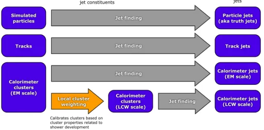
Jet reconstruction

jet constituents jets

Local cluster weighting

Calorimeter clusters (LCW scale) Calorimeter

clusters (EM scale)

Jet finding Calorimeter jets (LCW scale)

Jet finding Calorimeter jets

(EM scale)

Tracks Track jets

Simulated particles

Particle jets (aka truth jets)

Calibrates clusters based on cluster properties related to shower development

Jet finding Jet finding

Figure 1: Overview of the ATLAS jet reconstruction. After the jet finding, the jet four momentum is defined as the four momentum sum of its constituents.

Dag Gillberg, Carleton Jet calibration schemes 2012-09-05 6

Calorimeter jets (EM or LCW scale)

Pile-up offset

correction Origin correction Energy & ! calibration

Residual in situ calibration

Calorimeter jets (EM+JES or LCW+JES scale)

Jet calibration

Changes the jet direction to point to the primary vertex.

Does not affect the energy.

Calibrates the jet energy and pseudorapidity to the particle jet scale.

Derived from MC.

Residual calibration derived using in situ measurements.

Derived in data and MC.

Applied only to data.

Corrects for the energy offset introduced by pile-up.

Depends on µ and NPV. Derived from MC.

Jet reconstruction

jet constituents jets

Local cluster weighting

Calorimeter clusters (LCW scale) Calorimeter

clusters (EM scale)

Jet finding Calorimeter jets (LCW scale)

Jet finding Calorimeter jets

(EM scale)

Tracks Track jets

Simulated particles

Particle jets (aka truth jets)

Calibrates clusters based on cluster properties related to shower development

Jet finding Jet finding

Figure 2: Overview of the ATLAS jet calibration scheme used for the 2011 dataset. The pile-up, absolute JES and the residual in situ corrections calibrate the scale of the jet, while the origin and the

η

corrections affect the direction of the jet.

5 Jet reconstruction and calibration in the ATLAS detector

Jets are reconstructed using the anti-k

t

algorithm [1] with distance parameters R

=

0.4 or R

=

0.6 using the F

ast

J

et

software [43, 44]. The four-momentum recombination scheme is used. The input to the jet algorithm are stable simulated particles

²

(truth jets), reconstructed tracks in the inner detector (track

2A particle is defined as stable if its lifetime is longer than 10 ps. Muons and neutrinos are not included as input to truth jets as they interact weakly with the detector.

det| η Jet |

0 0.5 1 1.5 2 2.5 3 3.5 4 4.5

Jet response at EM scale

0.3 0.4 0.5 0.6 0.7 0.8 0.9 1

E = 30 GeV E = 60 GeV E = 110 GeV

E = 400 GeV E = 2000 GeV HEC-FCal FCal

Transition Barrel-Endcap HEC

Transition Barrel

= 0.4, EM+JES

tR : Anti-k 2011 JES

Preliminary ATLAS

Simulation

(a) EM-scale

det| η Jet |

0 0.5 1 1.5 2 2.5 3 3.5 4 4.5

Jet response at LCW scale

0.5 0.6 0.7 0.8 0.9 1 1.1 1.2

E = 30 GeV E = 60 GeV E = 110 GeV

E = 400 GeV E = 2000 GeV HEC-FCal FCal

Transition Barrel-Endcap HEC

Transition Barrel

= 0.4, LCW+JES

tR : Anti-k 2011 JES

Preliminary ATLAS

Simulation

(b) LCW-scale

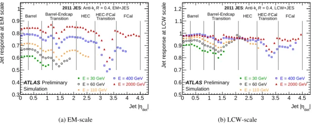
Figure 3: Average energy of jets formed from topo-clusters calibrated at EM (a) or LCW scale (b) with respect to the truth jet energy (E

_jet^EM/LCW/E_jet^truth

) as a function of the jet pseudorapidity before applying the correction for the event vertex shown separately for various jet energies. Also indicated are the different calorimeter regions. The inverse of the response shown in each bin is equal to the average jet energy scale correction. This result is based on Pythia inclusive jet samples.

jets) or energy deposits in the calorimeter (calorimeter jets). A schematic overview of the ATLAS jet reconstruction is presented in Figure 1.

The calorimeter jets used in this note are reconstructed from topological calorimeter clusters (topo- clusters) [4, 45, 46] with a positive energy. The topo-clusters are built from topologically connected calorimeter cells that contain a significant signal above noise. To account for the increased contribu- tion from overlaid minimum bias events (pile-up) fluctuations, the cell noise thresholds have been in- creased [47]. The contribution from electronic noise is added in quadrature with the contribution from pile-up fluctuations corresponding to an average of eight additional proton-proton interactions per bunch crossing (µ

=

8).

The topo-clusters are reconstructed at the EM scale [45, 48–55], which correctly measures the en- ergy deposited by particles produced in electromagnetic showers in the calorimeter. The clusters can thereafter be calibrated using the local cluster weighting (LCW) method that aims at an improved resolu- tion compared to the EM scale, reducing fluctuations due to the non-compensating nature of the ATLAS calorimeter. LCW first classifies topo-clusters as either electromagnetic or hadronic, primarily based on the measured energy density and the longitudinal shower depth. Energy corrections are derived according to this classification from single charged and neutral pion Monte Carlo simulations. Dedicated correc- tions are derived for the e

ff

ects of calorimeter non-compensation, signal losses due to noise threshold effects, and energy lost in non-instrumented regions [4].

Figure 2 presents an overview of the ATLAS calorimeter jet calibration scheme used for the 2011 dataset, which restores the jet energy scale to that of jets reconstructed from stable simulated particles (truth particle level). This procedure consist of four steps as described below.

1. Jets formed from topo-clusters at the EM or LCW scale are first calibrated by applying a correction

to account for the energy offset caused by pile-up interactions. The effects of pile-up on the jet

energy scale are caused by both additional proton collisions in a recorded event (in-time pile-up)

and by past and future collisions influencing the energy deposited in the current bunch-crossing

(out-of-time pile-up), and are outlined in Section 10.4. This correction [47] is derived from Monte

Carlo simulations as a function of the number of reconstructed primary vertices (N

PV

, measuring

the actual collisions in a given event) and the expected average number of interactions (µ, sensitive to out-of-time pile-up) in bins of jet pseudorapidity and transverse momentum.

2. A correction to the calorimeter jet direction is applied that makes the jet point back to the primary event vertex instead of the centre of the ATLAS detector.

3. The jet energy calibration is derived as a simple correction relating the reconstructed jet energy to the truth jet energy [4]. It can be applied to jets formed from topo-clusters at EM-scale or at LCW-scale with the resulting jets being referred to as calibrated with the EM+JES or with the LCW

+

JES scheme. This first JES correction is derived for isolated jets from a inclusive jet Monte Carlo sample including pile-up events (the baseline sample described in Section 4). Figure 3 shows the average energy response

R=

E

^EM/LCW_jet /E_jet^truth

, which is equal to the inverse of the jet calibration, for various jet energies as a function of the jet pseudorapidity.

³

4. A residual in situ derived correction is applied as a last step to jets reconstructed in data. The derivation of this correction is described in the following sections.

6 Strategy to derive the in situ jet energy calibration and uncertainty

After the first JES calibration step described in point 3 of Section 5, the jet p

_T

( p

^jet_T

) in data is compared to the one in Monte Carlo simulation using in situ techniques that exploit the p

_T

balance

⁴

between the jet p

_T

and the p

_T

of a reference object (p

^ref_T

):

D

p

^jet_T /p^ref_T E

data/D

p

^jet_T/

p

^ref_T E

MC

(1)

This quantity is the residual in situ JES correction for jets measured in data. It is derived as follows:

•

Firstly, the average p

_T

for jets within 0.8

≤ |η|<

4.5 is equalised to the p

_T

of jets within

|η| <

0.8 exploiting the p

_T

balance between a central and a forward jet in events with only two jets at high p

_T

(dijet

η-intercalibration, see Section

7.1).

•

After the pseudorapidity dependence of the jet response is removed by the dijet

η-intercalibration,

the in situ JES correction for jets within

|η| <

1.2

⁵

is derived using the p

_T

of a photon or a Z boson (decaying to e

⁺

e

⁻

or

µ⁺µ⁻

) as reference (see Section 7.2). The JES correction is obtained from a combination of both methods (γ

+jet and

Z

+jet) and the corresponding JES uncertainty is

determined from the uncertainties of each in situ technique (see Section 7.3). This correction and relative uncertainties are applied also to jets in the endcap and forward region, evaluated for

η ≥

1.2 and

η≤

-1.2.

•

Finally, events where a system of low-p

T

jets recoils against a high- p

_T

jet are used to calibrate jets in the TeV regime. The low-p

T

jets are within

|η| <

2.8 while the leading jet is required to be within

|η| <

1.2. The uncertainties from the low-p

_T

jets derived from

γ+

jet, Z

+

jet and dijet p

_T

balance (see Section 7.3) are propagated to high p

_T

jets.

3The quantityηdetdenotes the jet pseudorapidity before applying a correction for the event vertex, i.e. the jet direction is measured with respect to the centre of the detector.

4It should be noted that the two objects are not expected to exactly balance due to e.g. intial-state radation and out-of-cone energy. These effects are simulated in the Monte Carlo. This is further discussed in Section7.3.

5Thein situmethods focusing on the central region are not limited to using the reference region|η| <0.8 used by the dijet η-intercalibration. The slightly larger interval|η| <1.2 provides more statistics while still keeping systematic uncertainties small.

The in situ JES corrections and the corresponding JES uncertainty for jets within

|η| <

1.2 are hence derived from a combination of the

γ+

jet, Z

+

jet and multijet techniques. The derivation of this correction is explained in Section 8. The JES uncertainties for forward jets 1.2

≤ |η|<

4.5 are derived from those for central jets

|η| <

1.2 using the dijet

η-intercalibration technique.

7 Jet energy calibration and uncertainty from in situ transverse momen- tum balance techniques

7.1 Relative in situ calibration between the central and forward rapidity regions

The transverse momentum balance in dijet events is exploited to study the pseudorapidity dependence of the jet response. A relative

η-intercalibration is derived using the so-called

matrix method [6] to correct the jets in data for residual e

ff

ects not captured by the initial Monte Carlo simulation derived calibration.

This analysis covers jets with 20

≤

p

^jet_T <

1500 GeV and

|η|

up to 4.5. Jets up to

|η|=

2.8 are calibrated using

|η| <

0.8 as a reference region. For jets with

η >

2.8 (η <

−2.8), for which the uncertainty on the

derived calibration becomes large, the calibration measured at

η=

2.8 (η

= −2.8) is used⁶

. Jets that fall in the reference region receive on average no additional correction. The

η-intercalibration is applied to

all jets prior to deriving the absolute in situ calibration described in the subsequent sections.

The largest uncertainty of the dijet balance technique is due to the modelling of the additional parton radiation altering the dijet balance. This uncertainty is estimated using the Pythia and Herwig++ Monte Carlo simulations.

7.2 In situ calibration methods for the central rapidity region

The energy scale of jets is tested in situ using a well-calibrated object as reference. The following techniques are used for the central rapidity region

|η| <

1.2:

1.

Direct p_Tbalance between a photon or aZboson and a jet

Events with a photon or a Z boson and a recoiling jet are used to compare the transverse momen- tum of the jet to that of the photon or the Z boson [7, 8]. This method is called direct balance (DB).

The data is compared to the Monte Carlo simulation in the jet

η

range

|η| <

1.2. The

γ+

jet analy- sis covers a range in photon transverse momentum from 25 to 800 GeV, while the Z

+jet analysis

covers a range in Z boson transverse momentum from 15 to 200 GeV. However, only the results involving a Z boson are used in the derivation of the residual JES correction, as the method em- ploying p

_T

balance between a photon and the hadronic recoil (see next item) is used in place of the

γ+

jet DB as explained in Section 8.2.

2.

pTbalance between a photon and the hadronic recoil

The photon transverse momentum is balanced against the full hadronic recoil using the projection of the missing transverse momentum onto the photon direction. This method, called missing transverse momentum projection fraction (MPF) technique [8], measures the calorimeter response for the hadronic recoil, which is independent of the jet algorithm. The comparison is done in the same kinematic region as the direct photon balance method.

3.

Balance between a system of low-pTjets and a high-pTjet

Jets at high p

_T

can be balanced against a recoil system of low p

_T

jets within

|η| <

2.8, if the low-p

T

jets are well calibrated using

γ+jet or

Z

+jet

in situ techniques. The multijet balance can be iterated several times to increase the subleading jet p

_T

range beyond the values covered by

γ+

jet or

6The relative jet response is measured independently for each side of the detector.

Z

+jet balance and reaching higher

p

_T

of the leading jet, until the low number of events precludes a precise measurement. This method can probe the jet energy scale up to the TeV-regime [9].

The numbers of events available in the full dataset after all selection cuts for each in situ technique are summarized in Table 1.

The mean transverse momentum sum of tracks within a cone around the jet direction provides an independent test of the calorimeter energy scale over the entire measured p

^jet_T

range within the tracking acceptance. This method described in Ref. [4] used for the 2010 dataset was also studied for the inclu- sive jet data sample in 2011 [56]. However, because of the relatively large systematic uncertainty, it is presently not included in the JES combination.

Table 1: Summary of the number of events available for various in situ techniques after all selection cuts.

The numbers are given for illustration in specific p

^jet_T

ranges for anti-k

t

jets with R

=

0.4 reconstructed with the EM+JES scheme. The

γ+jet results are based on the MPF method.

Z

+

jet method

p

^jet_T

20

−

25 GeV 35

−

45 GeV 210

−

260 GeV

Number of events 8530 8640 309

γ+

jet method

p

^jet_T

25

−

45 GeV 45

−

65 GeV 210

−

260 GeV 600

−

800 GeV

Number of events 20480 61220 10210 100

multijet method

p

^jet_T

0.21

−

0.26 TeV 0.75

−

0.95 TeV 1.45

−

1.8 TeV

Number of events 2638 3965 48

7.3 Uncertainty sources of the in situ calibration techniques

The in situ techniques usually rely on assumptions that are only approximately fulfilled: an example is the assumption that the calibrated jet and the reference object are balanced in transverse momentum, while this balance can be altered by the presence of additional high-p

_T

particles. In order to determine the JES uncertainties, the modelling of physics effects has to be disentangled from detector effects. These effects can be studied by systematically varying the event selection criteria. The ability of the Monte Carlo simulation to describe large variations of the selection criteria determines the systematic uncertainty in the in situ methods, since physics e

ff

ects can be suppressed or amplified by these variations. In addition, systematic uncertainties related to the selection, calibration and modelling of the reference object need to be considered.

When performing the variations of the selection criteria, only statistically significant variations of the response ratios are propagated to the systematic uncertainties. This is achieved by evaluating the systematic uncertainties in intervals which can be larger than the bins used for the measurement of the response ratios (several bins are iteratively combined until the observed deviations are significant). By doing so, one avoids multiple counting of the statistical uncertainties in the systematics that are evaluated.

Using this procedure, the radiation suppression uncertainty for the

∆φγ,jet

cut on the MPF method [8] has been dropped

⁷

.

7This uncertainty is very small, and the corresponding variations are not significant, even when the evaluation is performed on the fullpTrange.

For the relative

η-intercalibration (see Sec.

7.1), the dominant uncertainty source is due to MC mod- elling of jets at forward rapidities, where properties di

ff

er for the generators considered (P

ythia

and Herwig). Other systematic uncertainty sources arise due to the modelling of the jet resolution, the trig- ger, and dijet topology selection. However, these components are negligible when compared to the MC modelling uncertainty.

The data-to-MC response ratio (as defined in Eq. 1) for the direct balance in Z

+jet events, the MPF

technique in

γ+jet events, and the multijet balance method are combined (see Sec.

8). In this combina- tion, the ability of the Monte Carlo simulation to describe the data, the individual uncertainties of the in situ techniques and their compatibility are considered. The uncertainties of the three central in situ methods combined here are described by a set of 54 systematic uncertainty sources listed in Table 2. The photon and electron energy scale uncertainties are treated as being fully correlated at this level. Com- ponents directly related to the dijet balance technique are

η-dependent quantities, and are thus treated

differently. Such parameters are not included in the list of 54 components, although uncertainties related to their propagation through other methods are included.

In Table 2, each uncertainty component has been assigned to one of four categories, based on its source and correlations:

•

Detector description (labelled det.)

•

Physics modelling (model)

•

Statistics and method (stat.

/

meth.)

•

Mixed detector and modelling (mixed).

For the combination of measurements from two different experiments, it is suggested to consider the uncertainty components in the detector and statistics and method cathegory as uncorrelated, while the uncertainties in the modelling cathegory are likely to contain components that are correlated between the two experiments. For the mixed detector and modelling categories the correlations between experiments need more studies to be determined in a quantitative way. In the absence of further studies the correlations between experiments should be treated in a conservative way, by testing several possible hypothesis for the correlations, and choosing the one which produces the largest uncertainty on the final distribution.

8 Jet energy calibration and uncertainty combination

8.1 Combination technique

The data to Monte Carlo simulation response ratios (see Eq. 1) of the various in situ methods are com- bined using the procedure described in Sec. 10.5 of Ref. [4]. The in situ jet response measurements are made in bins of p

^ref_T

and are evaluated at the barycentre

hp^ref_T i

of each bin.

⁸

First, a common, fine p

_T

binning (to be used for the combination result) is defined. In each p

_T

-bin, and for each in situ method that contributes to that bin, the data-to-MC response ratio is determined using interpolating splines based on second order polynomials. The combined data-to-MC ratio in each bin is determined by a weighted average of the interpolated contributions from the various in situ methods.

The weights are obtained by a

χ²

minimisation of the response ratios in each p

_T

bin, and are therefore proportional to the inverse of the square of the uncertainties of the input measurements. The local

χ²

is also used to test the level of agreement between the in situ methods.

8SinceD p^jet_T/p^ref_T E

is close to unity for all p^ref_T -bins, the bin barycentreD p^ref_T E

is a good approximation ofD p^jet_TE

. In the followingp^jet_T is used.

Name Description Category Common sources

Electron/photon E scale electron or photon energy scale det.

Z

+jet

p

_T

balance (DB)

MC generator MC generator di

ff

erence between A

lpgen/

H

erwig

and P

ythia

model Radiation suppression radiation suppression due to second jet cut model Extrapolation extrapolation in

∆φ_jet

-

^Z

between jet and Z boson model Pile-up jet rejection jet selection using jet vertex fraction mixed

Out-of-cone contribution of particles outside the jet cone model

Width width variation in Poisson fits to determine jet response stat./meth.

Statistical components statistical uncertainty for each of the 11 bins stat.

/

meth.

γ+

jet p

_T

balance (MPF)

MC Generator MC generator di

ff

erence H

erwig

and P

ythia

model

Radiation suppression sensitivity to radiation suppression due to second jet cut model Jet resolution variation of jet resolution within uncertainty det.

Photon Purity background response uncertainty and photon purity estimation det.

Pile-up sensitivity to pile-up interactions mixed

Out-of-cone contribution of particles outside the jet cone model

Statistical components statistical uncertainty for each of the 12 bins stat.

/

meth.

Multijet p

_T

balance

α

selection angle between leading jet and recoil system model

β

selection angle between leading jet and closest sub-leading jet model Dijet balance dijet balance correction applied for

|η| <

2.8 mixed Close-by, recoil JES uncertainty due to close-by jets in the recoil system mixed

Fragmentation jet fragmentation modelling uncertainty mixed

Jet p

_T

threshold jet p

_T

threshold mixed

p

_T

asymmetry selection p

_T

asymmetry selection between leading jet and sub-leading jet model UE,ISR/FSR soft physics effects modelling: underlying event and soft radiation mixed Statistical components statistical uncertainty for each of the 10 bins stat.

/

meth.

Table 2: Summary table of the uncertainty components for each in situ technique (Z

+

jet [7],

γ+

jet [8]

and multijet p

_T

balance [9]) used to derive the jet energy scale uncertainty. Each uncertainty component

is also categorized depending on its source as either: detector (labelled det.), physics modelling (labelled

model), mixed detector and modelling (labelled mixed), or as statistics and method (labelled stat.

/

meth.).

Each uncertainty source of the in situ methods is treated as fully correlated across p

_T

and

η. The

uncertainty sources are assumed to be independent of each other. The full set of uncertainties are propa- gated from the in situ methods to the combined result in each p

_T

bin using pseudo-experiments [4]. For some applications (combination/comparison of several experimental measurements etc.) it is necessary to understand the contribution of each uncertainty component to the final total uncertainty. For this pur- pose, each uncertainty component is propagated separately from each in situ method to the combined result. This is achieved by coherently shifting all the correction factors obtained by the in situ meth- ods by one standard deviation of a given uncertainty component, and redoing the combination using the same set of averaging weights as in the nominal combination. The comparison of the shifted average correction factors with the nominal ones provides the propagated systematic uncertainty.

To account for potential disagreement between in situ measurements constraining the same term (referred to as measurements which are ’in tension’), each uncertainty source is rescaled by the factor

pχ²/dof, if this factor is larger than 1. This is conservative, as values of p

χ²/dof larger than 1 can also

be reached due to statistical fluctuations.

The combined data-to-MC response ratio is used as the in situ correction calibration factor and is applied to data. The correction factor still contains part of the statistical fluctuations of the in situ mea- surements. The influence of the statistical fluctuations is reduced by applying a minimal amount of smoothing using a sliding Gaussian kernel to the combined correction factors [4].

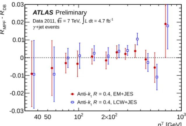
8.2 Comparison of the in situ γ + jet calibration methods

Two different in situ techniques exploiting the transverse momentum balance in

γ+jet events are used

to probe the jet response: the direct balance (DB) and the Missing Momentum fraction (MPF) method (see Section 7.2). These methods have di

ff

erent sensitivity to parton radiation, pile-up interactions and photon background contamination, and hence different systematic uncertainties [8].

Since the MPF method uses the full hadronic recoil and not only the jet, a systematic uncertainty due to the possible di

ff

erence in data and Monte Carlo simulation of the calorimeter response to particles inside and outside of the jet needs to be taken into account. This systematic uncertainty contribution is estimated to be small compared to other considered uncertainties. However, in the absence of a more quantitative estimation, the full energy of all particles produced outside of the jet as estimated in the DB technique is taken as the systematic uncertainty. A comparison between the two results is shown in Figure 4. The results are compatible within their uncorrelated uncertainties.

As the methods use similar datasets, the measurements are highly correlated and cannot easily be included together in the combination of the in situ techniques. In order to judge which method results in the most precise calibration, the in situ combination described in Section 8.1 was performed twice, both for Z

+

jet,

γ+

jet DB and multijet balance, and separately for Z

+

jet,

γ+

jet MPF and multijet balance. The resulting combined calibration that includes the MPF method has slightly smaller uncertainties (by up to about one per mill), and is therefore used as the main result.

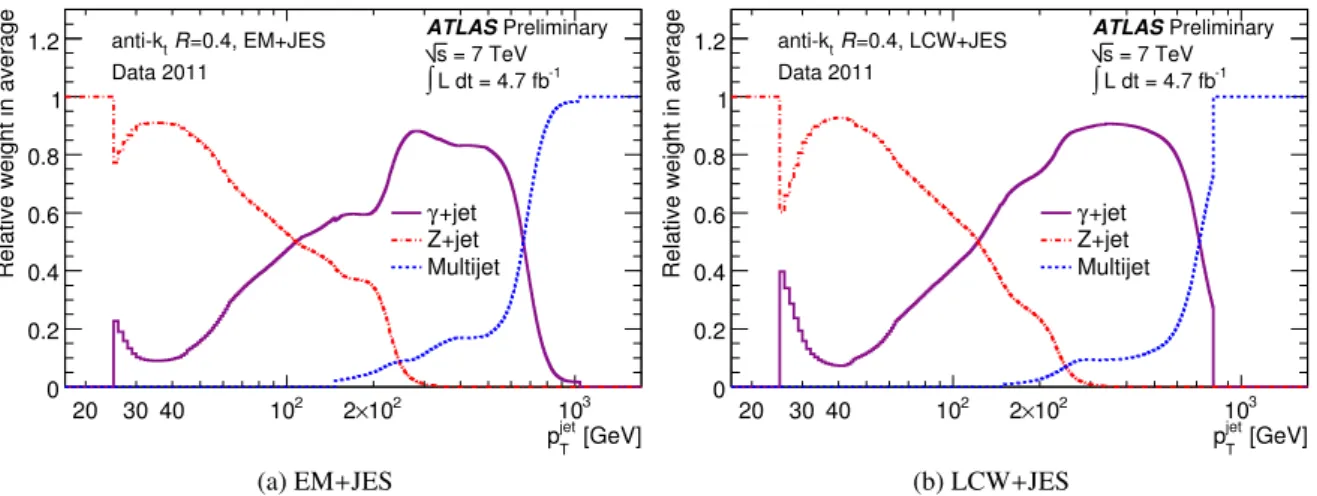
8.3 Combination results

Figure 5 shows the contribution of each in situ technique to the JES residual calibration defined to be the fractional weight carried in the combination. In the region p

^jet_T .

100 GeV, the Z

+

jet method has the highest contribution to the overall JES average. The contribution is 100% for p

^jet_T

below 25 GeV (in the region covered only by Z

+

jet), about 90% at p

^jet_T =

40 GeV and decreases to about 50% at p

^jet_T =

100 GeV.

In order to prevent the uncertainties specific to the low p

^jet_T

region from propagating to higher p

^jet_T

in the

combination, the Z

+

jet measurements below and above p

^jet_T =

25 GeV are treated separately (i.e. no

interpolation is performed across p

^jet_T =

25 GeV, although the magnitude of the original systematic un-

[GeV]

γ

pT

40 50 10² 2×10² 10³

DBR - MPFR

-0.03 -0.02 -0.01 0 0.01 0.02 0.03

ATLAS Preliminary dt = 4.7 fb-1

L = 7 TeV, s

Data 2011, ∫

+jet events γ

= 0.4, EM+JES

tR k Anti-

= 0.4, LCW+JES

tR k Anti-

Figure 4: Di

ff

erence between the data

/

MC response ratio R measured using the direct balance (DB) and the missing momentum fraction (MPF) methods for jets reconstructed with the anti-k

t

algorithm with R

=

0.4 calibrated with the EM+JES and LCW+JES schemes. The error bars shown only contain the uncorrelated uncertainties.

certainty sources is used, separately, in both regions). The weaker correlations between the uncertainties of the Z

+jet measurements, compared to ones from γ+jet, lead to a faster increase of the extrapolated

uncertainties, hence to the reduction of the Z

+

jet weight in the region between 25 and 40 GeV. In the region 100

.

p

^jet_T .

600 GeV the

γ+

jet method dominates with a weight increasing from 50% at p

^jet_T =

100 GeV to about 80% at p

^jet_T =

500 GeV. For p

^jet_T &

600 GeV the measurement based on multijet balance becomes increasingly important and for p

^jet_T &

800 GeV it is the only method contributing to the JES residual calibration. The combination results and the relative uncertainties are considered in the p

_T

range 17.5 GeV - 1 TeV, where sufficient statistics is available.

The individual uncertainty components for the final combination results

⁹

, are shown in Fig. 6 for anti-k

t

jets with R

=

0.4 for the EM

+

JES and the LCW

+

JES calibration scheme and for each in situ technique.

The agreement between the in situ methods is good, with

χ²/dof values below 1 for most

p

_T

bins and values up to

χ²/dof=

1.5 in a few bins. The largest

χ²/dof =

2 is found for anti-k

t

jets with R

=

0.6 calibrated with the LCW+JES scheme for p

^jet_T =

25 GeV.

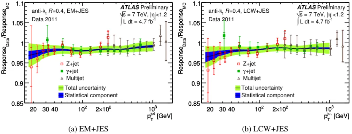
The final JES residual calibration obtained from the combination of the in situ techniques is shown in Figure 7 together with statistical and systematic uncertainties. A general o

ff

set of about

−2% is

observed between the data and MC response ratios for jet transverse momenta below 100 GeV. The offset decreases to about

−1% at higher

p

_T

(p

^jet_T &

200). The JES uncertainty from the combination of the in situ techniques is about 2.5% at p

^jet_T =

25 GeV, and decreases to below 1% for 55

≤

p

^jet_T <

500 GeV. The multijet balance method is used up to 1 TeV, as at higher p

_T

values it has large statistical uncertainties.

At 1 TeV the total uncertainty is about 1.5%.

The results for the EM+JES and the LCW+JES calibration schemes for jets with R

=

0.6 are similar to those for R

=

0.4.

9The uncertainties apply to the overall result of the combination of thein situtechniques and differ from the original uncertainties of the in-situ methods as they have been convoluted with the corresponding weights.

[GeV]

jet

pT

20 30 40 10² 2×10² 10³

Relative weight in average

0 0.2 0.4 0.6 0.8 1 1.2

γ+jet Z+jet Multijet

=0.4, EM+JES

tR anti-k Data 2011

ATLASPreliminary = 7 TeV s

∫ ^-1

L dt = 4.7 fb

(a) EM+JES

[GeV]

jet

pT

20 30 40 10² 2×10² 10³

Relative weight in average

0 0.2 0.4 0.6 0.8 1 1.2

γ+jet Z+jet Multijet

=0.4, LCW+JES

tR anti-k Data 2011

ATLASPreliminary = 7 TeV s

∫ ^-1

L dt = 4.7 fb

(b) LCW+JES

Figure 5: Weight carried by each in situ technique in the combination to derive the residual jet energy scale calibration as a function of the jet transverse momentum p

^jet_T

for anti-k

t

jets with R

=

0.4 calibrated with the EM

+

JES (a) and the LCW

+

JES (b) scheme. The p

^jet_T

dependence of the weights is discussed in Section 8.3.

8.4 Simplified description of the correlations

For some applications (e.g. parametrised likelihood fits) it is preferable to have the JES uncertainties and correlations described by a reduced set of uncertainty components. In this section we describe a method to reduce the number of uncertainty components while maintaining a sufficient accuracy for the JES uncertainty correlations.

The total covariance matrix C

^tot

of the JES correction factors can be derived from the individual components of the statistical and systematic uncertainties:

C

^tot=

Nsources

X

k=1

C

^k,

(2)

where the sum goes over the covariance matrices of the individual uncertainty components C

^k

. Each uncertainty component s

^k

is treated as fully correlated in p

_T

and the covariance of the p

_T

-bins i and j is given by C

^k_{i j} =

s

^k_i

s

^k_j

. All the uncertainty components are treated as independent between each other, except for the photon and electron energy scales which are treated as correlated

¹⁰

.

A reduction of the number of nuisance parameters while retaining the information on the correlations can be achieved by deriving the total covariance matrix (see Eq. 2) and diagonalizing it:

C

^tot=

S

^T

D S. (3)

Here D is a (positive definite) diagonal matrix, containing the eigenvalues (σ

²_k

) of the total covariance ma- trix, while the S matrix contains on its columns the corresponding (orthogonal) unitary eigenvectors (V

^k

).

A new set of independent uncertainty sources can then be obtained by multiplying each eigenvector by the corresponding eigenvalue. The covariance matrix can be rederived from these uncertainty sources

10The photon and electron energy scales are first added linearly, the corresponding fully correlated covariance matrix is derived and added linearly to the covariance matrix of the other uncertainty components. In other words, a single systematic uncertainty source is assigned to account for both the photon and electron energy scales.

[GeV]

jet

pT

20 30 40 10² 2×10² 10³

Relative uncertainties

0 0.005 0.01 0.015 0.02 0.025 0.03

=0.4, EM+JES

tR anti-k Data 2011

ATLASPreliminary

|<1.2 η = 7 TeV, | s

∫ ^-1

L dt = 4.7 fb -scale

Electron E Extrapolation Pile-up jet rejection Out-of-cone MC generator Radiation suppression Width

Statistical components Z+jet

(a) EM+JESZ+jet DB

[GeV]

jet

pT

20 30 40 10² 2×10² 10³

Relative uncertainties

0 0.005 0.01 0.015 0.02 0.025 0.03

=0.4, LCW+JES

tR anti-k Data 2011

ATLASPreliminary

|<1.2 η = 7 TeV, | s

∫ ^-1

L dt = 4.7 fb -scale

Electron E Extrapolation Pile-up jet rejection Out-of-cone MC generator Radiation suppression Width

Statistical components Z+jet

(b) LCW+JESZ+jet DB

[GeV]

jet

pT

20 30 40 10² 2×10² 10³

Relative uncertainties

0 0.005 0.01 0.015 0.02 0.025 0.03

=0.4, EM+JES

tR anti-k Data 2011

ATLASPreliminary

|<1.2 η = 7 TeV, | s

∫ ^-1

L dt = 4.7 fb -scale

Photon E Photon purity Pile-up MC generator Jet resolution Out-of-cone Radiation suppression Statistical components γ+jet

(c) EM+JESγ+jet MPF

[GeV]

jet

pT

20 30 40 10² 2×10² 10³

Relative uncertainties

0 0.005 0.01 0.015 0.02 0.025 0.03

=0.4, LCW+JES

tR anti-k Data 2011

ATLASPreliminary

|<1.2 η = 7 TeV, | s

∫ ^-1

L dt = 4.7 fb -scale

Photon E Photon purity Pile-up MC generator Jet resolution Out-of-cone Radiation suppression Statistical components γ+jet

(d) LCW+JESγ+jet MPF

[GeV]

jet

pT

20 30 40 10² 2×10² 10³

Relative uncertainties

0 0.005 0.01 0.015 0.02 0.025 0.03

=0.4, EM+JES

tR anti-k Data 2011

ATLASPreliminary

|<1.2 η = 7 TeV, | s

∫ ^-1

L dt = 4.7 fb selection

α selection β

Dijet balance Close-by, recoil Fragmentation

threshold Jet pT

asymmetry selection pT

UE, ISR/FSR Statistical components Multijet

(e) EM+JES Multijet

[GeV]

jet

pT

20 30 40 10² 2×10² 10³

Relative uncertainties

0 0.005 0.01 0.015 0.02 0.025 0.03

=0.4, LCW+JES

tR anti-k Data 2011

ATLASPreliminary

|<1.2 η = 7 TeV, | s

∫ ^-1

L dt = 4.7 fb selection

α selection β

Dijet balance Close-by, recoil Fragmentation

threshold Jet pT

asymmetry selection pT

UE, ISR/FSR Statistical components Multijet

(f) LCW+JES Multijet

Figure 6: Individual uncertainty sources applicable to the combined response ratio as a function of the jet p

_T

for the three in situ techniques: Z

+

jet direct balance (a,b),

γ+

jet MPF (c,d) and multijet balance (e,f) for anti-k

t

jets with R

=

0.4 calibrated with the EM+JES (a,c,e) and the LCW+JES (b,d,f) scheme.

The systematic uncertainties displayed here correspond to the components listed in Table 2.

[GeV]

jet

pT

20 30 40 10² 2×10² 10³

MC/ResponseDataResponse

0.85 0.9 0.95 1 1.05 1.1

=0.4, EM+JES

tR anti-k Data 2011

ATLASPreliminary

|<1.2 η = 7 TeV, | s

∫ ^-1

L dt = 4.7 fb

Z+jet γ+jet Multijet Total uncertainty Statistical component

[GeV]

jet

pT

20 30 40 10² 2×10² 10³

MC/ResponseDataResponse

0.85 0.9 0.95 1 1.05 1.1

(a) EM+JES

[GeV]

jet

pT

20 30 40 10² 2×10² 10³

MC/Response DataResponse

0.85 0.9 0.95 1 1.05 1.1

=0.4, LCW+JES

tR anti-k Data 2011

ATLASPreliminary

|<1.2 η = 7 TeV, | s

∫ ^-1

L dt = 4.7 fb

Z+jet γ+jet Multijet Total uncertainty Statistical component

[GeV]

jet

pT

20 30 40 10² 2×10² 10³

MC/Response DataResponse

0.85 0.9 0.95 1 1.05 1.1

(b) LCW+JES

Figure 7: Ratio of the average jet response

hp^jet_T /p^ref_T i

measured in data to that measured in MC for jets within

|η| <

1.2 as a function of the transverse jet momentum p

^jet_T

. The data-MC jet response ratios are shown separately for the three in situ techniques used in the combined calibration: direct balance in Z

+jet events, MPF inγ+jet events, and multijet

p

_T

balance in inclusive jet events. The error bars indicate the statistical and the total uncertainties (adding in quadrature statistical and systematic uncertainties).

Results are shown for anti-k

t

jets with R

=

0.4 calibrated with the EM

+

JES (a) and the LCW

+

JES (b) scheme. The light band indicates the total uncertainty from the combination of the in situ techniques.

The inner dark band indicates the statistical component only.

using:

C

_{i j}^tot=

Nbins

X

k=1

σ²_k

V

_i^k

V

^k_j,

(4)

where N

_bins

is the number of bins used in the combination.

A good approximation of the covariance matrix can be obtained by separating out only a small subset of N

_eff

eigenvectors that have the largest corresponding eigenvalues. From the remaining N

_bins−

N

_eff

components, a residual, left-over uncertainty source is determined, with an associated covariance matrix C

⁰

. The initial covariance matrix can now be approximated as:

C

^tot_{i j} ≈

Neff

X

k=1

σ²_k

V

_i^k

V

^k_j +

C

⁰.

(5)

This approximation conserves the total uncertainty, while the precision on the description of the correla- tions can be directly determined by comparing the original full correlation matrix and the approximate one. The last residual uncertainty could in principle be treated either as correlated or as uncorrelated between the p

_T

-bins. It is observed that treating this uncertainty source as uncorrelated in p

_T

provides a better approximation of the correlation matrix. This is expected, as this residual uncertainty source includes many (small amplitude) orthogonal eigenvectors with many oscillations (hence the small corre- lations). In other words, the original exact covariance matrix can be decomposed into a part with strong correlations and another one with much smaller correlations. It is this residual uncertainty source that incorporates the part with small correlations.

Fig. 8 shows the obtained five eigenvectors

σ_k

V

^k

and the residual sixth component, as a function of

the jet p

_T

, that are enough to describe the correlation matrix with su

ffi

cient (percent level) precision. As

explained above, the quadratic sum of these six components is identical to the quadratic sum of the orig-

inal uncertainties in Fig. 6. In the high p

_T

region (above 300 GeV), one eigenvector has a significantly