Monte Carlo Calibration and Combination of In-situ Measurements of Jet Energy Scale, Jet Energy Resolution and Jet Mass in ATLAS

A TLAS-CONF-2015-037 17 August 2015

ATLAS NOTE

ATLAS-CONF-2015-037

17th August 2015

Monte Carlo Calibration and Combination of In-situ Measurements of Jet Energy Scale, Jet Energy Resolution and Jet Mass in ATLAS

The ATLAS Collaboration

Abstract

The various stages in the final Run-1 jet energy scale calibration in the ATLAS detector at the Large Hadron Collider are described. The Monte Carlo based calibration is discussed for both small (R = 0.4 or 0.6) and large (R ≥ 1.0) radius jets and the final combination of various in-situ measurements and the resultant jet energy scale uncertainty is presented. An uncertainty on the jet energy calibration of less than 1% is acheived for small-radius jets with

|η| < 0.8 and 150 < p _T < 1500 GeV. The mass scale calibration of large radius jets is also discussed with its associated uncertainties which are around 4% in the central region for jets with 200 < p _T < 2000 GeV. Next, two novel methods to measure the noise component of the jet energy resolution in small radius jets are discussed, which have a measurement precision of 20%. Finally, the combination of in-situ measurements of the jet energy resolution for small jets and the associated uncertainties are presented with a total jet energy resolution uncertainty of 1% above 100 GeV and less than 3% at 20 GeV. The joint effect of the jet energy resolution combination and direct noise measurements allows a first extraction of distinct noise, stochastic and constant resolution terms.

c

2015 CERN for the benefit of the ATLAS Collaboration.

Reproduction of this article or parts of it is allowed as specified in the CC-BY-3.0 license.

1 Introduction

Collimated sprays of energetic hadrons, known as jets, are the dominant final state objects of high-energy proton-proton (pp) interactions at the Large Hadron Collider (LHC) at CERN. They are key ingredients for many physics measurements and for searches for new phenomena. Jets are observed as groups of topologically-related energy deposits in the ATLAS [1] calorimeters. Jets are reconstructed by first clustering energy deposits into “topological clusters” and then clustering these using either the anti-k t [2], k t or the Cambridge/Aachen (C/A) [3, 4] jet algorithms. The same algorithms can also be used to create jets from other inputs, such as inner detector tracks associated with charged particles.

Jets are calibrated to the energy scale of truth jets created using the same clustering algorithm from stable interacting particles in Monte Carlo ¹ . The calibration has to account for several different effects;

1. Calorimeter non-compensation: correction for the different scales of the energy measured from hadronic and electromagnetic showers.

2. Dead material: energy lost in inactive areas of the detector.

3. Leakage: showers reaching the outer edge of the calorimeters.

4. Out of calorimeter jet: energy of particles which are included in the truth jet but which are not included in the reconstructed jet.

5. Energy deposits below noise thresholds: clusters are only formed by energy deposits which are well above the background noise. Therefore the correction is required to correct for particles that do not form clusters. Additionally some part of a shower may fall outside of the topological clusters such that this also needs to be corrected for.

6. Pile-up: energy deposition in jets is a ff ected by the presence of multiple pp collisions in the same bunch crossing as well as residual signals from other bunch crossings.

This calibration scales the jets to the truth jet energy scale and the uncertainty on this scaling in the data forms one of the major systematics in many ATLAS analyses [5, 6]. The calibration is derived using a combination of methods based on Monte Carlo (MC) simulation and data-driven techniques. The data are used through data-driven methods to derive a small residual calibration correction and constrain the uncertainty in the calibration.

In 2012, ATLAS collected events from pp collisions at a centre-of-mass energy of √

s = 8 TeV, with a total dataset corresponding to approximately 20 fb ⁻¹ of integrated luminosity. Such a large data set is essential for analyses searching for evidence of new phenomena, as well as for precision measurements of the Standard Model. However, with increased luminosity the beam conditions in 2012 were more challenging than those delivered in 2011. The ability to mitigate the e ff ects of additional interactions was key to the good performance of the detector in 2012.

This note details the Monte Carlo based calibration of jets and the combination of various in-situ studies of the jet energy scale and resolution. Following a brief description of the detector in Section 2 and the Monte Carlo simulation samples in Section 3, in Section 4 the reconstruction algorithms for jets used in 2012 are described. The calibration of these jets is then described in Section 5. Section 6 details the determination and combination of in-situ studies of the jet calibration using dijet and Z/γ + jet events. Section 7 summarises the uncertainty on the jet calibration. Section 8 presents studies of the jet energy resolution (JER) following the calibration schemes discussed. Finally, Section 9 presents the

1 Truth particles are particles in Monte Carlo which are considered stable if they have a lifetime greater than 30 ps. A truth

particle is considered to be interacting if it is expected to deposit most of its energy in the ATLAS calorimeters; truth muons

and neutrinos are considered to be non-interacting.

combination of in-situ studies of JER and details the resulting uncertainties on the resolution of jets in ATLAS.

2 The ATLAS detector

The ATLAS detector consists of an inner tracking detector, sampling electromagnetic and hadronic calorimeters, and muon chambers in a toroidal magnetic field. A detailed description of the ATLAS experiment can be found elsewhere [1].

The inner detector (ID) has complete azimuthal coverage and spans the region |η| < 2.5. ² It consists of layers of high-granularity silicon pixel detectors, silicon microstrip detectors and transition radiation tracking detectors. These detectors are immersed in a solenoid magnet that provides a uniform magnetic field of 2 T. The ID is used to reconstruct tracks from charged particles and determine their transverse momenta from the curvature of the tracks.

Jets are reconstructed from energy deposited in the ATLAS calorimeter system. Electromagnetic calorimetry is provided by high granularity liquid argon (LAr) sampling calorimeters, using lead as an absorber, which are split into barrel (|η| < 1.475) and endcap (1.375 < |η| < 3.2) regions. In addition, inside this layer of calorimeters, a LAr based presampler layer is included which allows corrections for energy loss due to showers initiated by material before the calorimeters. The hadronic calorimeter is di- vided into the barrel (|η| < 0.8) and two extended barrel (0.8 < |η| < 1.7) regions, which are instrumented with scintillator tile/steel calorimeters and the hadronic endcap region (1.5 < |η| < 3.2), which uses LAr/copper calorimeter modules. The forward calorimeter region (3.1 < |η| < 4.9) is instrumented with LAr / copper and LAr / tungsten modules to provide electromagnetic and hadronic energy measurements, respectively. The electromagnetic and hadronic calorimeters are segmented in layers, allowing a deter- mination of the longitudinal profiles of showers. The electromagnetic barrel, the electromagnetic endcap first wheel and Tile calorimeters consist of three layers. The electromagnetic endcap second wheel con- sists of two layers. The hadronic endcap calorimeters consists of four layers. The forward calorimeters have one electromagnetic and two hadronic layers.

The muon spectrometer surrounds the ATLAS calorimeter. A system of three large air-core toroids (each with 8 coils), a barrel and two endcaps, generates a magnetic field in the pseudorapidity range of

|η| < 2.7. The muon spectrometer measures muon tracks with three layers of precision tracking chambers and is instrumented with separate trigger chambers.

Events are retained for analysis using the ATLAS trigger system that consists of a hardware-based

“level 1 trigger” (L1) followed by a software-based “higher level trigger” (HLT) [7]. Jets are first iden- tified at L1 using a sliding window algorithm that takes coarse granularity calorimeter towers as input.

This is refined using jets reconstructed from calorimeter cells in the HLT.

3 MC Simulation

Monte Carlo event generators are used to simulate the energy and direction of particles produced in pp collisions. An overview of the MC event generators used in ATLAS can be found in Ref. [8].

The dijet simulation samples used to derive the JES calibration, the Global Sequential (GS) correc- tion [9], and the in-situ calibrations are produced with the P ythia 8 [10] event generator. The simulation uses a 2 → 2 matrix element interfaced with the CT10 [11] parton density function (PDF) to model the hard subprocess, and p _T -ordered parton showers to model additional radiation in the leading-logarithmic

2 The ATLAS coordinate system is right-handed, with the x-axis pointing to the centre of the LHC ring, the z-axis following

the beam direction and the y-axis pointing upwards. The azimuthal angle φ = 0 corresponds to the positive x-axis and φ

increases clockwise looking into the positive z direction. The pseudorapidity η is an approximation for rapidity, y, in the high

energy limit, and it is related to the polar angle θ as η = − ln tan ^θ ₂ .

approximation. The AU2 tune [12] is used to model the underlying event (UE). Multiple parton inter- actions (MPI) as well as fragmentation and hadronisation based on the Lund string model [13] are also simulated.

Samples used to evaluate the flavour response and in-situ systematic uncertainties are based on the Herwig ++ MC event generator [14, 15]. Herwig ++ uses a 2 → 2 matrix element and angular-ordered parton showers in the leading-logarithm approximation and the cluster model for the hadronisation [8].

The underlying event (UE) and soft inclusive interactions are described using a hard and soft MPI model [16].

Further samples are used in the in-situ methods used to study jets using the balance against a reference object. Details of these samples are given in Refs. [17, 18] and so, are not repeated here.

Pile-up e ff ects in all samples are modeled using simulated minimum bias events generated using Pythia8. These events are overlaid onto the hard scattering events following a Poisson distribution around the average number of additional pp collisions per bunch crossing, µ. The effects from pile-up events occurring in nearby bunch crossings (out-of-time pile-up) are also modeled by overlaying the hard scattering event with simulated detector signals from P ythia 8 minimum bias events. These overlaid events are sampled from out-of-time bunches according to a simulation of the LHC bunch train structure.

Generated events are propagated through a full simulation of the ATLAS detector [19] based on G eant 4 [20] that simulates the interactions of the particles produced by the event generators with the detector material. Hadronic showers are simulated with the QGSP BERT model [21].

Due to the large number of MC events required by many physics analyses, the Atlfast-II (AFII) fast simulation [22] is often used to produce MC samples. In this note, fast simulation versions of the samples discussed above are also used to investigate the differences in jets reconstructed in full and fast simulation. AFII uses a simplified modelling of the calorimeter simulation which allows a factor of ten more events to be produced for the same CPU time. The standard ATLAS reconstruction algorithms are used to reconstruct simulated events produced with fast simulation.

4 Jet Reconstruction

Jets are reconstructed using the anti-k t algorithm [2] with radius parameters R = 0.4, R = 0.6 or R = 1.0 or the Cambridge/Aachen (C/A) algorithm [3, 4] with radius parameter R = 1.2 using the F ast J et software [23, 24]. The inputs to the jet algorithm are either stable simulated “truth” particles, energy deposits in the calorimeter or tracks in the inner detector, and the resulting jets are referred to as truth jets, calorimeter jets or track jets, respectively.

Truth jets are reconstructed using the same algorithm as calorimeter jets, but using truth particles with a lifetime greater than 30 ps as input, excluding muons and neutrinos. Only calorimeter and truth jets with p ^jet _T > 7 GeV and |η| < 4.5 are used in the derivation of the calibration.

Track jets are built using inner detector tracks which are reconstructed within the full acceptance of the ID, |η| < 2.5. Track reconstruction begins from “hits”, namely charge deposits from charged particles in the ID sub-detectors. A sequence of algorithms is used to build tracks from individual hits [25]. The baseline algorithm uses 3-point seeds in the silicon detectors (Pixel and SCT) to form track candidates, which are then extrapolated to include TRT measurements. Tracks are required to have transverse mo- mentum of at least 400 MeV, in addition to further quality criteria relating to impact parameters and numbers of hits in the di ff erent ID sub-detectors.

The inputs to calorimeter jets are topological clusters of calorimeter cells [26–28] (topo-clusters)

constructed from adjacent calorimeter cells that contain a significant energy signal above noise. These are

treated as massless particles and are assumed to originate from the geometrical center of the detector. The

topo-clusters are initially reconstructed at the electromagnetic scale (EM-scale) [29–32], which correctly

measures the energy deposited in the calorimeter by particles produced in electromagnetic showers.

A second topo-cluster collection is built by taking the previous EM scale collection and calibrating the calorimeter cells in these clusters such that the response of the calorimeter to hadrons is correctly accounted for. This calibration uses the local cluster weighting (LCW) method that aims at an improved resolution compared to the EM scale by correcting for a variety of effects in the calorimeter; firstly clus- ters are classified as electromagnetic or hadronic such that the non-compensating nature of the ATLAS calorimeter can be accounted for, secondly the energy falling outside clustered cells is estimated from how isolated the cluster is, and finally the amount of energy falling in inactive areas of the detector is estimated from the position and energy deposited in each layer of the calorimeter [27]. LCW corrections are determined from Monte Carlo simulations of charged and neutral pions.

For flavour studies, the highest energy parton that points to the jet (i.e. with ³ ∆ R < 0.6 for jets with R = 0.6 and ∆ R < 0.4 for jets with R = 0.4) determines the flavour of the jet. Jets identified as originating from heavy (c and b) quarks (HQ-jets) are considered separately from jets originating from light quarks (LQ-jets) or gluons. This definition is sufficient to study the flavour dependence of the jet response. Any theoretical ambiguities of jet flavour assignment are not relevant in this context. Jets originating from the parton shower and thus not matched to any parton from the matrix element are not used for these studies [27].

4.1 Jet Selection

Calorimeter jets are required to satisfy the “looser” quality criteria discussed in detail in Ref. [33]. Any event containing a jet that fails the “looser” quality criteria is rejected.

A ∆ R matching method is used to compare reconstructed calorimeter jets to truth particle jets in sim- ulation. Calorimeter jets are required to geometrically match truth jets within a certain angular distance

∆ R of the calorimeter jet axis. Matching is performed in order of decreasing reconstructed jet p _T , dis- carding jets that have already been matched; ambiguities are resolved by choosing the truth jet with the highest p _T as the match. The matching radius used is ∆ R = 0.3. Jets are required to be isolated, i.e. there should be no other reconstructed jets with p _T > 7 GeV at the uncalibrated scale within a cone of ∆ R = 1.5 × R. Similarly, there should be no other truth jets with p ^truth _T > 7 GeV within a cone of ∆ R = 2.5 × R.

The jet response is defined using the associated particle jet kinematics and is defined as

R = hp ^jet _T /p ^truth _T i. (1)

Unless stated otherwise, in the rest of the note we refer to the mean and standard deviation of the Gaussian fit ⁴ to the response distribution as “jet response”, R, and “jet resolution”, σ R /R, respectively.

5 Jet Energy Calibration

The calibration procedure used in 2012 is based on an extension of the procedure detailed in Ref. [34] and is shown schematically in Figure 1. First a jet is corrected to point back to the correct vertex as detailed in Section 5.1. Next the effect of pile-up is removed using an area based subtraction process discussed in Section 5.2. The jet energy is then calibrated by applying the jet energy scale (JES) derived from MC and discussed in Section 5.3. In addition to these steps, further corrections are applied to the jets which reduce the difference in response between gluon and quark initated jets and also correct for jets which are not fully contained in the calorimeter. These additional corrections form the global sequential correction scheme (GSC) and are outlined in Section 5.4. Next, the di ff erence between the jet energy scale in full and fast simulation is discussed in Section 5.5. Finally, the calibration of large R = 1.0 jets is discussed

3 ∆R is the sum in quadrature of the difference in pseudorapidity, ∆η, and the difference in azimuth, ∆φ: ∆R = p ( ∆η) ² + ( ∆φ) ² .

4 performed over ±1.5σ down to a minimum E T > 8.5 GeV.

in Section 5.6. The final stage of the calibration, the residual in-situ calibration, will be discussed in Section 6.

Dag Gillberg, Carleton Jet calibration schemes 09/02/2015

Jet calibration scheme

1

Residual in-situ calibration EM or LCW

constituent scale jets Residual pile-up

correction

Absolute EtaJES

Origin Correction

Global sequential calibration

Jet area based pile- up correction

Function of µ and NPV
 applied to the jet at

constituent scale Function of event pile-up

energy density and jet area Jet finding applied to

topological clusters at EM or LCW scale

Changes the jet direction to point to the primary vertex. Does not affect E.

Corrects the jet 4-vector to the particle level scale.

Both the energy and direction are calibrated.

Based on tracking and muon activity behind jets.

Reduces flavour dependence and energy leakage effects.

A final residual calibration is derived using in-situ

measurements and is applied only to data

Figure 1: The stages used in the calibration of EM and LCW jets.

5.1 Origin Correction

The ATLAS calorimeters measure the energy of particles. Topo-clusters therefore require to be assigned a direction to complete their 4-vector. The default choice is to point them at the center of the detector, however, following reconstruction of the full event a better assumption is that they originated from the position of the “first primary vertex” ⁵ . The origin correction accounts for this di ff erence by finding the energy center of the jet and then modifying the jet 4-vector such that the energy is unchanged but the direction originates from the “first primary vertex”.

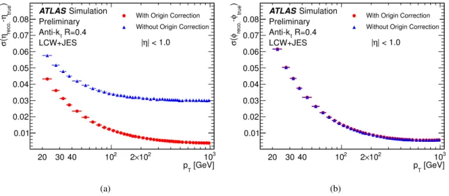
This procedure results in a dramatic improvement in the η resolution of jets due to the length of the beamspot along the beamline, which had a luminous size of between 40-55 mm in 2012. This improvement is shown in Figure 2. Also shown in Figure 2 is the resolution in φ for completeness.

There is little change in the resolution in φ before and after the origin correction due to the small spread of the beam-spot in x, y.

[GeV]

p

20 30 40 10

2 × 10

10

)

η -

η ( σ

0.01 0.02 0.03 0.04 0.05 0.06 0.07 0.08

| < 1.0

| η R=0.4

Anti-k

LCW+JES ATLAS Simulation

Preliminary With Origin Correction Without Origin Correction

(a)

[GeV]

p

20 30 40 10

2 × 10

10

)

φ -

φ ( σ

0.01 0.02 0.03 0.04 0.05 0.06 0.07 0.08

| < 1.0

| η R=0.4

Anti-k

LCW+JES ATLAS Simulation

Preliminary With Origin Correction Without Origin Correction

(b)

Figure 2: The effect of the origin correction on the η resolution (a) and φ resolution (b) of R = 0.4 jets.

5 The “first primary vertex” is defined by that which has the highest P

p ² _T of tracks (with p T > 400 MeV) associated with

it.

5.2 Pile-up Correction

To reduce the e ff ects of pile-up on jet calibration, an area based subtraction method was employed as originally proposed in Ref. [35] and documented in Ref. [36]. This removes the effect of pile-up by using the pile-up energy density in the φ × η plane, ρ, and the area of the jet in this plane, A. The area of a jet is calculated using the F ast J et 2.4.3 program using an active areas algorithm in which ghost particles ⁶ are uniformly added to an event before the event is reclustered. The number of ghosts clustered into each jet then gives a measure of the area of the jet as seen in Figure 3(a). The pile-up energy density of the event is calculated using k _t , R = 0.4 jets reconstructed in the central (|η| < 2.0) region. The energy density of each jet is defined as p _T /A and the event ρ then found from the median energy density of these jets ⁷ . The ρ distribution for events with different N PV is shown in Figure 3(b), with ρ increasing with the number of reconstructed vertices as expected.

R 2

π Jet area/

0 0.2 0.4 0.6 0.8 1 1.2 1.4 1.6

Normalised entries

0 0.1 0.2 0.3 0.4

0.5 anti-k

R = 0.4 R = 0.6

anti-k

40 ≤ p ^jet _T < 80 GeV LCW Topo-cluster Pythia Dijet 2012 ATLAS Simulation Preliminary

(a) Jet area

[GeV]

0 5 10 15 20 25 ρ 30

Normalised entries

0 0.02 0.04 0.06 0.08 0.1 0.12 0.14

PV = 6

N N _PV = 10 = 14

N PV N _PV = 18 ATLAS Simulation Preliminary

< 21

〉 µ

〈

≤ 20

= 8 TeV s Pythia Dijet LCW TopoClusters

(b) Event p T density

Figure 3: The quantities used in the jet area based pile-up subtraction method. (a) shows the jet active area for two di ff erent jet clustering algorithms in the same set of events and (b) the event p _T density, ρ, for an average number of interactions 20 < hµi < 21, for four different values of N PV . Taken from Ref. [36].

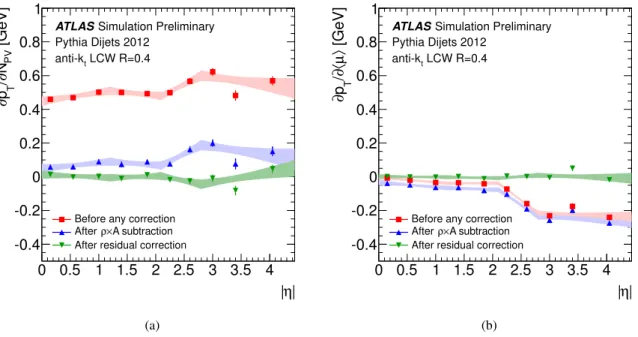
It is observed that after this correction there remains some small dependence of the jet p _T on pile-up, so an additional residual correction is required. This is parameterised in terms of the number of primary vertices, N PV , and the average number of interactions per bunch crossing, hµi, such that both the residual in-time, characterised by N _PV (at fixed hµi), and out-of-time, characterised by hµi (at fixed N _PV ), pile-up dependence can be captured. This is demonstrated in Figure 4 which shows the dependence of the jet p _T on N PV and hµi before and after pile-up correction. The curves in these plots are derived by fitting the dependence on N _PV (hµi) for fixed values of hµi (N PV ), and the gradients for di ff erent fixed hµi (N PV ) are averaged. The calorimeter is designed so that there is some cancellation between in-time and out- of-time pile-up such that when there is an event with unusually high or low N PV with respect to hµi this cancellation will be incomplete and a residual o ff set will remain. This is the e ff ect that dominates in the forward region where we see a substantial dependence on hµi for fixed N PV . This effect is also increased by the application of the area correction. These effects are likely due to the different noise thresholds and granularity of the detector in the forward region and the fact that ρ is derived from the central region of the detector only.

6 Particles with infinitesimal p T .

7 The area here is calculated using a geometric (Voronoi) definition for improved computation speed [35]

η |

| 0 0.5 1 1.5 2 2.5 3 3.5 4 [GeV] PV N ∂ / T p ∂

-0.4 -0.2 0 0.2 0.4 0.6 0.8 1

ATLAS Simulation Preliminary Pythia Dijets 2012

LCW R=0.4 anti-k

Before any correction A subtraction

× After ρ

After residual correction

(a)

η |

| 0 0.5 1 1.5 2 2.5 3 3.5 4 [GeV] 〉 µ〈 ∂ / T p ∂

-0.4 -0.2 0 0.2 0.4 0.6 0.8 1

ATLAS Simulation Preliminary Pythia Dijets 2012

LCW R=0.4 anti-k

Before any correction A subtraction

× After ρ

After residual correction

(b)

Figure 4: Dependence of the reconstructed jet p T on in-time pile-up (a) and out-of-time pile-up (b) at various correction stages in bins of jet |η|. The error bars show the statistical uncertainty on the linear fits to pile-up dependence whilst the band shows the 68% confidence band of a set of 4 linear fits performed on the results in different η regions. Taken from Ref. [36].

The pile-up subtracted p T following area based correction and residual correction, p ^corr _T , is therefore given by:

p ^corr _T = p ^const _T − ρ × A − α × (N PV − 1) − β × hµi (2) where α and β are jet size and algorithm dependent constants derived from Monte Carlo and p ^const _T is the jet p _T at the topo-cluster scale. Ref. [36] gives more details on these corrections. Additionally in Ref. [36]

the systematic uncertainties associated with this correction are discussed. These are parameterised as a function of µ and N _PV , as well as p _T and |η|, and are largest when µ and N _PV deviate from the average conditions in opposite directions.

5.3 Jet Energy Scale

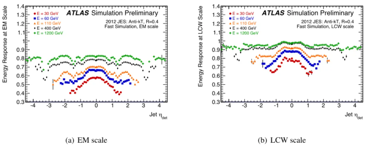
The jet energy scale calibration is derived as a correction which relates the reconstructed jet energy to the truth jet energy [27]. The JES factors are derived from isolated jets (see Section 4.1) from an inclusive jet Monte Carlo sample after the pile-up (Section 5.2) and origin (Section 5.1) corrections have been applied. Figure 5 shows the average energy response which is the inverse of the jet calibration.

Following the calibration in energy it is found that in particular regions of the detector there is a bias in the η distribution with respect to the truth jets. Therefore, an additional correction in purely the angle of the jet is applied to resolve this bias. This also improves the closure in p _T of jets, where the closure in a given quantity is defined by the fit of a Gaussian function to the reconstructed quantity divided by the truth quantity after calibration.

Figure 6 shows the jet E and p _T response plots after the application of the jet energy scale calibration.

It is observed that good closure is demonstrated across the pseudorapidity range. However there is some

small non-closure in low truth jet p _T bins arising from non-gaussian and threshold e ff ects which result

in poor fits at low truth jet p _T .

η

Jet

-4 -3 -2 -1 0 1 2 3 4

Energy Response at EM Scale

0.3 0.4 0.5 0.6 0.7 0.8 0.9 1 1.1 1.2 1.3 1.4

E = 30 GeV E = 60 GeV E = 110 GeV E = 400 GeV E = 1200 GeV

Simulation Preliminary ATLAS

2012 JES: Anti-kT, R=0.4 EM scale

(a) EM scale

η

Jet

-4 -3 -2 -1 0 1 2 3 4

Energy Response at LCW Scale

0.3 0.4 0.5 0.6 0.7 0.8 0.9 1 1.1 1.2 1.3 1.4

E = 30 GeV E = 60 GeV E = 110 GeV E = 400 GeV E = 1200 GeV

Simulation Preliminary ATLAS

2012 JES: Anti-kT, R=0.4 LCW scale

(b) LCW scale

Figure 5: Energy response as a function of η det (the η of the jet relative to the geometric centre of the detector) for EM (a) and LCW (b) scale anti-k t , R = 0.4 jets before calibration.

5.4 Global Sequential Correction

Following the above jet calibration scheme, it is observed that there is a difference between the closure of quark and gluon initiated jets (as defined by angular matching to partons in Monte Carlo) whereby a response di ff erence of up to 8% is observed between quark and gluon initiated jets [37]. This di ff erence previously resulted in one of the largest uncertainties on the jet energy calibration. To reduce the dif- ference between the jet responses of quarks and gluons and thereby improve both jet resolution and jet energy scale uncertainties, further corrections are applied following the JES calibration. These correc- tions include a “punch-through” correction to correct high p _T jets whose energy is not fully contained within the calorimeter jet.

The corrections are applied depending on the topology of energy deposits in the calorimeter, tracking information and muon spectrometer information. Corrections are applied sequentially and in such a way as the mean jet energy response is left unchanged. The five stages correct the jet energy based on (in order):

1. The fraction of energy deposited in the first layer of the tile calorimeter.

2. The fraction of energy deposited in the third layer of the electromagnetic calorimeter.

3. The number of tracks with p _T > 1 GeV associated to the jet.

4. The p _T -weighted transverse width of the jet measured using tracks with p _T > 1 GeV associated to the jet.

5. The amount of activity behind the jet as measured in the muon spectrometer.

Only the track-based and muon spectrometer correction steps are applied to LCW calibrated jets, as calorimeter calibrations have already been included in the local calibration weighting.

Further details and validation of the global sequential correction can be found in Ref. [9].

5.5 Jet Energy Scale in Fast Simulation

The same jet calibration procedure is also used in fast simulation samples using a dedicated set of JES

factors for the calibration in energy and η. Figure 7 shows the energy response as a function of η and

[GeV]

T

p

20 30 10

2 × 10

10

2 × 10

true

E /

E

0.98 0.99 1 1.01 1.02 1.03 1.04 1.05 1.06 1.07 1.08

Fullsim MC JES

Simulation Preliminary ATLAS

Pythia

| < 0.1

| η

, R=0.4, LCW k

anti-

(a) E response vs. p T

det

|

| η

0 0.5 1 1.5 2 2.5 3 3.5 4 4.5

true

E /

E

0.98 0.99 1 1.01 1.02 1.03 1.04 1.05 1.06 1.07 1.08

Fullsim MC JES

Simulation Preliminary ATLAS

Pythia

< 100 GeV p

80 GeV <

, R=0.4, LCW k

anti-

(b) E response vs. | η |

[GeV]

T

p

20 30 10

2 × 10

10

2 × 10

Ttrue

p /

p

0.98 0.99 1 1.01 1.02 1.03 1.04 1.05 1.06 1.07 1.08

Fullsim MC JES

Simulation Preliminary ATLAS

Pythia

| < 0.1

| η

, R=0.4, LCW k

anti-

(c) p T response vs. p T

det

| η

|

0 0.5 1 1.5 2 2.5 3 3.5 4 4.5

Ttrue

p /

p

0.98 0.99 1 1.01 1.02 1.03 1.04 1.05 1.06 1.07 1.08

Fullsim MC JES

Simulation Preliminary ATLAS

Pythia

< 100 GeV p

80 GeV <

, R=0.4, LCW k

anti-

(d) p T response vs. | η |

Figure 6: The energy and p _T response after jet calibration for anti-k t , R = 0.4 jets using LCW topo- clusters. The energy response is shown as a function of p _T for jets in the region |η| < 0.1 (a) and as a function of |η det | (the η of the jet relative to the geometric centre of the detector) for jets in the range 80 < p _T < 100 GeV (b). The p _T response is also shown in the same way (c and d).

Figure 8 shows the jet response after calibration in fast simulation. Comparing these to the full simulation equivalent in Figures 5 and 6 it is observed that the calibration factors in fast simulation are qualitatively different in forward regions, and around 100 GeV there is slightly larger non-closure observed in fast simulation compared to full simulation. The response beyond |η| ∼ 3.2 shows larger discrepancies between full simulation and fast simulation due to the more approximate treatment of the showering of hadrons in the forward calorimeters. This difference is included as an additional fast simulation specific systematic since the in-situ methods are not used to validate fast simulation. The global sequential calibration is not re-derived for the fast simulation calibration but the dependence of the calibration on the variables used is found to be similar.

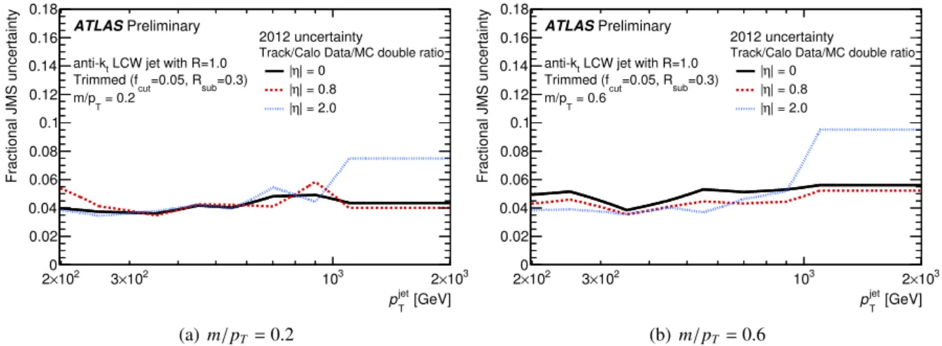
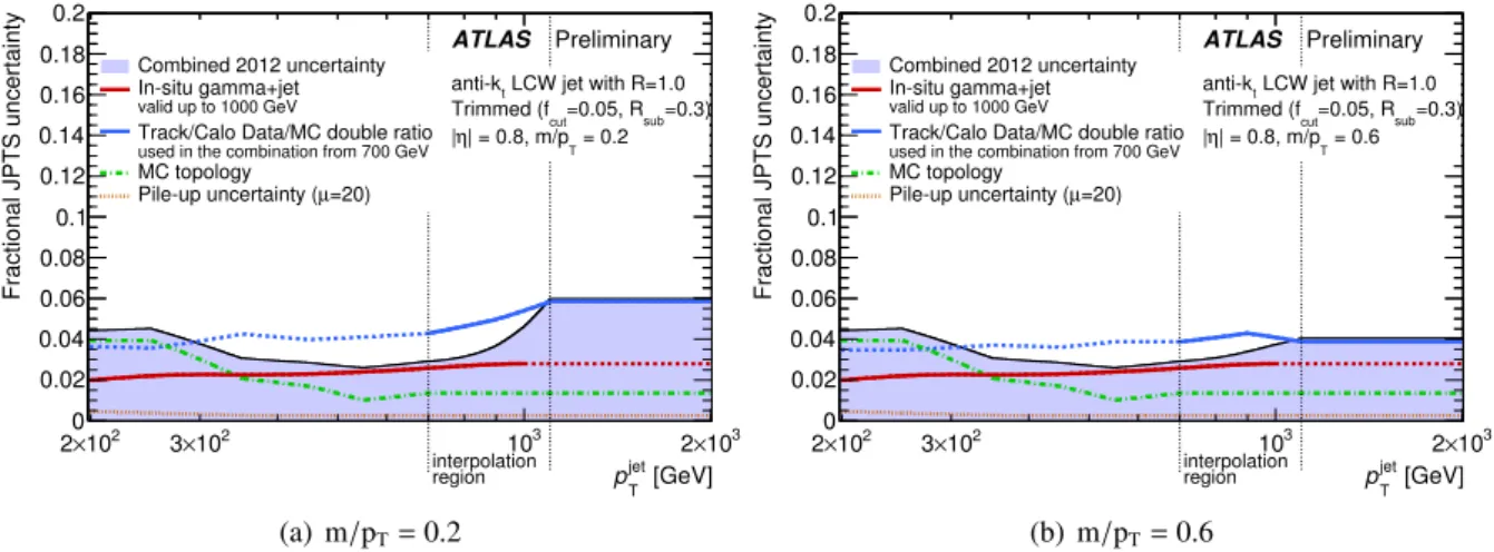
5.6 Jet Energy and Mass Calibration for Large-R Jets

With the high centre-of-mass energy at the LHC, the decay products of highly boosted objects (high p _T relative to their mass) may be fully contained within individual large-radius (large-R) jets. An accurate and precise reconstruction of the jet energy and mass of large-R jets is essential especially in searches for new physics studying the jet invariant mass spectrum [38] or measurements of boosted t¯ t systems [39].

Due to the high-luminosity conditions, soft particles unrelated to the hard scattering contaminate the jets

η

Jet

-4 -3 -2 -1 0 1 2 3 4

Energy Response at EM Scale

0.3 0.4 0.5 0.6 0.7 0.8 0.9 1 1.1 1.2 1.3 1.4

E = 30 GeV E = 60 GeV E = 110 GeV E = 400 GeV E = 1200 GeV

Simulation Preliminary ATLAS

2012 JES: Anti-kT, R=0.4 Fast Simulation, EM scale

(a) EM scale

η

Jet

-4 -3 -2 -1 0 1 2 3 4

Energy Response at LCW Scale

0.3 0.4 0.5 0.6 0.7 0.8 0.9 1 1.1 1.2 1.3 1.4

E = 30 GeV E = 60 GeV E = 110 GeV E = 400 GeV E = 1200 GeV

Simulation Preliminary ATLAS

2012 JES: Anti-kT, R=0.4 Fast Simulation, LCW scale

(b) LCW scale

Figure 7: Energy response as a function of η det (the η of the jet relative to the geometric centre of the detector) for EM (a) and LCW (b) scale anti-k t , R = 0.4 jets in fast simulation before calibration.

in the detector resulting in a degradation of the mass (and energy) resolution of large-R jets. To enhance the sensitivity to new physics processes and to mitigate the influence of pile-up, jet grooming algorithms have been designed. Here a trimming [40] algorithm is used and detailed descriptions and studies of the optimisation of jet grooming algorithm can be found in Refs. [41, 42].

The jet energy and mass scale corrections are derived from a Pythia8 MC sample including pile-up events, as in the standard JES determination procedure (see Section 5.3). The jets are calibrated to truth jets constructed using the same jet algorithm and trimming as in reconstruction. Whereas for the standard jet algorithms (R = 0.4, 0.6) the dependence of the jet response on the number of primary vertices and the average number of interactions is removed by applying a pile–up correction (see Section 5.2), no explicit pile–up correction is applied to large-R jets. Due to the susceptibility to soft, wide-angle contributions which do not significantly impact the jet energy scale, the calibration of the jet mass scale is more challenging. In addition, no origin correction has been applied to large-R jets. Due to the importance in analyses of the mass of large-R jets, following the calibration in energy and η a calibration of the mass of the jets is applied using the same procedure as employed for the energy calibration.

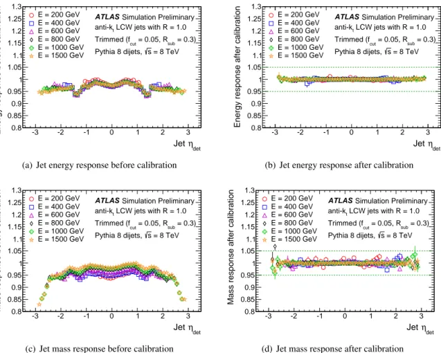
Figure 9 shows the jet energy response as a function of the jet η in different jet energy bins before and after jet energy calibration for anti-k t R = 1.0 trimmed jets. This figure also shows the jet mass response before and after the jet mass calibration which is applied after the jet energy calibration. Prior to calibration, the mean energy and mass scale for low p _T (300 GeV) jets differs up to 10% and 20%, respectively to that of the particle level truth jet quantity whilst higher p _T (1900 GeV) jets di ff er by 5%

and 10% respectively. After the calibration, the detector dependence is reduced and a uniform response across the full energy and η range can be restored. Prior to the correction the mass distribution shows considerable structure due to the position of the di ff erent calorimeter boundaries.

6 In-situ Jet Energy Calibration

Following the MC-based calibration of jets, in-situ techniques employing the balance of physics objects

in the transverse plane, are used in the final stage of the JES calibration. The p _T of reference objects

(photons, Z bosons or other jets) and the jets being calibrated are compared in both data and Monte

[GeV]

T

p

20 30 10

2 × 10

10

2 × 10

true

E /

E

0.98 0.99 1 1.01 1.02 1.03 1.04 1.05 1.06 1.07 1.08

Fastsim MC JES

Simulation Preliminary ATLAS

Pythia

| < 0.1

| η

, R=0.4, LCW k

anti-

(a) E response vs. p T

det

|

| η

0 0.5 1 1.5 2 2.5 3 3.5 4 4.5

true

E /

E

0.98 0.99 1 1.01 1.02 1.03 1.04 1.05 1.06 1.07 1.08

Fastsim MC JES

Simulation Preliminary ATLAS

Pythia

< 100 GeV p

80 GeV <

, R=0.4, LCW k

anti-

(b) E response vs. | η |

[GeV]

T

p

20 30 10

2 × 10

10

2 × 10

Ttrue

p /

p

0.98 0.99 1 1.01 1.02 1.03 1.04 1.05 1.06 1.07 1.08

Fastsim MC JES

Simulation Preliminary ATLAS

Pythia

| < 0.1

| η

, R=0.4, LCW k

anti-

(c) p T response vs. p T

det

| η

|

0 0.5 1 1.5 2 2.5 3 3.5 4 4.5

Ttrue

p /

p

0.98 0.99 1 1.01 1.02 1.03 1.04 1.05 1.06 1.07 1.08

Fastsim MC JES

Simulation Preliminary ATLAS

Pythia

< 100 GeV p

80 GeV <

, R=0.4, LCW k

anti-

(d) p T response vs. | η |

Figure 8: The closure of the jet calibration for anti-k t , R = 0.4 jets using LCW topo-clusters in fast simulation. The energy response is shown as a function of p _T for jets in the region |η| < 0.1 (a) and as a function of |η det | (the η of the jet relative to the geometric centre of the detector) for jets in the range 80 < p _T < 100 GeV (b). The p _T response is also shown in the same way (c and d).

Carlo simulation to measure the ratio

R _data

R _MC = hp ^jet _T /p ^ref _T i _data hp ^jet _T /p ^ref _T i _MC

. (3)

This quantity defines a residual correction which is applied to jets reconstructed in data.

Firstly, dijet events are employed to apply an η-intercalibration in which the average p _T for forward jets (0.8 ≤ |η| < 4.5) is equalised to the p _T of balancing jets in the central region (|η| < 0.8). This intercalibration is documented in Ref. [17] and aims to remove any residual pseudorapidity difference in the jet response following the MC calibration. Note that at low p _T the data is collected using a trigger with a large prescale resulting in larger statistical uncertainties at low p _T .

Figure 10 shows the relative jet response, defined in Equation 3, using a central jet as a reference, of anti-k t , R = 0.4 jets against pseudorapidity, from which the η-intercalibration factors are derived. The η-intercalibration correction factors are generally below 2%.

Following the η-intercalibration, the balance of Z bosons and photons recoiling against jets is used

to derive in-situ JES corrections for jets with |η| < 0.8 as described in Ref. [18]. These measurements are

carried out for jets with 20 ≤ p _T ≤ 200 GeV (Z + jet) and 30 ≤ p _T ≤ 800 GeV (γ + jet).

η det

Jet

-3 -2 -1 0 1 2 3

Energy response before calibration ^0.8 0.85 0.9 0.95 1 1.05 1.1 1.15 1.2 1.25 1.3

E = 200 GeV E = 400 GeV E = 600 GeV E = 800 GeV E = 1000 GeV E = 1500 GeV

ATLAS Simulation Preliminary LCW jets with R = 1.0 anti-k

= 0.3) = 0.05, R

Trimmed (f

= 8 TeV s Pythia 8 dijets,

(a) Jet energy response before calibration

η det

Jet

-3 -2 -1 0 1 2 3

Energy response after calibration _0.8 0.85 0.9 0.95 1 1.05 1.1 1.15 1.2 1.25 1.3

E = 200 GeV E = 400 GeV E = 600 GeV E = 800 GeV E = 1000 GeV E = 1500 GeV

ATLAS Simulation Preliminary LCW jets with R = 1.0 anti-k

= 0.3) = 0.05, R

Trimmed (f

= 8 TeV s Pythia 8 dijets,

(b) Jet energy response after calibration

η det

Jet

-3 -2 -1 0 1 2 3

Mass response before calibration _0.8 0.85 0.9 0.95 1 1.05 1.1 1.15 1.2 1.25 1.3

E = 200 GeV E = 400 GeV E = 600 GeV E = 800 GeV E = 1000 GeV E = 1500 GeV

ATLAS Simulation Preliminary LCW jets with R = 1.0 anti-k

= 0.3) = 0.05, R

Trimmed (f

= 8 TeV s Pythia 8 dijets,

(c) Jet mass response before calibration

η det

Jet

-3 -2 -1 0 1 2 3

Mass response after calibration

0.8 0.85 0.9 0.95 1 1.05 1.1 1.15 1.2 1.25 1.3

E = 200 GeV E = 400 GeV E = 600 GeV E = 800 GeV E = 1000 GeV E = 1500 GeV

ATLAS Simulation Preliminary LCW jets with R = 1.0 anti-k

= 0.3) = 0.05, R

Trimmed (f

= 8 TeV s Pythia 8 dijets,

(d) Jet mass response after calibration

Figure 9: Jet energy response of anti-k t R = 1.0 trimmed jets as a function of the jet η _det (the η of the jet relative to the geometric centre of the detector) before (a) and after (b) the jet energy scale calibration and the jet mass response before (c) and after (d) the jet mass calibration.

Finally, high-p T jets are calibrated using events in which a system of low-p T jets recoil against a single high-p _T jet (multi-jet balance). These studies are documented in Ref. [17]. This requires the low-p T system to be well calibrated and so the method can be iterated starting from jets already well calibrated by other in-situ methods and increasing in p _T until the low number of events prevents accurate calibration. This method covers a range of 300 ≤ p _T ≤ 1700 GeV.

Figure 11 summarises the results of the Z +jet, γ +jet and multi-jet balance analyses showing the ratio of jet response in data and MC. It is observed that across the p _T range from 20-2000 GeV the response agrees in MC and data at the 1% level. The divergence of the response from unity defines the in-situ calibration which is applied to jets in data. Also it can be seen that there is good agreement and little tension between the three different in-situ methods in the regions of phase space where they overlap.

6.1 Combination of In-situ Measurements

The data-to-MC ratio (defined in Equation 3 and shown in Figure 11) from Z + jet, γ + jet and multi-jet

balance are combined using the procedure outlined in Ref. [37]. This combination uses the compatibility

of the three in-situ measurements and their associated systematics to produce a combined measurement

of the response ratio with its associated uncertainty.

η det

− 4 − 3 − 2 − 1 0 1 2 3 4

Data

/ℜ

ℜ

0.9 1 1.1

1.2 Anti-k

R = 0.4, LCW+JES

< 55 GeV

avg

p

≤ 40 GeV

ATLAS Preliminary

= 20 fb

∫ L dt

= 8 TeV Data 2012, s Dijets

-intercalibration η Total uncertainty Statistical component

(a) 40 < p T < 55 GeV

η det

− 4 − 3 − 2 − 1 0 1 2 3 4

Data

/ℜ

ℜ

0.9 1 1.1

1.2 Anti-k

R = 0.4, LCW+JES

< 270 GeV

avg

p

≤ 220 GeV

ATLAS Preliminary

= 20 fb

∫ L dt

= 8 TeV Data 2012, s Dijets

-intercalibration η Total uncertainty Statistical component

(b) 220 < p T < 270 GeV

Figure 10: Relative jet response (see Equation 3) as a function of η det (the η of the jet relative to the geometric centre of the detector) for anti-k t , R = 0.4, LCW jets. The black solid line shows the derived η-intercalibration factors with the bands showing the uncertainty on this correction. The points are the input data to the calibration formed from the ratio of fits to the balance in data and in Monte Carlo. In the central reference region (|η| < 0.8) there is no calibration by construction. p ^avg _T is the average p _T of the two jets in the dijet system.

[GeV]

jet

p

20 30 10

2 × 10

10

2 × 10

0.85

0.9 0.95 1 1.05 1.1

=0.4, EM+JES

t

R anti-k Data 2012

ATLAS Preliminary

|<0.8 η = 8 TeV, | s

∫

L dt = 20 fb

γ +jet Z+jet Multijet Total uncertainty Statistical component

[GeV]

jet

p

20 30 10

2 × 10

10

2 × 10

MC

ℜ /

ℜ

0.85 0.9 0.95 1 1.05 1.1

(a) EM+JES

[GeV]

jet

p

20 30 10

2 × 10

10

2 × 10

0.85

0.9 0.95 1 1.05 1.1

=0.4, LCW+JES

t

R anti-k Data 2012

ATLAS Preliminary

|<0.8 η = 8 TeV, | s

∫

L dt = 20 fb

γ +jet Z+jet Multijet Total uncertainty Statistical component

[GeV]

jet

p

20 30 10

2 × 10

10

2 × 10

MC

ℜ /

ℜ

0.85 0.9 0.95 1 1.05 1.1

(b) LCW+JES

Figure 11: Ratio of response measured in data to response measured in data for Z + jet, γ + jet and multi- jet balance in-situ analyses. Also shown is the combined correction (black line) with its associated uncertainty (green) as discussed in Section 6.1.

The set of 25 uncertainty sources is shown in Table 1 (note that electron and photon energy scales are correlated and therefore counted together) and is separated into four categories:

• Detector description (det.)

• Physics modelling (model)

• Statistics and method (stat. / meth.)

• Mixed detector and modelling (mixed)

where the mixed category contains uncertainties which cannot be fully distinguished as being either a detector or a modelling uncertainty. This separation allows combination of results between experiments as, for example, detector uncertainties are uncorrelated between experiments whilst physics modelling uncertainties are correlated.

The combination is carried out using the in-situ measurements made in bins of p ^ref _T and evaluated at hp ^ref _T i . The data/MC response ratio is defined in fine p ^ref _T bins for each in-situ method using interpolating second order polynomial splines. The combination is then carried out using a weighted average of the in-situ measurements based on a χ ² -minimisation. This local χ ² is also useful to define the level of agreement between in-situ measurements.

Each uncertainty source in the combination is treated as fully correlated across p _T and η and inde- pendent from one another. Each uncertainty is propagated to the combined results using pseudoexper- iments [27]. It may be necessary to understand the contribution of each uncertainty component to the final uncertainty to fully understand any correlations and so, each individual source is propagated sepa- rately to the combined result by coherently shifting all the correction factors by one standard deviation.

Comparison of this shifted combination result to the nominal provides an estimate of the propagated systematic uncertainty.

One exception to this is the flavour uncertainty on the recoil in the multi-jet balance [17]. This is correlated in a non-trivial way to the additional uncertainties considered in analyses due to flavour composition and response. It was found that this did not change the overall in-situ uncertainty after combination with the other in-situ methods by a significant amount and therefore was not included.

To take tensions between measurements into account, each uncertainty source is increased by rescal- ing it by p

χ ² /nd f , where nd f is the number of degrees of freedom, if p

χ ² /nd f is more than 1 [43].

The local p

χ ² /nd f of the final combination is shown in Figure 12. It is observed that p

χ ² /nd f for both jet collections is below 1 for most of the p _T range and never exceeds 2. The combined in-situ factor is used as the final calibration factor to be applied to data after minimising statistical fluctuations using a sliding Gaussian kernel.

[GeV]

jet

p

20 30 40 10

2 × 10

10

/ndf

χ

0 0.5 1 1.5 2 2.5 3 3.5 4

R=0.4, EM+JES anti-k

Data 2012

ATLAS Preliminary = 8 TeV s

∫

L dt = 20 fb

(a) EM + JES

[GeV]

jet

p

20 30 40 10

2 × 10

10

/ndf

χ

0 0.5 1 1.5 2 2.5 3 3.5 4

R=0.4, LCW+JES anti-k

Data 2012

ATLAS Preliminary = 8 TeV s

∫

L dt = 20 fb

(b) LCW + JES

Figure 12: χ ² /nd f for the combination of in-situ measurements. This shows the compatability between the two in-situ methods at each point in the spectra. For a small range we only have one measurement such that there is a gap. The points where the curve touches zero are when the two methods cross.

Figure 13 shows the uncertainty sources for the three in-situ analyses used in the combination as a function of p _T . In the combination, the Z +jet measurement is most important at low p _T , the γ +jet measurement at medium p _T and the multi-jet balance at high p _T .

Figure 11 shows the jet response as a function of jet p _T showing the combined result (black line)

Name Description Category Z + jet

e E-scale material Material uncertainty on electron energy scale det.

e E-scale presampler Presampler uncertainty on electron energy scale det.

e E-scale baseline Baseline uncertainty on electron energy scale mixed e E-scale smearing Uncertainty on electron energy smearing mixed µ E-scale baseline Baseline uncertainty on muon energy scale det.

µ E-scale smearing ID Uncertainty on muon ID momentum smearing det.

µ E-scale smearing MS Uncertainty on muon MS momentum smearing det.

MC generator Difference between MC generators model

JVF JVF choice mixed

∆ φ Extrapolation in ∆ φ model

Out-of-cone Contribution of particles outside the jet cone model Sub-leading jet veto Variation in sub-leading jet veto model

Statistical components Statistical uncertainty stat./meth.

γ + jet

γ E-scale material Material uncertainty on photon energy scale det.

γ E-scale presampler Presampler uncertainty on photon energy scale det.

γ E-scale baseline Baseline uncertainty on photon energy scale det.

γ E-scale smearing Uncertainty on photon energy smearing det.

MC generator Difference between MC generators model

∆ φ Extrapolation in ∆ φ model

Out-of-cone Contribution of particles outside the jet cone model Sub-leading jet veto Variation in sub-leading jet veto model

Photon purity Purity of sample in γ +jets det.

Statistical components Statistical uncertainty stat. / meth.

Multijet balance

α selection Angle between leading jet and recoil system model β selection Angle between leading et and closest sub-leading jet model MC generator Difference between MC generators (fragmentation) mixed p _T asymmetry selection Asymmetry selection between leading and sub-leading jet model

Jet p _T threshold Jet p _T threshold mixed

Statistical components Statistical uncertainty stat./meth.

Table 1: Summary of the uncertainty components propagated through to the combination of in-situ jet

energy scale measurements from Z +jet, γ +jet and multi-jet balance studies. These are discussed in more

detail in Refs. [17, 18].

and its associated statistical (blue) and total (green) uncertainties. A general offset of 0.5% is observed between the data and MC (with data below MC). The uncertainty from the combination of in-situ tech- niques is about 2.5% (3.5%) at low p _T (25 GeV) for EM (LCW) jets and decreases to about 1% (1%) at higher p _T (above 200 GeV).

[GeV]

jet

p

20 30 10

2 × 10

10

2 × 10

Relative uncertainties

0 0.005 0.01 0.015 0.02 0.025

=0.4, EM+JES

t

R anti-k Data 2012

ATLAS Preliminary

|<0.8 η = 8 TeV, |

∫ s

L dt = 20 fb φ cut

∆

-scale material E

e E -scale presampler e

-scale baseline e E

-scale smearing e E

MC generator JVF E -scale baseline µ

-scale smearing ID µ E

-scale smearing MS µ E

Out-of-cone Subleading jet veto Statistical components Z+jet

(a) Z + jets (EM + JES)

[GeV]

jet

p

20 30 10

2 × 10

10

2 × 10

Relative uncertainties

0 0.005 0.01 0.015 0.02 0.025

=0.4, LCW+JES

t

R anti-k Data 2012

ATLAS Preliminary

|<0.8 η = 8 TeV, |

∫ s

L dt = 20 fb φ cut

∆

-scale material E

e E -scale presampler e

-scale baseline e E

-scale smearing e E

MC generator JVF E -scale baseline µ

-scale smearing ID µ E

-scale smearing MS µ E

Out-of-cone Subleading jet veto Statistical components Z+jet

(b) Z + jets (LCW + JES)

[GeV]

jet

p

20 30 10

2 × 10

10

2 × 10

Relative uncertainties

0 0.005 0.01 0.015 0.02 0.025

=0.4, EM+JES

t

R anti-k Data 2012

ATLAS Preliminary

|<0.8 η = 8 TeV, | s

∫

L dt = 20 fb φ cut

∆

MC generator -scale material Photon E

-scale presampler Photon E

-scale baseline Photon E

-scale smearing Photon E

Photon purity Out-of-cone Subleading jet veto Statistical components γ +jet

(c) γ+jets (EM+JES)

[GeV]

jet

p

20 30 10

2 × 10

10

2 × 10

Relative uncertainties

0 0.005 0.01 0.015 0.02 0.025

=0.4, LCW+JES

t

R anti-k Data 2012

ATLAS Preliminary

|<0.8 η = 8 TeV, | s

∫

L dt = 20 fb φ cut

∆

MC generator -scale material Photon E

-scale presampler Photon E

-scale baseline Photon E

-scale smearing Photon E

Photon purity Out-of-cone Subleading jet veto Statistical components γ +jet

(d) γ+jets (LCW+JES)

[GeV]

jet

p

20 30 10

2 × 10

10

2 × 10

Relative uncertainties

0 0.005 0.01 0.015 0.02 0.025

=0.4, EM+JES

t

R anti-k Data 2012

ATLAS Preliminary

|<0.8 η = 8 TeV, | s

∫

L dt = 20 fb selection

α selection β

MC generator asymmetry selection p

threshold Jet p

Statistical components Multijet

(e) Multi-jet balance (EM+JES)

[GeV]

jet

p

20 30 10

2 × 10

10

2 × 10

Relative uncertainties

0 0.005 0.01 0.015 0.02 0.025

=0.4, LCW+JES

t

R anti-k Data 2012

ATLAS Preliminary

|<0.8 η = 8 TeV, | s

∫

L dt = 20 fb selection

α selection β

MC generator asymmetry selection p

threshold Jet p

Statistical components Multijet

(f) Multi-jet balance (LCW+JES)

Figure 13: Individual uncertainty sources used in the combination for the three in-situ calibration meth-

ods. The systematic uncertainties displayed correspond to those in Table 1.

6.2 Single Hadron Response

Such in-situ methods as detailed above can also be compared to a method whereby the jet energy scale is estimated from the response of single hadrons. This firstly provides a cross check of the direct balance in-situ methods described above, albeit with a larger uncertainty and also allows the extension of in-situ measurements of the jet energy scale to higher energies which the direct balance methods are unable to reach due to limited data. Jets are treated as a superposition of the individual energy deposits of their constituent particles as described in Refs. [44, 45].

In Ref. [37] the in-situ methods described above and the single hadron response studies are seen to be in agreement, both showing an approximate 2% shift between the jet energy scale in data and Monte Carlo. However the other in-situ methods show a considerably smaller uncertainty (approximately 2%

compared to 5%) and so the single particle response method is only used at high p _T (> 1500 GeV) where the statistical power of in-situ methods becomes limited. The single hadron response measurements from 2011 data-taking are propagated to high p _T jets to provide an uncertainty beyond the reach of the in-situ analyses described previously.

This uncertainty is determined by propagating the energy response uncertainty of all particles con- tributing to a jet. For charged hadron momenta below 20 GeV, the single charged hadron response is used, while for higher momenta, the response measured in the ATLAS combined test beam is included.

For the response to neutral pions, the uncertainty on the electromagnetic calorimeter energy scale is dominant, while for all other neutral hadrons an additional uncertainty due to the limited knowledge of the calorimeter hadron response.

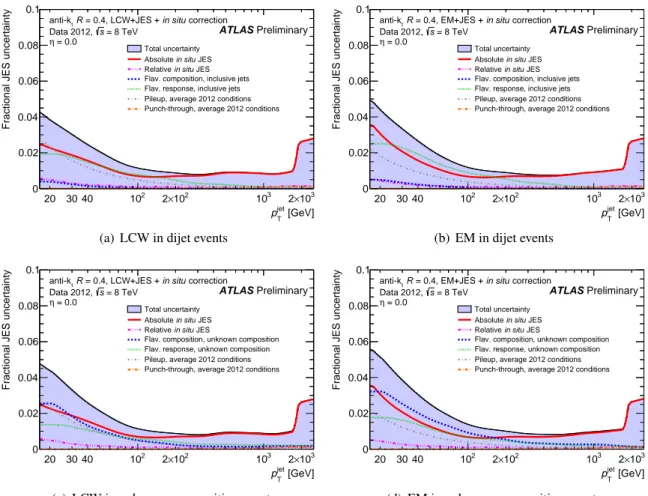
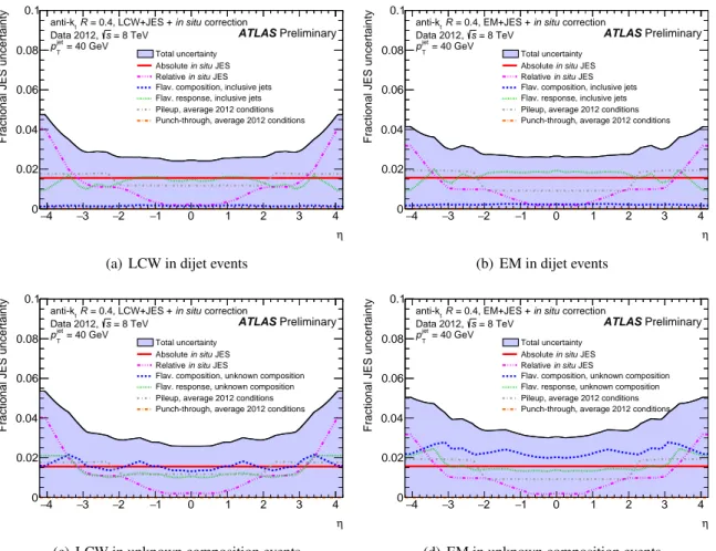
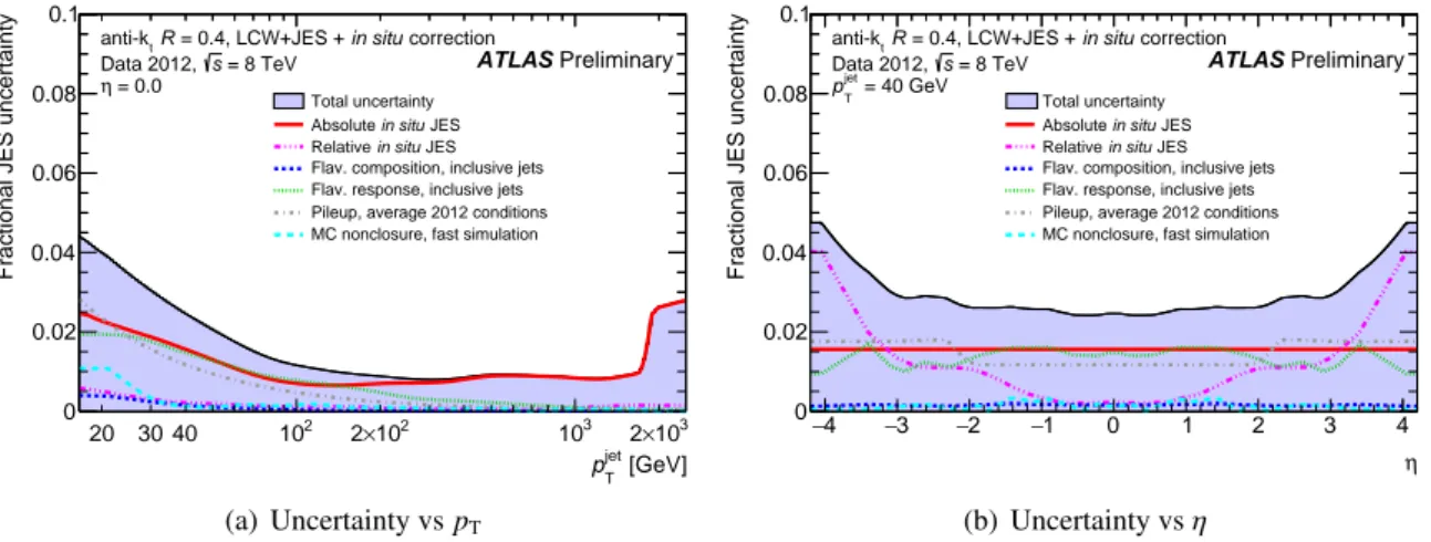
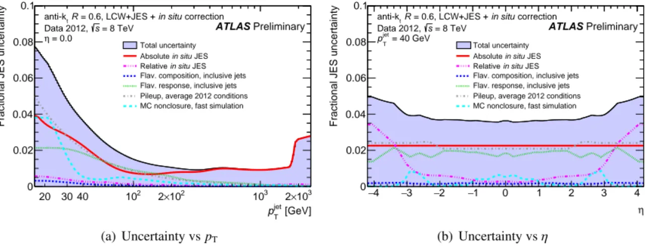
7 Jet Energy Scale Uncertainties

The total jet energy scale uncertainty is compiled from multiple sources:

1. 22 systematic sources from in-situ methods as discussed above 2. 34 statistical sources from in-situ methods as discussed above

3. a single-hadron response uncertainty which only a ff ects the highest p _T jets beyond the reach of in-situ techniques.

4. 2 (one systematic, one statistical) η-intercalibration uncertainties

5. 4 sources from uncertainties associated to the pile-up corrections as outlined in Ref. [36]:

• µ dependent uncertainty on the pile-up correction

• N _PV dependent uncertainty on the pile-up correction

• p _T dependence of pile-up corrections

• ρ mis-modelling

6. 2 sources due to jet flavour as discussed below

These terms are assumed to be independent and result in a jet energy scale uncertainty defined in terms of

65 parameters (nuisance parameters). The total jet energy scale uncertainty resulting from this is shown

in Figures 14 and 15.

[GeV]

jet

p T

20 30 40 10 ² 2 × 10 ² 10 ³ 2 × 10 ³

Fractional JES uncertainty

0 0.02 0.04 0.06 0.08 0.1

ATLAS Preliminary correction

in situ = 0.4, LCW+JES +

t

R anti-k

= 8 TeV s Data 2012,

= 0.0

η Total uncertainty

JES

Absolute

JES

Relative

Flav. composition, inclusive jets Flav. response, inclusive jets Pileup, average 2012 conditions Punch-through, average 2012 conditions

(a) LCW in dijet events

[GeV]

jet

p T

20 30 40 10 ² 2 × 10 ² 10 ³ 2 × 10 ³

Fractional JES uncertainty

0 0.02 0.04 0.06 0.08 0.1

ATLAS Preliminary correction

in situ = 0.4, EM+JES +

t

R anti-k

= 8 TeV s Data 2012,

= 0.0

η Total uncertainty

JES

Absolute

JES

Relative

Flav. composition, inclusive jets Flav. response, inclusive jets Pileup, average 2012 conditions Punch-through, average 2012 conditions

(b) EM in dijet events

[GeV]

jet

p T

20 30 40 10 ² 2 × 10 ² 10 ³ 2 × 10 ³

Fractional JES uncertainty

0 0.02 0.04 0.06 0.08 0.1

ATLAS Preliminary correction

in situ = 0.4, LCW+JES +

t

R anti-k

= 8 TeV s Data 2012,

= 0.0

η Total uncertainty

JES

Absolute

JES

Relative

Flav. composition, unknown composition Flav. response, unknown composition Pileup, average 2012 conditions Punch-through, average 2012 conditions

(c) LCW in unknown composition events

[GeV]

jet

p T

20 30 40 10 ² 2 × 10 ² 10 ³ 2 × 10 ³

Fractional JES uncertainty

0 0.02 0.04 0.06 0.08 0.1

ATLAS Preliminary correction

in situ = 0.4, EM+JES +

t

R anti-k

= 8 TeV s Data 2012,

= 0.0

η Total uncertainty

JES

Absolute

JES

Relative

Flav. composition, unknown composition Flav. response, unknown composition Pileup, average 2012 conditions Punch-through, average 2012 conditions

(d) EM in unknown composition events

Figure 14: The total jet energy scale uncertainty as a function of p T for central jets. Two flavour com-

positions are shown, that for dijet events, where the quark / gluon composition is taken from Monte Carlo

and an associated uncertainty from generator comparisons, and that for an unknown flavour composi-

tion (assuming 50:50 quark:gluon jets with a 100% uncertainty). “Absolute in situ JES” refers to the

uncertainty arising from V + jet and multi-jet measurements whilst “Relative in situ JES” refers to the

uncertainty arising from the dijet η-intercalibration. “Punch-through” refers to the uncertainty on the

final (muon-based) stage of the global sequential correction.