In situ jet pseudorapidity intercalibration of the ATLAS detector using dijet events in √

(1)

ATLAS-CONF-2012-124 27August2012

ATLAS NOTE

ATLAS-CONF-2012-124

August 26, 2012

In situ jet pseudorapidity intercalibration of the ATLAS detector using dijet events in √

s = 7 TeV proton-proton 2011 data

The ATLAS Collaboration

Abstract

The response of the ATLAS calorimeters to jets is studied by evaluating the balance between the transverse momenta of the two jets in di-jet events in proton-proton collisions at

√

s =

7 TeV using a dataset corresponding to an integrated luminosity of 4.5 fb

⁻¹

. The results indicate that the pseudorapidity dependence of the jet response is understood for high

p_T

jets across the full calorimeter range. A calibration is derived to correct the jets in data for residual e

ff

ects not captured by the inital Monte Carlo derived calibration. For jets with

p_T >

40 GeV, the uncertainty on this calibration is less than 1% for all jets with

|η_det|<

1.0 and less than 2.5% for jets with

|η_det|<

2.8. The uncertainty is largest for low

p_T

jets in the very forward region

|η_det|>

3.2, where it can be as large as 5.5%.

c

Reproduction of this article or parts of it is allowed as specified in the CC-BY-3.0 license.

(2)

1 Introduction

The jet response of the ATLAS calorimeters depends on the jet’s energy and direction, primarily due to: the non-compensating nature of the ATLAS calorimeters; the use of different detector technologies;

and, the varying amount of dead material in front of the calorimeters. A calibration is therefore needed to ensure a uniform calorimeter response to jets. For the ATLAS detector, this is achieved by applying correction factors derived from Monte Carlo (MC) simulations [1]. For the 2010 dataset, with an inte- grated luminosity of 38 pb

⁻¹

, the uncertainty of this MC-derived calibration was estimated using single hadron response measurements [2], systematic variations of Monte Carlo simulations, and various in situ techniques comparing the jet transverse momentum ( p

_T

) to that of a reference object. Several such in situ studies were performed exploiting the transverse momentum balance in dijet, Z

+jet and

γ

+jet events, as

well as using tracks matched to jets [1]. The jet calibration uncertainty was estimated to about 2.5%

in the central calorimeter region over a wide momentum range of 60

.

p

_T

< 800 GeV. In the forward region (|η| > 2)

¹

, the uncertainty was about 4% for jets with p

_T

> 50 GeV, rising to approximately 12%

for jets with η

≈

4 and p

_T ≈

25 GeV.

The larger ATLAS 2011 dataset makes it possible to further improve the precision of the jet energy measurement. This is achieved by deriving a residual calibration to the jets based on detailed comparisons of data and Monte Carlo simulation using in situ techniques. In this note, the relative jet calorimeter response is measured by balancing the transverse momenta of dijets. This is an update of two earlier analyses [3] that were based on early and late 2010 datasets. The major difference with respect to the previous analyses is that this note presents a measurement of a residual calibration and its uncertainty, while the previous studies estimated an uncertainty by comparing data to MC. The event selection is also altered to account for the 2011 data taking conditions (pileup) and the new jet triggers.

2 The ATLAS detector

The ATLAS detector is described in detail in [4]. In this analysis, the tracking detectors are used to identify primary collision vertices, and to judge if sub-leading jets originate from the hard scatter vertex or from any additional primary vertex produced by pileup interactions. The calorimeters are used to reconstruct jets.

The Inner Detector consists of layers of silicon pixel detectors, silicon microstrip detectors and transi- tion radiation tracking detectors, all of which are immersed in a solenoid magnet that provides a uniform magnetic field of 2 T. The Inner Detector has complete azimuthal coverage and spans the region

|η|

< 2.5.

The electromagnetic calorimetry is provided by high granularity liquid argon (LAr) sampling calorime- ters using lead as an absorber that are split into barrel (|η| < 1.475) and end-cap (1.375 <

|η|

< 3.2) regions. The hadronic calorimeter is divided into four regions. The barrel region (

|η|

< 0.8) and the ex- tended barrel region (0.8 <

|η|

< 1.7) are both instrumented with a tile scintillator/steel calorimeter. The Hadronic End-Cap region (1.5 <

|η|

< 3.2) uses LAr

/

copper calorimeter modules. Finally, the Forward Calorimeter region (3.1 <

|η|

< 4.9) is instrumented with LAr

/

copper and LAr

/

tungsten modules that provide electromagnetic and hadronic energy measurements, respectively.

1The coordinate system used by ATLAS is a right-handed Cartesian coordinate system. The positivez-direction is defined as the direction of the anti-clockwise beam. Pseudorapidity is defined asη=−ln tan(θ/2), whereθis the angle with respect to thez-axis. The azimuthal angle in the transverse planeφis defined to be zero along thex-axis, which points toward the center of the LHC ring.

(3)

3 Data and simulated samples

The data sample considered in this note has been collected using the ATLAS single jet triggers between April and October of 2011. All ATLAS sub-detectors were required to be operational, and the dataset corresponds to a total integrated luminosity of 4.5 fb

⁻¹

of proton-proton collisions at

√

s

=

7 TeV.

Protons are organized in bunch trains with each train having

≈

30 bunches separated by 50 ns. The LHC instantaneous luminosity rose through the data taking period, with two distinct periods of smoothly rising luminosity. The first sub-set of the recorded data constitutes a relatively low pileup sample with an average number of interactions per bunch crossing (µ) between 3 and 8 (average of about 6), while the second sub-set is a higher pileup sample with µ between 5 and 17 (average of about 12).

The dijet baseline simulation samples are produced with the leading order event generator Pythia [5], version 6.423, which uses p

_T

-ordered parton showers to model additional radiation [6]. P

ythia

is used with the modified leading-order parton distribution function (PDF) set MRST LO* [7], and with the ATLAS MC11 AUET2B MRST LO** tune.

The H

erwig++

[8] event generator, version 2.5.2, is used to produce samples for comparison and evaluation of systematic uncertainties. H

erwig++

uses angular-ordered parton showers in the leading- logarithm approximation [9,

10], and the underlying event and soft inclusive interactions are described

using a hard and soft multiple partonic interactions model [11]. The ATLAS MC11 AUET2 LO**

tune [12] with the MRST LO* PDF set [7] is used in the production of the H

erwig++

samples.

The pileup is modelled using simulated minimum bias events generated using Pythia8 [13] with the 4C tune and MRST LO** PDF. These events are overlaid onto the hard scattering events following a Poisson distribution around the average number of additional pp collisions per bunch crossing, µ. The effects from pileup events occurring in nearby bunch crossings (out-of-time pileup) are also modelled by overlaying the hard scattering event with simulated detector signals from P

ythia

8 minimum bias events.

These overlaid events are sampled from out-of-time bunches according to a simulation of the LHC bunch train structure.

4 Jet reconstruction and calibration

Jets are reconstructed using the anti-k

t

algorithm [14] with distance parameters R

=

0.4 and R

=

0.6 using the F

ast

J

et

software [15]. The inputs to the jet algorithm are stable simulated particles (truth jets) or energy deposits in the calorimeter.

The jets used in this analysis (calorimeter jets) are built from topological calorimeter clusters (topo- clusters) [1,

16,17]. Jets are reconstructed separately from topo-clusters at the electromagnetic (EM)

scale

²

, as well as on the local cluster weighting (LCW) scale [?]. The LCW calibration method classifies each topo-cluster as either electromagnetic or hadronic. Based on this classification, a dedicated cor- rection is applied that corrects for the effects of non-compensation, signal losses due to noise threshold e

ff

ects, and energy lost in non-instrumented regions. The LCW calibration is derived from single pion Monte Carlo simulations.

The jets at EM and LCW scale are further calibrated in three subsequent steps. First, the dependence on the jet response from the number of primary vertices N

_PV

and the average number of interactions µ is removed by applying a pileup correction derived from simulated samples [?]. Second, a jet origin correction [1] is applied adjusting the direction of the jet such that it points back to the primary vertex with the highest

P

tracks

p

²_T

. Finally, an energy and pseudorapidity dependent correction [1] is applied that was derived from a MC sample that includes pileup events. The full calibration schemes that include the pileup and MC-derived jet energy scale (JES) corrections are referred to as EM+JES and LCW+JES.

2The electromagnetic scale is the basic calorimeter signal scale for the ATLAS calorimeters. It gives the correct response for the energy deposited in electromagnetic showers, while it does not correct for the lower hadron response.

(4)

5 Intercalibration using events with dijet topologies

5.1 Intercalibration using a central reference region

The standard approach for η intercalibration with dijet events [4] is to use the central region of the calorimeters as the reference region. The relative calorimeter response of jets in other calorimeter re- gions is quantified by the p

_T

balance between the reference jet and the probe jet, exploiting the fact that these jets are expected to have equal p

_T

due to transverse momentum conservation. The p

_T

balance is characterized by the asymmetry

A, defined as

A=

p

^probe_T −

p

^ref_T

p

^avg_T

, (1)

with p

^avg_T =

( p

^probe_T +

p

^ref_T

)/2. The reference region is chosen as the central region of the barrel calorimeter:

|η|

< 0.8. If both jets fall into the reference region, each jet is used, in turn, to probe the other. As a consequence, the average asymmetry in the reference region will be zero by construction.

The asymmetry is then used to measure an η-intercalibration factor c of the probe jet, or its response relative to the reference jet 1/c, using the relation

p

^probe_T

p

^ref_T =

2

+A

2

−A =

1/c. (2)

The analysis is performed in bins of jet η

_det

and p

^avg_T

, where η

_det

is defined as the jet η with respect to the detector position, not taking into account the primary vertex position. Using the standard method outlined above, there is an asymmetry distribution

A_ik

for each probe jet η

det

-bin i and each p

^avg_T

-bin k (an overview of the binning is given in Figure

1). Intercalibration factors are calculated for each bin

according to Equation (2), resulting in

c

_ik=

2

− hAiki

2

+hA_iki

, (3)

where the

hA_iki

is the mean value of the asymmetry distribution in each bin. The uncertainty on

hA_iki

is taken to be the RMS

/√

N of each distribution. For the data, N is the number of events in the bin, while for the MC sample, N is the number of effective events calculated using the MC event weights

³

. The above procedure will hereafter be referred to as the central reference method.

5.2 Intercalibration using the matrix method

A disadvantage with the method outlined above is that all events are required to have a jet in the central reference region. This results in a significant loss of event statistics, especially in the forward region, where the dijet cross section drops steeply as the rapidity interval between the jets increases. In order to use the full statistics, one can extend the default method by replacing the “probe” and “reference” jets by

“left” and “right” jets defined from η

^left

< η

^right

. Equations (1) and (2) then become:

A=

p

^left_T −

p

^right_T

p

^avg_T

, and

R=

p

^left_T

p

^right_T =

c

^right

c

^left =

2

+A

2

−A

, (4)

where the term

R

denotes the ratio of the responses, and c

^left

and c

^right

are the η-intercalibration factors for the left and right jets, respectively.

3The number of effective events is calculated asN_eff =(Pwi)²/Pw²_i, where the sum is over all events, andwiis the event weight for eventi.

(5)

In this approach there is a response ratio distribution,

Ri jk

, whose average value

D

R

i jk

E

is evaluated for each η

^left

-bin i, η

^right

-bin j and p

^avg_T

-bin k. The relative correction factor c

_ik

for given jet η-bin i and for a fixed p

^avg_T

-bin k, is obtained by minimizing a matrix of linear equations:

S (c

_1k

, ..., c

Nk

)

=

N

X

j=1 j−1

X

i=1







1

∆D R_{i jk}E

c

ik

DR_{i jk}E

−

c

jk







2

+

X(c

_1k

, ..., c

Nk

), (5)

where N are the number of η-bins,

∆hRi

is the statistical uncertainty of

hRi

and the function X(c

ik

) is used to quadratically suppress deviations from unity of the average corrections

⁴

. The minimization (Eq.

5) is done separately for each

p

_T

-bin k, and the resulting calibration factors c

_i

(for each jet η-bin i) are scaled such that the average calibration factor in the reference region

|η_det|

< 0.8 equals unity.

6 Event selection

6.1 Trigger selection

Events were retained from the calorimeter trigger stream using a combination of central (

|η_det|

< 3.2) and forward (|η

_det|

> 3.1) jet triggers. The selection was designed such that the trigger efficiency, for a specific region of p

^avg_T

, was greater than 99% and approximately flat as a function of the pseudorapidity of the probe jet. Due to the different prescales for the central and forward jet triggers the data collected by each trigger will correspond to different integrated luminosities. To correctly normalize the data, events were assigned weights depending on the luminosity and the trigger decisions according to the exclusion method, described in Reference [18].

6.2 Data and jet quality selection

All ATLAS sub-detectors were required to be operational and events were rejected if any data quality issues were present. The leading two jets were required to fulfil the default set of jet quality criteria [1].

A dead calorimeter region was present for a subset of the data. To remove any bias from this region, events were removed if any jets were reconstructed close to this region.

6.3 Dijet topology selection

In order to use the momentum balance of dijet events to measure the jet response, it is important that the events used have a 2

→

2 topology. If a third jet is produced in the same pp interaction, the balance between the leading two jets is influenced. In order to judge whether a jet originates from the hard scattering vertex or an additional interaction, a quantity labelled jet vertex fraction (JVF) is computed.

For a given jet, all charged tracks matched to the jet that originate from any primary vertex are selected.

The JVF variable is defined as the track p

_T

sum of those associated with the hard scattering vertex divided by the p

_T

sum of all these tracks. Any jet that has

|η_det|

< 2.5 and JVF > 0.6 is classified as ”vertex confirmed” (j

^central_sub

) since it is likely to originate from the hard scattering vertex. To increase the number of events that have a 2

→

2 topology, selection criteria on the azimuthal angle between the two leading jets

∆

φ(j

₁

, j

2

) and p

_T

requirements on additional jets were applied. Table

1

summarizes the topology selection criteria.

4X(c1k, ...,cNk) = K

N_bins⁻¹ PN_bins i=1 cik−12

, withKbeing a constant andNbinsbeing the number of η-bins (number of in- dicesi). This term prevents the minimization from choosing the trivial solution: allcikequal to zero. The value of the constant Kdoes not influence the solution as long as it is sufficiently large (K≈Nbinsor larger).

(6)

Variable Selection

∆

φ(j

₁

, j

₂

) > 2.5 rad

p

_T

(j

^central_sub

) < max( 0.25 p

^avg_T

, 12 GeV ) p

_T

(j

^fwd_sub

) < max( 0.20 p

^avg_T

, 10 GeV ) JVF(j

^central_sub

) > 0.6

Table 1: Summary of the event topology selection criteria applied in this analysis. Here j

^central_sub

denotes the highest p

_T

sub-leading jet with

|η_det|

< 2.5 and jet vertex fraction (JVF) greater than 60%, and j

^fwd_sub

is the highest p

_T

sub-leading jet with

|η_det|

> 2.5. Sub-leading refers to any jet other than the leading two jets that are used in the measurements.

[GeV]

jet pT

20 30 40 10² 2×10² 10³

detηjet

-4 -2 0 2

4 ATLAS Preliminary

= 0.4, EM+JES

tR Anti-k

(a)

[GeV]

jet pT

30 40 10² 2×10² 10³

detηjet

-4 -2 0 2

4 ATLAS Preliminary

= 0.6, EM+JES

tR Anti-k

(b)

Figure 1: Overview of the ( p

^avg_T

, η

det

)-bins of the dijet balance measurements for jets reconstructed with distance parameter R

=

0.4 and R

=

0.6 calibrated using the EM

+

JES scheme. The solid lines indicate the ( p

^avg_T

, η

_probe

) bin-edges, and the points show the average transverse momentum and pseudorapidity of the probe jet within each bin. The measurements within the η

det

-range spanned by the two thick, dashed lines are used to derive the residual calibration.

This selection differs from that used in previous studies [3] due to the much higher instantaneous luminosities experienced during data taking. The vertex confirmation is applied to make sure that the sub- leading jet considered in the selection originated from the hard scattering vertex. In the forward region

|η_det|

> 2.5, no tracking is available, and events containing any additional forward jet with significant p

_T

are removed (see the criteria above).

7 Dijet balance results

7.1 Binning of the balance measurements

An overview of the ( p

^avg_T

, η

_det

)-bins used in the analysis is presented in Figure

1. All events falling in a

given p

^avg_T

-bin are collected using a dedicated central and forward trigger combination. The statistics in each p

_T

-bin are similar, except for the highest p

^avg_T

-bins that have fewer events. The statistical precision of the measurements is also worse for the low p

^avg_T

-bins as the event selection rejects more events (larger sensitivity to pileup) and due to the wider asymmetry distributions because of the worse jet resolution.

Each p

^avg_T

-bin is further divided into several η-bins. The η-binning is motivated by detector geometry

and statistics.

(7)

cRelative jet response, 1/

0.9 1 1.1

1.2 Anti-k_tR = 0.4, EM+JES < 55 GeV

avg

pT

≤ 40

ATLAS Preliminary Central reference method

Data Pythia

Matrix method

Data Pythia

ηdet

-4 -3 -2 -1 0 1 2 3 4

MC / data 0.9

0.95 1 1.05

(a)

0.9 1 1.1

avg

pT

≤ 220

ATLAS Preliminary Central reference method

Data Pythia

Matrix method

Data Pythia

ηdet

-4 -3 -2 -1 0 1 2 3 4

MC / data 0.9

0.95 1 1.05

(b)

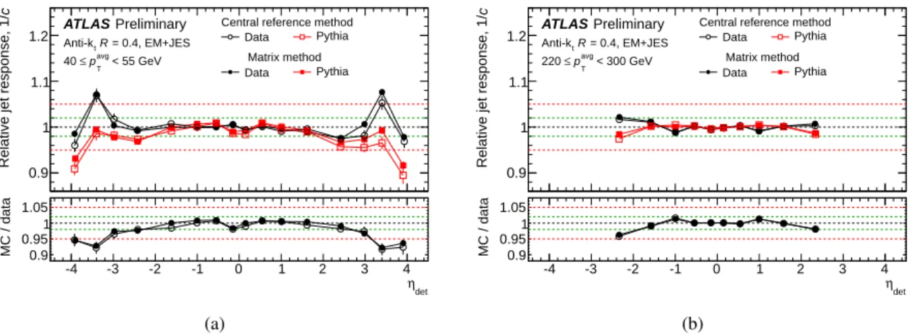
Figure 2: Relative response for anti-k

t

jets with R

=

0.4 calibrated with the EM+JES scheme as a function of the probe jet pseudorapidity measured using the matrix and the central reference methods.

Results are presented for two bins of p

^avg_T

: 40

≤

p

^avg_T

< 55 GeV and 220

≤

p

^avg_T

< 300 GeV.

7.2 Comparison of intercalibration methods

In this section, the relative jet response obtained with the matrix method is compared to the relative jet response obtained using the central reference method. Figures

2a and2b show the jet response relative

to central jets (1/c) for two p

^avg_T

-bins: 40

≤

p

^avg_T

< 55 GeV and 220

≤

p

^avg_T

< 300 GeV. In the most forward region at low p

_T

, the matrix method tends to give a slightly higher relative response compared to the central reference method (see Figure

2a). However the same relative shift is observed both for data

and MC, and consequently the data over MC ratios are consistent. The matrix method is therefore used to measure the relative response as it has better statistical precision.

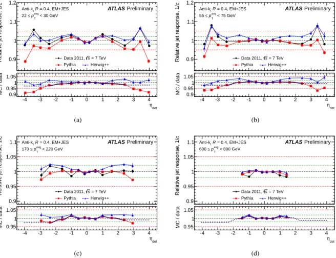
7.3 Comparison of data with Monte Carlo simulation

Figure

3

shows the relative response obtained using the matrix method as a function of the jet pseudora- pidity for data and the Monte Carlo event generator simulations. Four different p

^avg_T

regions are shown:

22

≤

p

^avg_T

< 30 GeV, 55

≤

p

^avg_T

< 75 GeV, 170

≤

p

^avg_T

< 220 GeV and 600

≤

p

^avg_T

< 800 GeV.

Figure

4

shows the relative response as a function of p

^avg_T

for two representative η

_det

-bins, namely

−

1.2

≤

η

_det

<

−

0.8 and 2.1

≤

η

_det

< 2.8. The general features of the response in data are reasonably well reproduced by the Monte Carlo simulations. However, just as observed in the previous studies [3], the H

erwig++

MC predicts a higher relative response than P

ythia

for jets outside the reference region (

|η_det|

> 0.8). Data tend to fall in-between the two predictions. This discrepancy has been investigated and is observed both for truth jets built from stable particles (before any detector modelling), and also jets built from partons (before hadronization). The di

ff

erences therefore reflect a di

ff

erence in physics modelling between the event generators, most likely due to the parton showering. The Pythia predic- tions are based upon a p

_T

-ordered parton shower whereas the H

erwig++

predictions are based on an angular-ordered parton shower.

For p

_T

> 40 GeV and

|η_det|

< 2, Pythia tends to agree better with data than Herwig++ does. In

the more forward region, the spread between the P

ythia

and H

erwig++

response predictions increases

and reaches approximately 5% at

|η_det|=

4. In the most forward region (|η

_det|

> 3) the relative response

prediction of Herwig++ generally agrees better with data than Pythia.

(8)

cRelative jet response, 1/ 0.9

1 1.1 1.2

= 0.4, EM+JES

tR Anti-k

< 30 GeV

avg

pT

≤ 22

ATLAS Preliminary

= 7 TeV s Data 2011, Pythia Herwig++

ηdet

-4 -3 -2 -1 0 1 2 3 4

MC / data 0.9

0.95 1 1.05

(a)

1 1.1 1.2

= 0.4, EM+JES

tR Anti-k

< 75 GeV

avg

pT

≤ 55

ηdet

-4 -3 -2 -1 0 1 2 3 4

MC / data 0.9

0.95 1 1.05

(b)

0.9 0.95 1 1.05

avg

pT

≤ 170

ηdet

-4 -3 -2 -1 0 1 2 3 4

MC / data 0.95 1 1.05

(c)

0.9 0.95 1 1.05

avg

pT

≤ 600

ηdet

-4 -3 -2 -1 0 1 2 3 4

MC / data 0.95 1 1.05

(d)

Figure 3: Relative jet response, 1/c, as a function of the jet pseudorapidity for anti-k

t

jets with R

=

0.4 calibrated with the EM+JES scheme, separately for 22 < p

^avg_T

< 30 GeV, 55 < p

^avg_T

< 75 GeV, 170 <

p

^avg_T

< 220 GeV and 600 < p

^avg_T

< 800 GeV. The lower parts of the figures show the ratios between the data and MC relative response. These measurements were performed using the matrix method.

0.9 0.95 1 1.05

1.1 Anti-k_tR = 0.4, EM+JES < -0.8 ηdet

≤ -1.2

[GeV]

avg

pT

30 40 50 10² 2×10² 10³

MC / data 0.95 1 1.05

(a)

0.9 0.95 1 1.05

1.1 Anti-k_tR = 0.4, EM+JES < 2.8 ηdet

≤ 2.1

[GeV]

avg

pT

30 40 50 10² 2×10² 10³

MC / data 0.95 1 1.05

(b)

Figure 4: Relative jet response, 1/c, as a function of the jet p

_T

for anti-k

t

jets with R

=

0.4 calibrated

with the EM+JES scheme, separately for

−1.2 ≤

η

_det

<

−0.8 and 2.1≤

η

_det

< 2.8. The lower parts of

the figures show the ratios between the data and MC relative response.

(9)

7.4 Derivation of a residual correction

The residual calibration is derived from the data

/

P

ythia

ratio C

_i =

c

^data_i

/c

^P_i^ythia

of the measured η- intercalibration factors. Pythia is used as the reference as it is also used to obtain the initial (main) calibration (see Section

4). The correction is a function

F

_rel

( p

_T

, η

_det

) of jet p

_T

and η

_det

and is constructed by combining the N

_bins

measurements of the (p

^avg_T

, η

_det

)-bins using a two dimensional Gaussian kernel

⁵

. Only the measurements with

|η_det|

< 2.8 were included in the derivation of the correction function because of the large discrepancy between the modelled response of the Monte Carlo samples in the more forward region. This η

_det

-boundary is indicated by a thick, dashed line in Figure

1. The residual

correction is held fixed for pseudorapidities larger than those of the most forward measurements included (|η

_det| ≈

2.4). All jets with a given p

_T

and

|η_det|

> 2.4 will hence receive the same η-intercalibration. The kernel-width parameters used

⁶

were found to capture the shape of the data-MC ratio, but at the same time provide stability against statistical fluctuations. This choice introduces a stronger constraint across p

_T

. The resulting residual correction is shown as a thick line in the lower sections of Figures

3

and

4. The

line is solid over the range where the measurements were used to constrain the calibration, and dashed in the range where extrapolation was performed.

8 Uncertainty due to intercalibration

The observed di

ff

erence in the relative response between data and MC could be due to mismodelling of physics or detector effects used in the simulation. Suppression and selection criteria used in the analysis (e.g. topology selection and radiation suppression) can also a

ff

ect the response through their influence on the mean asymmetry. The systematic uncertainty was evaluated by considering the following e

ff

ects:

1. the response modelling uncertainty;

2. additional soft radiation;

3. the response dependence on the

∆

φ selection between the two leading jets;

4. the uncertainty due to trigger ine

ffi

ciencies;

5. the influence of pileup on the relative response;

6. the influence of the jet energy resolution (JER) on the response measurements.

All systematic uncertainties are derived as a function of p

_T

and

|ηdet|. No statistically significant diff

er- ence is observed for positive and negative η

_det

for any of the uncertainties.

8.1 Modelling uncertainty

The two generators used for the MC simulation deviate in their predictions of the response for forward jets as discussed in Section

7.3. Since there is no

a priori reason to trust one generator over the other the full di

ff

erence between the two predictions is used as the modelling uncertainty. This uncertainty is the largest component of the intercalibration uncertainty. In the reference region (

|η_det|

< 0.8), no uncertainty is assigned. For 0.8

≤ |η_det|

< 2.4, where data are corrected to the P

ythia

MC predictions, the full di

ff

erence between P

ythia

and H

erwig

is taken as the uncertainty. For

|η_det|

> 2.4, where the

5Frel(pT, ηdet)=^PP^Nⁱ⁼¹^binsNbins^Cⁱ^wⁱ

i=1 w_i ,wi= 1

∆C²_i ×Gaus







logpT−logD p^probe_T E

i

σp_T

⊕ηdet− hηdeti_i ση





 , whereidenotes the index of a (p^avg_T , ηdet)-bin,∆Ciis the statistical uncertainty ofCi,D

p^probe_T E

iandhηdeti_iare the averagepTand ηdetof the probe jets in the bin (see the points in Figure1), Gaus(x) is the amplitude of a Gaussian function withµ =0 and σ=1,σpTandσηare width-parameters of the Gaussian kernel and⊕denotes addition in quadrature.

6σp_T=0.25 andση=0.18

(10)

calibration is extrapolated, the uncertainty is taken as the difference between the calibrated data to either P

ythia

or H

erwig

MCs, whichever is larger.

8.2 Sub-leading jet radiation suppression

Additional radiation from sub-leading jets can a

ff

ect the dijet balance. In order to mitigate these e

ff

ects, selection criteria are imposed on the p

_T

of any additional jets in an event as discussed in Section

6. To

assess the uncertainties due to the radiation suppression, the selection criteria are varied for both data and MC and the calibration is re-evaluated. The uncertainty is taken as the fractional di

ff

erence between the varied and nominal calibrations. Each of the three selection criteria were varied independently: the JVF requirement by

±0.2 from nominal (0.6) for central jets; the fractional amount of

p

_T

carried by the third jet relative to p

^avg_T

by

±10%; and, the minimum

p

_T

cuto

ff

by

±2 GeV.

8.3 ∆ φ(j1,j2) event selection

The event topology selection requires that the two leading jets have a

∆

φ separation greater than 2.5 rad.

In order to assess the influence of this selection on the p

_T

balance, the residual calibration was rederived twice after shifting the selection criterion by

±0.4 rad (∆

φ(j1, j2) < (2.5

±

0.4) rad), separately in either direction. The difference between the shifted and nominal calibrations is taken as the uncertainty.

8.4 Trigger e ffi ciencies

Trigger biases can be introduced if the trigger selection, which was applied only to data, is not fully e

ffi

cient. To assess the uncertainty associated with the small ine

ffi

ciency in the trigger, the measured e

ffi

ciencies were applied to the MC samples. The e

ff

ect on the MC response was found to be negligible in comparison to the other sources, even when exaggerating the effect by shifting the measured efficiency curves to reach the plateau 10% earlier in p

_T

. This uncertainty is hence ignored.

8.5 Impact of pileup

The influence of pileup on the relative response was studied. To assess the magnitude of the e

ff

ect the difference between low and high pileup subsets was investigated. Two different splittings were used:

high and low µ subsets (µ < 7 and µ

≥

7), and high and low N

_PV

subsets (N

PV

< 5 and N

_PV ≥

5).

The discrepancies observed were within what is covered by the pileup correction uncertainty [19]. This uncertainty is therefore not included in the intercalibration.

8.6 JER uncertainty

The jet energy resolution (JER) [1] in the MC simulation is comparable to the resolution observed in data. To assess the impact of the JER on the p

_T

balance, a smearing factor is applied as a scale factor to the MC jets, which results in an increased jet resolution consistent with the JER measured in data plus its error

⁷

. The difference between the nominal and smeared MC results is taken as the JER systematic uncertainty.

7The smearing factor is randomly sampled from a Gaussian withσ= q

(σdata+ ∆σdata)²−σ²_data, whereσdatais the measured jet resolution in data and∆σdatais the corresponding uncertainty.

(11)

det|

|η

0 0.5 1 1.5 2 2.5 3 3.5 4

Fractional uncertainty

0 0.02 0.04 0.06

Total uncertainty Statistics MC modelling JVF Radiation

(j1,j2) φ

∆ JER TrigEff

= 0.4, EM+JES

tR Anti-k

= 35 GeV pT

(a)

det|

|η

0 0.5 1 1.5 2 2.5

Fractional uncertainty

0 0.02 0.04 0.06

Total uncertainty Statistics MC modelling JVF Radiation

(j1,j2) φ

∆ JER TrigEff

= 0.4, EM+JES

tR Anti-k

= 350 GeV pT

(b)

Figure 5: Summary of uncertainties on the intercalibration as a function of the jet η

_det

for anti-k

t

jets with R

=

0.4 calibrated with the EM

+

JES scheme, separately for p

_T =

35 GeV (left) and p

_T=

350 GeV (right). The individual components are added in quadrature to obtain the total uncertainty. The model uncertainty is the dominant component.

8.7 Summary of systematic uncertainties

The total systematic uncertainty is obtained as the quadratic sum of the various components mentioned.

Figure

5

presents a summary of the uncertainties as a function of η

_det

for two representative values of jet transverse momentum, namely p

_T =

35 GeV and p

_T =

350 GeV. There is no strong variation of the uncertainties as a function of jet p

_T

.

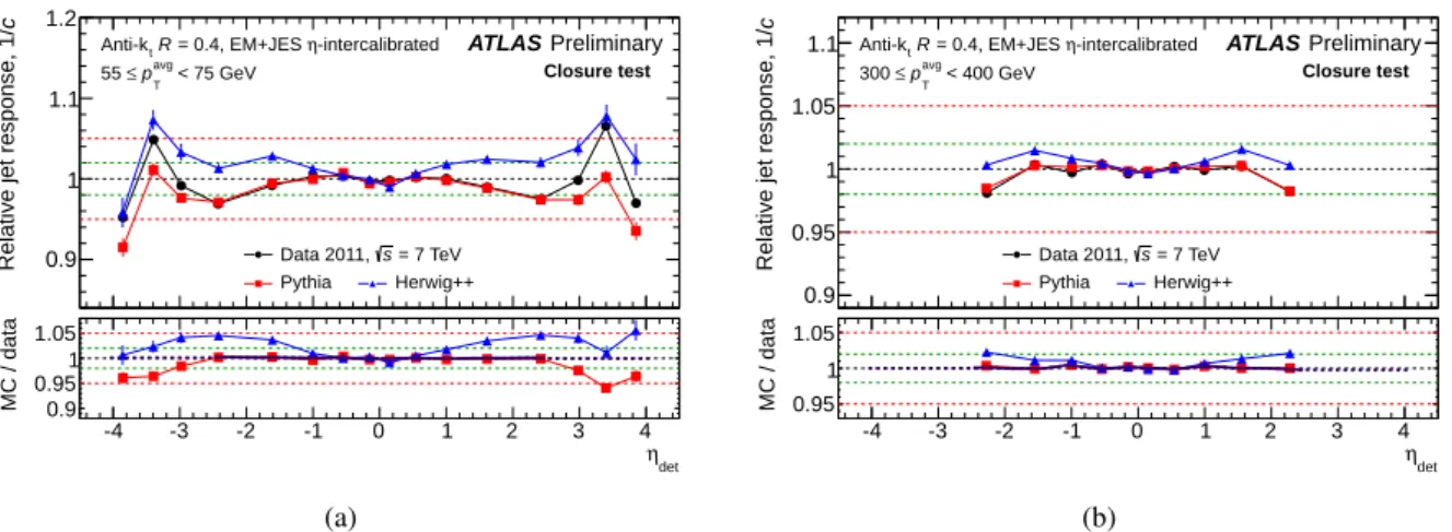
9 Validation using dijet, Z + jet and γ + jet data

To test the performance of the derived calibration, it was applied to all jets in the original dataset and the full analysis was repeated. The resulting intercalibration results are within 0.3% of unity across the full ( p

^avg_T

, η

_det

) phase space in which the calibration was derived, both for jets with R

=

0.4 and R

=

0.6, and for the EM

+

JES and LCW

+

JES calibrations. The measured relative response for two representative

p

^avg_T

-bins is shown in Figure

6.

Separate cross checks of forward jets were performed with Z

+jet and

γ

+jet data using the analyses

described in References [20] and [21]. The balance between a Z boson decaying to an electron-positron pair and a recoiling jet, and the balance between a photon and a jet, were used to study the jet response.

The results of these studies are presented in Figures

7

and

8. These measurements are consistent with the

results presented in this note within the assigned uncertainty. The Z

+jet study also includes predictions

from the A

lpgen

v2.13 generator [22] which uses H

erwig

v6.510 [10] for parton shower and fragmen- tation into particles. The Alpgen+Herwig response predictions generally agree with the expectations well within the modelling uncertainty of this analysis (see Section

8.1). The

γ

+jet results include com-

parisons with P

ythia

events, generated with the same tune and version as the P

ythia

dijet samples used in this analysis, and a sample produced with Herwig v6.510, using the ATLAS AUET2B MRST LO**

tune [12] and the MRST LO** PDF set.

(12)

1 1.1 1.2

-intercalibrated η

= 0.4, EM+JES

tR Anti-k

< 75 GeV

avg

pT

≤ 55

ATLAS Preliminary Closure test

ηdet

-4 -3 -2 -1 0 1 2 3 4

MC / data 0.9

0.95 1 1.05

(a)

0.9 0.95 1 1.05

1.1 Anti-k_tR = 0.4, EM+JES η-intercalibrated < 400 GeV

avg

pT

≤ 300

ATLAS Preliminary Closure test

ηdet

-4 -3 -2 -1 0 1 2 3 4

MC / data 0.95 1 1.05

(b)

Figure 6: Relative jet response, 1/c, as a function of the jet η

_det

for anti-k

t

jets with R

=

0.4 calibrated with the EM+JES scheme and in addition the derived η-intercalibration. Results are shown separately for 55

≤

p

^avg_T

< 75 GeV and 300

≤

p

^avg_T

< 400 GeV. For all points included in the original calibration (|η

_det|

< 2.8), the data are corrected to be consistent with the response of P

ythia

MC as intended. The resulting calibration derived from the already calibrated data is shown as a thick line and is consistent with unity.

jet| η

|

〉ref Tp / jet Tp 〈

0.4 0.5 0.6 0.7 0.8 0.9 1 1.1

< 35 GeV

ref

pT

≤ Z+jet, 25

ATLAS Preliminary Anti-k_tR = 0.4, EM+JES

Data Pythia Alpgen

η| jet |

0 0.5 1 1.5 2 2.5 3 3.5 4 4.5

MC / data

0.9 0.95 1 1.05

1.1 η intercalibration uncertainty in situ calibration

(a)

jet| η

|

〉ref Tp / jet Tp 〈

0.4 0.5 0.6 0.7 0.8 0.9 1 1.1

< 80 GeV

ref

pT

≤ Z+jet, 50

ATLAS Preliminary Anti-k_tR = 0.4, EM+JES

Data Pythia Alpgen

η| jet |

0 0.5 1 1.5 2 2.5 3 3.5 4 4.5

MC / data

0.9 0.95 1 1.05

1.1 η intercalibration uncertainty in situ calibration

(b)

Figure 7: Z

+

jet balance for anti-k

t

jets with R

=

0.4 calibrated with the EM

+

JES scheme with

25

≤

p

^ref_T

< 35 and 50

≤

p

^ref_T

< 80 GeV, where p

^ref_T

is the p

_T

of the reconstructed Z boson pro-

jected onto the axis of the balancing jet. As no in situ calibration is applied to these measurements, it is

expected that data and P

ythia

MC are shifted relative to each other by the absolute correction, presented

in Reference [

?

], multiplied by the relative, η

_det

-dependent correction, presented herein. The resulting in

situ JES calibration is shown as a solid line in the lower part of the figures. The modelling uncertainty is

shown as a filled band around the in situ correction.

(13)

jet| η

|

〉γ Tp / jet Tp 〈

0.4 0.5 0.6 0.7 0.8 0.9 1 1.1

< 110 GeV

γ

pT

≤ +jet, 85 γ

ATLAS Preliminary Anti-ktR = 0.4, EM+JES

Data Pythia Herwig++

η| jet |

0 0.5 1 1.5 2 2.5 3 3.5 4 4.5

MC / data

0.9 0.95 1 1.05 1.1

(a)

jet| η

|

〉γ Tp / jet Tp 〈

0.4 0.5 0.6 0.7 0.8 0.9 1 1.1

< 260 GeV

γ

pT

≤ +jet, 210 γ

ATLAS Preliminary Anti-ktR = 0.4, EM+JES

Data Pythia Herwig++

η| jet |

0 0.5 1 1.5 2 2.5 3 3.5 4 4.5

MC / data

0.9 0.95 1 1.05 1.1

(b)

Figure 8: γ

+jet balance for anti-kt

jets with R

=

0.4 calibrated with the EM+JES scheme with 85

≤

p

^γ_T

< 110 GeV and 210

≤

p

^γ_T

< 260 GeV. As no in situ calibration is applied to these measurements, it is expected that data and Pythia MC are shifted relative to each other by the absolute correction, presented in Reference [?], multiplied by the relative, η

_det

-dependent correction, presented herein. This total, in situ JES calibration is shown as a solid line in the lower part of the figures. The dijet modelling uncertainty is shown as a filled band around the in situ correction.

10 Summary

The pseudorapidity dependence of the jet response was studied using dijet pseudorapidity intercalibra- tion. A residual, p

_T

and η dependent jet calibration was derived for jets in data with

|η_det|

< 2.4 to correct for e

ff

ects not captured by the default Monte Carlo derived calibration. The corrected calibration was measured to approximately

+

1% at

|η_det| =

1.0 and falling to

−3% to −1% for|η_det| =

2.4 and beyond. The uncertainty on the calibration increases as a function of

|η_det|

and decreases with p

_T

. For a p

_T =

25 GeV jet, the uncertainty is about 1% at

|η_det| =

1.0, 3% at

|η_det| =

2.0 and about 5% for

|η_det|

> 3.0. The uncertainty is below 1% for p

_T=

500 GeV jets with

|η_det|

< 2.

References

[1] ATLAS Collaboration, Jet energy measurement with the ATLAS detector in proton-proton collisions at

√

s

=

7 TeV, Submitted to EPJ (2011) ,

arXiv:1112.6426 [hep-ex].

[2] ATLAS Collaboration, Single hadron response measurement and calorimeter jet energy scale uncertainty in the ATLAS detector at the LHC, submitted to EPJ (2012) ,

arXiv:1203.1302 [hep-ex].

[3] ATLAS Collaboration, In-situ pseudo-rapidity inter-calibration to evaluate jet energy scale uncertainty and calorimeter performance in the forward region,

ATLAS-CONF-2010-055, June,

2010. ATLAS Collaboration, In situ pseudorapidity intercalibration for evaluation of jet energy scale uncertainty using dijet events in proton-proton collisions at

√

s

=

7 TeV,

ATLAS-CONF-2011-014, February, 2011.

[4] ATLAS Collaboration, Expected performance of the ATLAS experiment - detector, trigger and

physics, , September, 2009.

arXiv:0901.0512 [hep-ex]. CERN-OPEN-2008-020.

(14)

[5] T. Sjostrand, S. Mrenna, and P. Z. Skands, PYTHIA 6.4 physics and manual, JHEP

0605

(2006) 026,

arXiv:0603175 [hep-ph].

[6] R. Corke and T. Sjostrand, Improved Parton Showers at Large Transverse Momenta, Eur. Phys. J.

C 69

(2010) 1–18,

arXiv:1003.2384 [hep-ph].

[7] A. Sherstnev and R. S. Thorne, Parton distributions for LO generators, Eur. Phys. J.

C 55

(2008) 553–575,

[8] M. Bahr et al., Herwig

++

physics and manual, Eur. Phys. J.

C 58

(2008) 639–707,

[9] G. Marchesini et al., Monte Carlo simulation of general hard processes with coherent QCD radiation, Nucl. Phys.

B 310

(1988) 461. G. Marchesini et al., A Monte Carlo event generator for simulating hadron emission reactions with interfering gluons, Comput. Phys. Commun.

67

(1991) 465–508.

[10] G. Corcella et al., HERWIG 6.5 release note,

[11] M. Bahr, S. Gieseke, and M. H. Seymour, Simulation of multiple partonic interactions in Herwig

++, JHEP07

(2008) 076,

[12] ATLAS Collaboration, ATLAS tunes for Pythia6 and Pythia8 for MC11,

ATLAS-PHYS-PUB-2011-009, July, 2011.

[13] T. Sjostrand, S. Mrenna, and P. Z. Skands, A Brief Introduction to PYTHIA 8.1,

Comput. Phys.

Commun.178(2008) 852–867,arXiv:0710.3820 [hep-ph].

[14] M. Cacciari, G. P. Salam, and G. Soyez, The anti-k

_t

jet clustering algorithm, JHEP

04

(2008) 063,

[15] M. Cacciari and G. P. Salam, Dispelling the N

³

myth for the k

t

jet-finder, Phys. Lett. B

641

(2006) 57–61. M. Cacciari, G. P. Salam, and G. Soyez.

http://fastjet.fr/.

[16] C. Cojocaru et al., Hadronic calibration of the ATLAS liquid argon end-cap calorimeter in the pseudorapidity region 1.6 <

|η|

< 1.8 in beam tests, Nucl. Instrum. Meth.

A 531

(2004) 481–514.

[17] W. Lampl et al., Calorimeter clustering algorithms: description and performance,

ATL-LARG-PUB-2008-002, April, 2008.

[18] V. Lendermann et al., Combining Triggers in HEP Data Analysis,

Nucl. Instrum. Meth.A604 (2009) 707–718,arXiv:0901.4118 [hep-ex].

[19] ATLAS Collaboration, Pile-up corrections for jets from proton-proton collisions at

√

s

=

7 TeV in ATLAS in 2011,

ATLAS-CONF-2012-064, June, 2012.

[20] ATLAS Collaboration, Probing the measurement of jet energies with the ATLAS detector using Z+jet events from proton-proton collisions at

√

s

=

7 TeV,

ATLAS-CONF-2012-053, May, 2012.

[21] ATLAS Collaboration, XXX photon-jet events in proton-proton collisions at

√

s

=

7 TeV ,

ATLAS-CONF-2012-XXX, June, 2012.

[22] M. L. Mangano, M. Moretti, F. Piccinini, R. Pittau, and A. D. Polosa, ALPGEN, a generator for

hard multiparton processes in hadronic collisions, JHEP

07