Study of Jet Shapes in Inclusive Jet Production in pp Collisions at √s = 7 TeV using the ATLAS Detector

arXiv:1101.0070v1 [hep-ex] 30 Dec 2010

the ATLAS Detector

(The ATLAS Collaboration) (Dated: January 4, 2011)

Jet shapes have been measured in inclusive jet production in proton-proton collisions at √

s =

7 TeV using 3 pb

of data recorded by the ATLAS experiment at the LHC. Jets are reconstructed using the anti-k

algorithm with transverse momentum 30 GeV < p

< 600 GeV and rapidity in the region | y | < 2.8. The data are corrected for detector effects and compared to several leading- order QCD matrix elements plus parton shower Monte Carlo predictions, including different sets of parameters tuned to model fragmentation processes and underlying event contributions in the final state. The measured jets become narrower with increasing jet transverse momentum and the jet shapes present a moderate jet rapidity dependence. Within QCD, the data test a variety of perturbative and non-perturbative effects. In particular, the data show sensitivity to the details of the parton shower, fragmentation, and underlying event models in the Monte Carlo generators. For an appropriate choice of the parameters used in these models, the data are well described.

PACS numbers: 13.85.Ni, 13.85.Qk, 14.65.Ha, 87.18.Sn

I. INTRODUCTION

The study of the jet shapes [1] in proton-proton collisions provides information about the details of the parton- to-jet fragmentation process, leading to collimated flows of particles in the final state. The internal structure of sufficiently energetic jets is mainly dictated by the emission of multiple gluons from the primary parton, calculable in perturbative QCD (pQCD) [2]. The shape of the jet depends on the type of partons (quark or gluon) that give rise to jets in the final state [3], and is also sensitive to non-perturbative fragmentation effects and underlying event (UE) contributions from the interaction between proton remnants. A proper modeling of the soft contributions is crucial for the understanding of jet production in hadron-hadron collisions and for the comparison of the jet cross section measurements with pQCD theoretical predictions [4, 5]. In addition, jet shape related observables have been recently proposed [6] to search for new physics in event topologies with highly boosted particles in the final state decaying into multiple jets of particles.

Jet shape measurements have previously been performed in p¯ p [7], e

p [8], and e ⁺ e

[9] collisions. In this paper, measurements of differential and integrated jet shapes in proton-proton collisions at √

s = 7 TeV are presented for the first time. The study uses data collected by the ATLAS experiment corresponding to 3 pb

¹ of total integrated luminosity. The measurements are corrected for detector effects and compared to several Monte Carlo (MC) predictions based on pQCD leading-order (LO) matrix elements plus parton showers, and including different phenomenological models to describe fragmentation processes and UE contributions.

The paper is organised as follows. The detector is described in the next section. Section 3 discusses the simulations used in the measurements, while Section 4 and Section 5 provide details on jet reconstruction and event selection, respectively. Jet shape observables are defined in Section 6. The procedure used to correct the measurements for detector effects is explained in Section 7, and the study of systematic uncertainties is discussed in Section 8. The jet shape measurements are presented in Section 9. Finally, Section 10 is devoted to summary and conclusions.

II. EXPERIMENTAL SETUP

The ATLAS detector [10] covers nearly the entire solid angle around the collision point with layers of tracking detectors, calorimeters, and muon chambers. For the measurements presented in this paper, the tracking system and calorimeters are of particular importance.

The ATLAS inner detector has full coverage in φ [11] and covers the pseudorapidity range | η | < 2.5. It consists of a silicon pixel detector, a silicon microstrip detector and a transition radiation tracker, all immersed in a 2 Tesla magnetic field. High granularity liquid-argon (LAr) electromagnetic sampling calorimeters cover the pseudorapidity range | η | < 3.2. The hadronic calorimetry in the range | η | < 1.7 is provided by a scintillator-tile calorimeter, which is separated into a large barrel and two smaller extended barrel cylinders, one on either side of the central barrel. In the end-caps ( | η | > 1.5), LAr hadronic calorimeters match the outer | η | limits of the end-cap electromagnetic calorimeters.

The LAr forward calorimeters provide both electromagnetic and hadronic energy measurements, and they extend the

coverage to | η | < 4.9.

The trigger system uses three consecutive trigger levels to select events. The Level-1 (L1) trigger is based on custom-built hardware to process the incoming data with a fixed latency of 2.5 µs. This is the only trigger level used in this analysis. The events studied here are selected either by the system of minimum-bias trigger scintillators (MBTS) or by the calorimeter trigger. The MBTS detector [12] consists of 32 scintillator counters of thickness 2 cm organized in two disks. The disks are installed on the inner face of the end-cap calorimeter cryostats at z = ± 356 cm, such that the disk surface is perpendicular to the beam direction. This leads to a coverage of 2.09 < | η | < 3.84. The jet trigger is based on the selection of jets according to their transverse energy, E

. The L1 jet reconstruction uses the so called jet elements, which are made of electromagnetic and hadronic cells grouped together with a granularity of ∆φ × ∆η = 0.2 × 0.2 for | η | < 3.2. The jet finding is based on a sliding window algorithm with steps of one jet element, and the jet E

is computed in a window of configurable size around the jet.

III. MONTE CARLO SIMULATION

Monte Carlo simulated samples are used to determine and correct for detector effects, and to estimate part of the systematic uncertainties on the measured jet shapes. Samples of inclusive jet events in proton-proton collisions at

√ s = 7 TeV are produced using both PYTHIA 6.4.21 [13] and HERWIG++ 2.4.2 [14] event generators. These MC programs implement LO pQCD matrix elements for 2 → 2 processes plus parton shower in the leading logarithmic approximation, and the string [15] and cluster [16] models for fragmentation into hadrons, respectively. In the case of PYTHIA, different MC samples with slightly different parton shower and UE modeling in the final state are considered. The samples are generated using three tuned sets of parameters denoted as ATLAS-MC09 [17], DW [18], and Perugia2010 [19]. In addition, a special PYTHIA-Perugia2010 sample without UE contributions is generated.

Finally, inclusive jet samples are also produced using the ALPGEN 2.13 [20] event generator interfaced with HERWIG 6.5 [21] and JIMMY 3.41 [22] to model the UE contributions. HERWIG++ and PYTHIA-MC09 samples are generated with MRST2007LO

[23] parton density functions (PDFs) inside the proton, PYTHIA-Perugia2010 and PYTHIA-DW with CTEQ5L [24] PDFs, and ALPGEN with CTEQ61L [25] PDFs.

The MC generated samples are passed through a full simulation [26] of the ATLAS detector and trigger, based on GEANT4 [27]. The Quark Gluon String Precompound (QGSP) model [28] is used for the fragmentation of the nucleus, and the Bertini cascade (BERT) model [29] for the description of the interactions of the hadrons in the medium of the nucleus. Test-beam measurements for single pions have shown that these simulation settings best describe the response and resolution in the barrel [30] and end-cap [31] calorimeters. The simulated events are then reconstructed and analyzed with the same analysis chain as for the data, and the same trigger and event selection criteria.

IV. JET RECONSTRUCTION

Jets are defined using the anti-k

jet algorithm [32] with distance parameter (in y − φ space) R = 0.6, and the energy depositions in calorimeter clusters as input in both data and MC events. Topological clusters [5] are built around seed calorimeter cells with | E cell | > 4σ, where σ is defined as the RMS of the cell energy noise distribution, to which all directly neighboring cells are added. Further neighbors of neighbors are iteratively added for all cells with signals above a secondary threshold | E cell | > 2σ, and the clusters are set massless. In addition, in the simulated events jets are also defined at the particle level [33] using as input all the final state particles from the MC generation.

The anti-k

algorithm constructs, for each input object (either energy cluster or particle) i, the quantities d

and d

as follows:

d

= min(k

² , k

² ) (∆R) ²

R ² , (1)

d

= k

, (2)

where

(∆R) ²

= (y

− y

) ² + (φ

− φ

) ² , (3)

k

is the transverse momentum of object i with respect to the beam direction, φ

its azimuthal angle, and y

its

rapidity. A list containing all the d

and d

values is compiled. If the smallest entry is a d

, objects i and j are

combined (their four-vectors are added) and the list is updated. If the smallest entry is a d

, this object is considered

a complete “jet” and is removed from the list. As defined above, d

is a distance measure between two objects, and

Trigger Information

p

(GeV) trigger configurations integrated luminosity (nb

)

30 - 60 MBTS 0.7

60 - 80 L1 5/MBTS 17

80 - 110 L1 10/L1 5/MBTS 96

110 - 160 L1 15/L1 10/L1 5/MBTS 545

160 - 210 L1 30/L1 15/L1 10/L1 5/MBTS 1878 210 - 600 L1 55/L1 30/L1 15/L1 10/L1 5/MBTS 2993

TABLE I: For the various jet p

ranges, the trigger configurations used to collect the data and the corresponding total integrated luminosity. MBTS denotes the use of the minimum-bias trigger scintillators, while L1 5, L1 10, L1 15, L1 30, and L1 55 correspond to L1 calorimeter triggers with 5, 10, 15, 30, and 55 GeV thresholds, respectively.

d

is a similar distance between the object and the beam. Thus the variable R is a resolution parameter which sets the relative distance at which jets are resolved from each other as compared to the beam. The anti-k

algorithm is theoretically well-motivated [32] and produces geometrically well-defined (“cone-like”) jets.

According to MC simulation, the measured jet angular variables, y and φ, are reconstructed with a resolution of better than 0.05 units, which improves as the jet transverse momentum, p

, increases. The measured jet p

is corrected to the particle level scale [5] using an average correction, computed as a function of jet transverse momentum and pseudorapidity, and extracted from MC simulation.

V. EVENT SELECTION The data were collected during the first LHC run at √

s = 7 TeV with the ATLAS tracking detectors, calorimeters and magnets operating at nominal conditions. Events are selected online using different L1 trigger configurations in such a way that, in the kinematic range for the jets considered in this study (see below), the trigger selection is fully efficient and does not introduce any significant bias in the measured jet shapes. Table 1 presents the trigger configurations employed in each p

region and the corresponding integrated luminosity. The unprescaled trigger thresholds were increased with time to keep pace with the LHC instantaneous luminosity evolution. For jet p

smaller than 60 GeV, the data are selected using the signals from the MBTS detectors on either side of the interaction point. Only events in which the MBTS recorded one or more counters above threshold on at least one side are retained. For larger p

, the events are selected using either MBTS or L1 calorimeter based triggers (see Section 2) with a minimum transverse energy threshold at the electromagnetic scale [34] that varies between 5 GeV (L1 5) and 55 GeV (L1 55), depending on when the data were collected and the p

range considered (see Table 1).

The events are required to have one and only one reconstructed primary vertex with a z-position within 10 cm of the origin of the coordinate system, which suppresses pile-up contributions from multiple proton-proton interactions in the same bunch crossing, beam-related backgrounds and cosmic rays. In this analysis, events are required to have at least one jet with corrected transverse momentum p

> 30 GeV and rapidity | y | < 2.8. This corresponds approximately to the kinematic region, in the absolute four momentum transfer squared Q ² - Bjorken-x plane, of 10 ³ GeV ² < Q ² < 4 × 10 ⁵ GeV ² and 6 × 10

< x < 2 × 10

. Additional quality criteria are applied to ensure that jets are not produced by noisy calorimeter cells, and to avoid problematic detector regions.

VI. JET SHAPE DEFINITION

The internal structure of the jet is studied in terms of the differential and integrated jet shapes, as reconstructed using the uncorrected energy clusters in the calorimeter associated with the jet. The differential jet shape ρ(r) as a function of the distance r = p

∆y ² + ∆φ ² to the jet axis is defined as the average fraction of the jet p

that lies inside an annulus of inner radius r − ∆r/2 and outer radius r + ∆r/2 around the jet axis:

ρ(r) = 1

∆r 1 N ^jet

X

jets

p

(r − ∆r/2, r + ∆r/2)

p

(0, R) , ∆r/2 ≤ r ≤ R − ∆r/2, (4)

where p

(r 1 , r 2 ) denotes the summed p

of the clusters in the annulus between radius r 1 and r 2 , N ^jet is the number of

jets, and R = 0.6 and ∆r = 0.1 are used. The points from the differential jet shape at different r values are correlated since, by definition, P

0 ρ(r) ∆r = 1. Alternatively, the integrated jet shape Ψ(r) is defined as the average fraction of the jet p

that lies inside a cone of radius r concentric with the jet cone:

Ψ(r) = 1 N ^jet

X

jets

p

(0, r)

p

(0, R) , 0 ≤ r ≤ R, (5)

where, by definition, Ψ(r = R) = 1, and the points at different r values are correlated. The same definitions apply to simulated calorimeter clusters and final-state particles in the MC generated events to define differential and integrated jet shapes at the calorimeter and particle levels, respectively. The jet shape measurements are performed in different regions of jet p

and | y | , and a minimum of 100 jets in data are required in each region to limit the statistical fluctuations on the measured values.

VII. CORRECTION FOR DETECTOR EFFECTS

The measured differential and integrated jet shapes, as determined by using calorimeter topological clusters, are corrected for detector effects back to the particle level. This is done using MC simulated events and a bin-by-bin correction procedure that also accounts for the efficiency of the selection criteria and of the jet reconstruction in the calorimeter. PYTHIA-Perugia2010 provides a reasonable description of the measured jet shapes in all regions of jet p

and | y | , and is therefore used to compute the correction factors. Here, the method is described in detail for the differential case. A similar procedure is employed to correct independently the integrated measurements. The correction factors U (r, p

, | y | ) are computed separately in each jet p

and | y | region. They are defined as the ratio between the jet shapes at the particle level ρ(r)

, obtained using particle-level jets in the kinematic range under consideration, and the reconstructed jet shapes at the calorimeter level ρ(r)

, after the selection criteria are applied and using calorimeter-level jets in the given p

and | y | range. The correction factors U (r, p

, | y | ) = ρ(r)

/ρ(r)

present a moderate p

and | y | dependence and vary between 0.95 and 1.1 as r increases. For the integrated jet shapes, the correction factors differ from unity by less than 5%. The corrected jet shape measurements in each p

and | y | region are computed by multiplying bin-by-bin the measured uncorrected jet shapes in data by the corresponding correction factors.

VIII. SYSTEMATIC UNCERTAINTIES

A detailed study of systematic uncertainties on the measured differential and integrated jet shapes has been per- formed. The impact on the differential measurements is described here in detail.

• The absolute energy scale of the individual clusters belonging to the jet is varied in the data according to studies using isolated tracks [5], which parametrize the uncertainty on the calorimeter cluster energy as a function of p

and η of the cluster. This introduces a systematic uncertainty on the measured differential jet shapes that varies between 3% to 15% as r increases and constitutes the dominant systematic uncertainty in this analysis.

• The systematic uncertainty on the measured jet shapes arising from the details of the model used to sim- ulate calorimeter showers in the MC events is studied. A different simulated sample is considered, where the FRITIOF [35] plus BERT showering model is employed instead of the QGSP plus BERT model.

FRITOF+BERT provides the second best description of the test-beam results [30] after QGSP+BERT. This introduces an uncertainty on the measured differential jet shapes that varies between 1% to 4%, and is approx- imately independent of p

and | y | .

• The measured jet p

is varied by 2% to 8%, depending on p

and | y | , to account for the remaining uncertainty on the absolute jet energy scale [5], after removing contributions already accounted for and related to the energy of the single clusters and the calorimeter shower modeling, as discussed above. This introduces an uncertainty of about 3% to 5% in the measured differential jet shapes.

• The 14% uncertainty on the jet energy resolution [5] translates into a smaller than 2% effect on the measured

differential jet shapes.

• The correction factors are recomputed using HERWIG++, which implements different parton shower, frag- mentation and UE models than PYTHIA, and compared to PYTHIA-Perugia2010. In addition, the correction factors are also computed using ALPGEN and PYTHIA-DW for p

< 110 GeV, where these MC samples pro- vide a reasonable description of the uncorrected shapes in the data. The results from HERWIG++ encompass the variations obtained using all the above generators and are conservatively adopted in all p

and | y | ranges to compute systematic uncertainties on the differential jet shapes. These uncertainties increase between 2% and 10% with increasing r.

• An additional 1% uncertainty on the differential measurements is included to account for deviations from unity (non-closure) in the bin-by-bin correction procedure when applied to a statistically independent MC sample.

• No significant dependence on instantaneous luminosity is observed in the measured jet shapes, indicating that residual pile-up contributions are negligible after selecting events with only one reconstructed primary vertex.

• It was verified that the presence of small dead calorimeter regions in the data does not affect the measured jet shapes.

The different systematic uncertainties are added in quadrature to the statistical uncertainty to obtain the final result.

The total uncertainty for differential jet shapes decreases with increasing p

and varies typically between 3% and 10% (10% and 20%) at r = 0.05 (r = 0.55). The total uncertainty is dominated by the systematic uncertainty, except at very large p

where the measurements are still statistically limited. In the case of the integrated measurements, the total systematic uncertainty varies between 10% and 2% (4% and 1%) at r = 0.1 (r = 0.3) as p

increases, and vanishes as r approaches the edge of the jet cone.

Finally, the jet shape analysis is also performed using either tracks from the inner detector inside the jet cone, as reconstructed using topological clusters; or calorimeter towers of fixed size 0.1 × 0.1 (y − φ space) instead of topological clusters as input to the jet reconstruction algorithm. For the former, the measurements are limited to jets with | y | < 1.9, as dictated by the tracking coverage and the chosen size of the jet. After the data are corrected back to particle level, the results from these alternative analyses are consistent with the nominal results, with maximum deviations in the differential measurements of about 2% (5%) at r=0.05 (r=0.55), well within the quoted systematic uncertainties.

IX. RESULTS

The measurements presented in this article refer to differential and integrated jet shapes, ρ(r) and Ψ(r), corrected at the particle level and obtained for anti-k

jets with distance parameter R = 0.6 in the region | y | < 2.8 and 30 GeV < p

< 600 GeV. The measurements are presented in separate bins of p

and | y | . Tabulated values of the results are available in the Appendix and in Ref. [36].

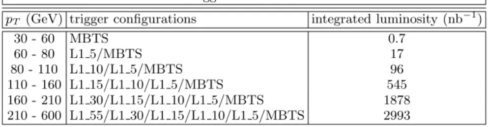
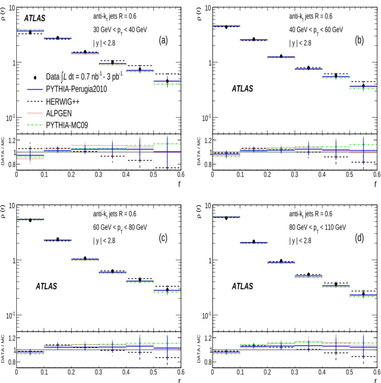
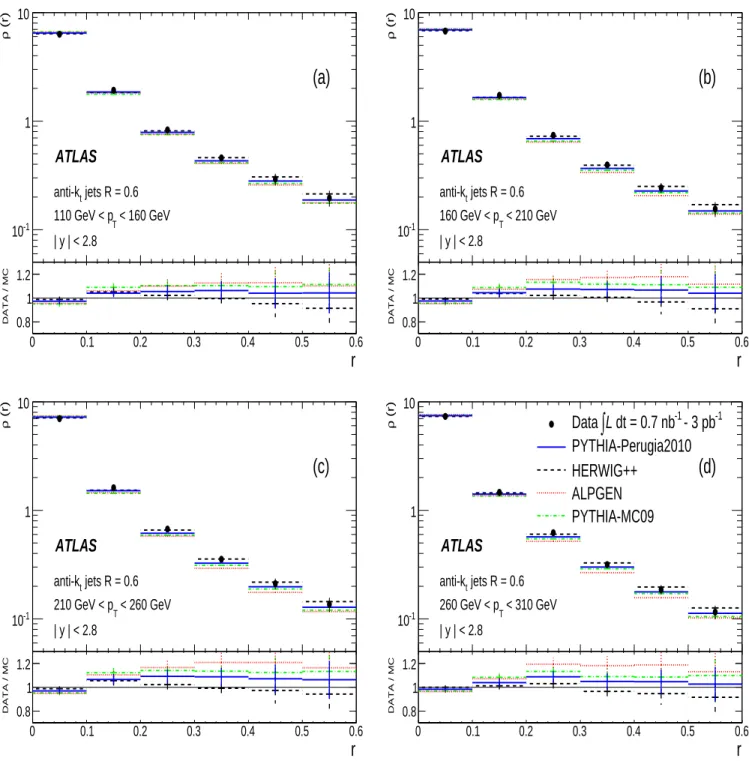
Figures 1 to 3 show the measured differential jet shapes as a function of r in different p

ranges. The dominant peak at small r indicates that the majority of the jet momentum is concentrated close to the jet axis. At low p

, more than 80% of the transverse momentum is contained within a cone of radius r = 0.3 around the jet direction.

This fraction increases up to 95% at very high p

, showing that jets become narrower as p

increases. This is also observed in Fig. 4, where the measured 1 − Ψ(0.3), the fraction of the jet transverse momentum outside a fixed radius r = 0.3, decreases as a function of p

.

The data are compared to predictions from HERWIG++, ALPGEN, PYTHIA-Perugia2010, and PYTHIA-MC09 in Fig. 1 to Fig. 4(a); and to predictions from PYTHIA-DW and PYTHIA-Perugia2010 with and without UE con- tributions in Fig. 4(b). The jet shapes predicted by PYTHIA-Perugia2010 provide a reasonable description of the data, while HERWIG++ predicts broader jets than the data at low and very high p

. The PYTHIA-DW predictions are in between PYTHIA-Perugia2010 and HERWIG++ at low p

and produce jets which are slightly narrower at high p

. ALPGEN is similar to PYTHIA-Perugia2010 at low p

, but produces jets significantly narrower than the data at high p

. PYTHIA-MC09 tends to produce narrower jets than the data in the whole kinematic range under study. The latter may be attributed to an inadequate modeling of the soft gluon radiation and UE contributions in PYTHIA-MC09 samples, in agreement with previous observations of the particle flow activity in the final state [12].

Finally, Fig. 4(b) shows that PYTHIA-Perugia2010 without UE contributions predicts jets much narrower than the data at low p

. This confirms the sensitivity of jet shape observables in the region p

< 160 GeV to a proper description of the UE activity in the final state.

The dependence on | y | is shown in Fig. 5, where the measured jet shapes are presented separately in five different jet

rapidity regions and different p

bins, for jets with p

< 400 GeV. At high p

, the measured 1 − Ψ(0.3) shape presents

a mild | y | dependence, indicating that the jets become slightly narrower in the forward regions. This tendency is

observed also in the various MC samples. Similarly, Figs. 6 and 7 present the measured 1 − Ψ(0.3) as a function of p

in the different | y | regions compared to PYTHIA-Perugia2010 predictions. The result of χ ² tests to the data in Fig. 7 with respect to the predictions from the different MC generators are reported in Table 7, for each of the five rapidity regions. Here the different sources of systematic uncertainty are considered independent and fully correlated across p

bins (see Appendix). As already discussed, PYTHIA-Perugia2010 provides the best overall description of the data, while PYTHIA-Perugia2010 without UE contributions and ALPGEN show the largest discrepancies.

Finally, and only for illustration, the typical shapes of quark- and gluon-initiated jets, as determined using events generated with PYTHIA-Perugia2010, are also shown in Figs. 6 and 7. For this purpose, MC events are selected with at least two particle-level jets with p

> 30 GeV and | y | < 2.8 in the final state. The two leading jets in this dijet sample are classified as quark-initiated or gluon-initiated jets by matching (in y − φ space) their direction with one of the outgoing partons from the QCD 2 → 2 hard process. At low p

the measured jet shapes are similar to those from gluon-initiated jets, as expected from the dominance of hard processes with gluons in the final state. At high p

, where the impact of the UE contributions becomes smaller (see Fig. 4(b)), the observed trend with p

in the data is mainly attributed to a changing quark- and gluon-jet mixture in the final state, convoluted with perturbative QCD effects related to the running of the strong coupling.

X. SUMMARY AND CONCLUSIONS

In summary, jet shapes have been measured in inclusive jet production in proton-proton collisions at √

s = 7 TeV using 3 pb

¹ of data recorded by the ATLAS experiment at the LHC. Jets are reconstructed using the anti-k

algorithm with distance parameter R = 0.6 in the kinematic region 30 GeV < p

< 600 GeV and | y | < 2.8. The data are corrected for detector effects and compared to different leading-order matrix elements plus parton shower MC predictions. The measured jets become narrower as the jet transverse momentum and rapidity increase, although with a rather mild rapidity dependence. The data are reasonably well described by PYTHIA-Perugia2010. HERWIG++

predicts jets slightly broader than the data, whereas ALPGEN interfaced with HERWIG and JIMMY, PYTHIA-DW, and PYTHIA-MC09 all predict jets narrower than the data. Within QCD, the data show sensitivity to a variety of perturbative and non-perturbative effects. The results reported in this paper indicate the potential of jet shape measurements at the LHC to constrain the current phenomenological models for soft gluon radiation, UE activity, and non-perturbative fragmentation processes in the final state.

XI. ACKNOWLEDGEMENTS

We wish to thank CERN for the efficient commissioning and operation of the LHC during this initial high-energy data-taking period as well as the support staff from our institutions without whom ATLAS could not be operated efficiently.

We acknowledge the support of ANPCyT, Argentina; YerPhI, Armenia; ARC, Australia; BMWF, Austria; ANAS, Azerbaijan; SSTC, Belarus; CNPq and FAPESP, Brazil; NSERC, NRC and CFI, Canada; CERN; CONICYT, Chile;

CAS, MOST and NSFC, China; COLCIENCIAS, Colombia; MSMT CR, MPO CR and VSC CR, Czech Republic;

DNRF, DNSRC and Lundbeck Foundation, Denmark; ARTEMIS, European Union; IN2P3-CNRS, CEA-DSM/IRFU, France; GNAS, Georgia; BMBF, DFG, HGF, MPG and AvH Foundation, Germany; GSRT, Greece; ISF, MINERVA, GIF, DIP and Benoziyo Center, Israel; INFN, Italy; MEXT and JSPS, Japan; CNRST, Morocco; FOM and NWO, Netherlands; RCN, Norway; MNiSW, Poland; GRICES and FCT, Portugal; MERYS (MECTS), Romania; MES of Russia and ROSATOM, Russian Federation; JINR; MSTD, Serbia; MSSR, Slovakia; ARRS and MVZT, Slovenia;

DST/NRF, South Africa; MICINN, Spain; SRC and Wallenberg Foundation, Sweden; SER, SNSF and Cantons of Bern and Geneva, Switzerland; NSC, Taiwan; TAEK, Turkey; STFC, the Royal Society and Leverhulme Trust, United Kingdom; DOE and NSF, United States of America.

The crucial computing support from all WLCG partners is acknowledged gratefully, in particular from CERN and the ATLAS Tier-1 facilities at TRIUMF (Canada), NDGF (Denmark, Norway, Sweden), CC-IN2P3 (France), KIT/GridKA (Germany), INFN-CNAF (Italy), NL-T1 (Netherlands), PIC (Spain), ASGC (Taiwan), RAL (UK) and BNL (USA) and in the Tier-2 facilities worldwide.

[1] S. D. Ellis, Z. Kunszt and D. E. Soper, Phys. Rev. Lett. 69 3615 (1992).

[2] D. J. Gross and F. Wilczek, Phys. Rev. D 8 3633 (1973).

[3] Inclusive jet shape studies have a very limited sensitivity to the presence of a small contribution from heavy-flavor quarks in the final state.

[4] The CDF Collaboration, A. Abulencia et al. , Phys. Rev. D 75 092006 (2007).

The D0 Collaboration, V. M. Abazov et al. , Phys. Rev. Lett. 101 062001 (2008).

The CDF Collaboration, T. Aaltonen et al. , Phys. Rev. D 78 052006 (2008).

[5] The ATLAS Collaboration, G. Aad et al. , CERN-PH-EP-2010-034; arXiv:1009.5908 (2010); accepted for publication in Eur. Phys. J. C, and references therein.

[6] J. M. Butterworth, A. R. Davison, M. Rubin and G. P. Salam, Phys. Rev. Lett. 100 242001 (2008).

D. Kaplan et al. , Phys. Rev. Lett. 101 142001 (2008).

G. Salam, Eur. Phys. J. C 67 637 (2010).

[7] The CDF Collaboration, D. Acosta et al. , Phys. Rev. D 71 112002 (2005).

The CDF Collaboration, F. Abe et al. , Phys. Rev. Lett. 70 713 (1993).

The D0 Collaboration, S. Abachi et al. , Phys. Lett. B 357 500 (1995).

[8] The ZEUS Collaboration, S. Chekanov et al. , Nucl. Phys. B 700 3 (2004).

The ZEUS Collaboration, J.Breitweg et al. , Eur. Phys. J. C 8 3 367 (1999).

The H1 Collaboration, C. Adloff et al. , Nucl. Phys. B 545 3 (1999).

The ZEUS Collaboration, J.Breitweg et al. , Eur. Phys. J. C 2 1 61 (1998).

[9] The OPAL Collaboration, R. Akers et al. , Z. Phys. C 63 197 (1994).

The OPAL Collaboration, K. Ackerstaff et al. , Eur. Phys. J. C 1 479 (1998).

[10] The ATLAS Collaboration, G. Aad et al. , JINST 3 S08003 (2008).

[11] The ATLAS reference system is a Cartesian right-handed coordinate system, with the nominal collision point at the origin.

The anti-clockwise beam direction defines the positive z-axis, while the positive x-axis is defined as pointing from the collision point to the centre of the LHC ring and the positive y-axis points upwards. The azimuthal angle φ is measured around the beam axis, and the polar angle θ is measured with respect to the z-axis. The pseudorapidity is defined as η = − ln(tan(θ/2)). The rapidity is defined as y = 0.5 × ln[(E + p

)/(E − p

)], where E denotes the energy and p

is the component of the momentum along the beam direction.

[12] The ATLAS Collaboration, G. Aad et al. , Phys. Lett. B 688 21 (2010).

[13] T. Sj¨ ostrand et al. , JHEP 05 026 (2006).

[14] M. Bahr et al. , HERWIG++ Physics and Manual, Eur. Phys. J. C 58 639 (2008).

[15] B. Andersson et al. , Phys. Rep. 97 31 (1983).

[16] B.R. Webber, Nucl. Phys. B 238 492 (1984).

[17] ATLAS Collaboration, ATLAS MC tunes for MC09, ATL-PHYS-PUB-2010-002 (2010).

[18] The CDF Collaboration, T. Aaltonen et al. , Phys. Rev. D 82 034001 (2010).

[19] P. Z. Skands, CERN-PH-TH-2010-113, arXiv:hep-ph/1005.3457 (2010).

[20] M.L. Mangano et al. , JHEP 01 0307 (2003).

[21] G. Corcella et al. , JHEP 0101 010 (2001).

[22] J. Butterworth, J. Forshaw and M.Seymour, Z. Phys. C 72 637 (1996).

[23] A. D. Martin, W. J. Stirling, R. S. Thorne and G. Watt, Eur. Phys. J. C 63 189 (2009).

A. Sherstnev and R. S. Thorne, Eur. Phys. J. C 55 553 (2008).

[24] J. Pumplin et al. , JHEP 0207 012 (2002).

[25] D. Stump et al. , JHEP 0310 046 (2003).

[26] The ATLAS Collaboration, G. Aad et al. , Eur. Phys. J. C 70 823 (2010).

[27] S. Agostinelli et al. , Nucl. Instrum. and Meth. A506 250 (2003).

[28] G. Folger and J.P. Wellisch, arXiv:nucl-th/0306007 (2003).

[29] H. Bertini, Phys. Rev. 188 1711 (1969).

[30] E. Abat et al. , Tech. Rep. ATL-CAL-PUB-2010-001, CERN, Geneva, (2010).

P. Adragna et al. , CERN-PH-EP-2009-019; ATL-TILECAL-PUB-2009-009 (2009).

E. Abat et al. , Nucl. Instrum. and Meth. A607 372 (2009).

E. Abat et al. , Nucl. Instrum. and Meth. A615 158 (2010).

E. Abat et al. , Nucl. Instrum. and Meth. A621 134 (2010).

[31] J. Pinfold et al. , Nucl. Instrum. Meth. A593 324 (2008).

D. M. Gingrich et al., J. Inst. 2 no. 05 P05005 (2007).

[32] M. Cacciari, G. P. Salam and G. Soyez, JHEP 0804 063 (2008).

[33] The final state in the MC generators is defined using all particles (including muons and neutrinos) with lifetime above 10

s.

[34] The electromagnetic scale is the appropriate scale for the reconstruction of the energy deposited by electrons or photons in the calorimeter.

[35] B. Andersson, G. Gustafson and B. Nilsson-Almqvist, Nucl. Phys. B 281 289 (1987).

[36] A complete set of tables for differential and integrated measurements as a function of p

and | y | are available at the

Durham HepData repository (http://hepdata.cedar.ac.uk).

0 0.1 0.2 0.3 0.4 0.5 0.6

(r)ρ

10

1 10

ATLAS anti-k

jets R = 0.6 < 40 GeV 30 GeV < p

| y | < 2.8 (a)

- 3 pb -1

dt = 0.7 nb -1

∫ L Data

PYTHIA-Perugia2010 HERWIG++

ALPGEN PYTHIA-MC09

r

0 0.1 0.2 0.3 0.4 0.5 0.6

DATA / MC

0.8

1

1.2 ^{0 0.1 0.2 0.3 0.4 0.5 0.6}

(r)ρ

10

1 10

ATLAS

jets R = 0.6 anti-k

< 60 GeV 40 GeV < p

| y | < 2.8 (b)

r

0 0.1 0.2 0.3 0.4 0.5 0.6

DATA / MC

0.8

1 1.2

0 0.1 0.2 0.3 0.4 0.5 0.6

(r)ρ

10

1 10

ATLAS

jets R = 0.6 anti-k

< 80 GeV 60 GeV < p

| y | < 2.8 (c)

r

0 0.1 0.2 0.3 0.4 0.5 0.6

DATA / MC

0.8

1

1.2 ^{0 0.1 0.2 0.3 0.4 0.5 0.6}

(r)ρ

10

1 10

ATLAS

jets R = 0.6 anti-k

< 110 GeV 80 GeV < p

| y | < 2.8 (d)

r

0 0.1 0.2 0.3 0.4 0.5 0.6

DATA / MC

0.8

1 1.2

FIG. 1: The measured differential jet shape, ρ(r), in inclusive jet production for jets with | y | < 2.8 and 30 GeV < p

< 110 GeV

is shown in different p

regions. Error bars indicate the statistical and systematic uncertainties added in quadrature. The

predictions of PYTHIA-Perugia2010 (solid lines), HERWIG++ (dashed lines), ALPGEN interfaced with HERWIG and JIMMY

(dotted lines), and PYTHIA-MC09 (dashed-dotted lines) are shown for comparison.

0 0.1 0.2 0.3 0.4 0.5 0.6

(r)ρ

10

1 10

ATLAS

jets R = 0.6 anti-k

< 160 GeV 110 GeV < p

| y | < 2.8

(a)

r

0 0.1 0.2 0.3 0.4 0.5 0.6

DATA / MC

0.8

1

1.2 ^{0 0.1 0.2 0.3 0.4 0.5 0.6}

(r)ρ

10

1 10

ATLAS

jets R = 0.6 anti-k

< 210 GeV 160 GeV < p

| y | < 2.8

(b)

r

0 0.1 0.2 0.3 0.4 0.5 0.6

DATA / MC

0.8

1 1.2

0 0.1 0.2 0.3 0.4 0.5 0.6

(r)ρ

10

1 10

ATLAS

jets R = 0.6 anti-k

< 260 GeV 210 GeV < p

| y | < 2.8

(c)

r

0 0.1 0.2 0.3 0.4 0.5 0.6

DATA / MC

0.8

1

1.2 ^{0 0.1 0.2 0.3 0.4 0.5 0.6}

(r)ρ

10

1 10

ATLAS

jets R = 0.6 anti-k

< 310 GeV 260 GeV < p

| y | < 2.8

(d) - 3 pb -1

dt = 0.7 nb -1

∫ L Data

PYTHIA-Perugia2010 HERWIG++

ALPGEN PYTHIA-MC09

r

0 0.1 0.2 0.3 0.4 0.5 0.6

DATA / MC

0.8

1 1.2

FIG. 2: The measured differential jet shape, ρ(r), in inclusive jet production for jets with | y | < 2.8 and 110 GeV < p

< 310 GeV

is shown in different p

regions. Error bars indicate the statistical and systematic uncertainties added in quadrature. The

predictions of PYTHIA-Perugia2010 (solid lines), HERWIG++ (dashed lines), ALPGEN interfaced with HERWIG and JIMMY

(dotted lines), and PYTHIA-MC09 (dashed-dotted lines) are shown for comparison.

0 0.1 0.2 0.3 0.4 0.5 0.6

(r)ρ

10

1 10

ATLAS

jets R = 0.6 anti-k

< 400 GeV 310 GeV < p

| y | < 2.8

(a)

r

0 0.1 0.2 0.3 0.4 0.5 0.6

DATA / MC

0.8

1

1.2 ^{0 0.1 0.2 0.3 0.4 0.5 0.6}

(r)ρ

10

1 10

ATLAS

jets R = 0.6 anti-k

< 500 GeV 400 GeV < p

| y | < 2.8

(b)

r

0 0.1 0.2 0.3 0.4 0.5 0.6

DATA / MC

0.8

1 1.2

0 0.1 0.2 0.3 0.4 0.5 0.6

(r)ρ

10

1 10

ATLAS

jets R = 0.6 anti-k

< 600 GeV 500 GeV < p

| y | < 2.8

(c) - 3 pb -1

dt = 0.7 nb -1

∫ L Data

PYTHIA-Perugia2010 HERWIG++

ALPGEN PYTHIA-MC09

r

0 0.1 0.2 0.3 0.4 0.5 0.6

DATA / MC

1

1.2 1.4

FIG. 3: The measured differential jet shape, ρ(r), in inclusive jet production for jets with | y | < 2.8 and 310 GeV < p

< 600 GeV

is shown in different p

regions. Error bars indicate the statistical and systematic uncertainties added in quadrature. The

predictions of PYTHIA-Perugia2010 (solid lines), HERWIG++ (dashed lines), ALPGEN interfaced with HERWIG and JIMMY

(dotted lines), and PYTHIA-MC09 (dashed-dotted lines) are shown for comparison.

(GeV) p T

0 100 200 300 400 500 600

(r = 0.3) Ψ 1 -

0 0.05 0.1 0.15

0.2 0.25 0.3

jets R = 0.6 anti-k

| y | < 2.8

(a)

ATLAS

- 3 pb

dt = 0.7 nb

∫ L Data

PYTHIA-Perugia2010 HERWIG++

ALPGEN PYTHIA-MC09

(GeV) p T

0 100 200 300 400 500 600

(r = 0.3) Ψ 1 -

0 0.05 0.1 0.15

0.2 0.25 0.3

jets R = 0.6 anti-k

| y | < 2.8

(b)

ATLAS

- 3 pb

dt = 0.7 nb

∫ L Data

PYTHIA-Perugia2010

PYTHIA-Perugia2010 without UE PYTHIA-DW

FIG. 4: The measured integrated jet shape, 1 − Ψ(r = 0.3), as a function of p

for jets with | y | < 2.8 and 30 GeV < p

<

600 GeV. Error bars indicate the statistical and systematic uncertainties added in quadrature. The data are compared to

the predictions of: (a) PYTHIA-Perugia2010 (solid lines), HERWIG++ (dashed lines), ALPGEN interfaced with HERWIG

and JIMMY (dotted lines), and PYTHIA-MC09 (dashed-dotted lines); (b) PYTHIA-Perugia2010 (solid lines), PYTHIA-

Perugia2010 without UE (dotted lines), and PYTHIA-DW (dashed lines).

| y |

0 0.5 1 1.5 2 2.5

(r = 0.3) Ψ 1 -

0.14 0.16 0.18 0.2 0.22 0.24 0.26 0.28

ATLAS

jets R = 0.6 anti-k

< 40 GeV 30 GeV < p

(a)

| y |

0 0.5 1 1.5 2 2.5

(r = 0.3) Ψ 1 -

0.09 0.1 0.11 0.12 0.13 0.14 0.15 0.16 0.17 0.18

ATLAS

jets R = 0.6 anti-k

< 80 GeV 60 GeV < p

(b)

| y |

0 0.5 1 1.5 2 2.5

(r = 0.3) Ψ 1 -

0.03 0.04 0.05 0.06 0.07 0.08 0.09 0.1 0.11 0.12

ATLAS

jets R = 0.6 anti-k

< 160 GeV 110 GeV < p

(c)

| y |

0 0.5 1 1.5 2 2.5

(r = 0.3) Ψ 1 -

0.03 0.04 0.05 0.06 0.07 0.08 0.09 0.1 0.11 0.12

ATLAS

jets R = 0.6 anti-k

< 210 GeV 160 GeV < p

(d)

| y |

0 0.5 1 1.5 2 2.5

(r = 0.3) Ψ 1 -

0.03 0.04 0.05 0.06 0.07 0.08 0.09 0.1 0.11 0.12

ATLAS

jets R = 0.6 anti-k

< 260 GeV 210 GeV < p

(e)

| y |

0 0.5 1 1.5 2 2.5

(r = 0.3) Ψ 1 -

0.03 0.04 0.05 0.06 0.07 0.08 0.09 0.1 0.11 0.12

ATLAS

jets R = 0.6 anti-k

< 400 GeV 310 GeV < p

(f)

- 3 pb

dt = 0.7 nb

∫ L Data

PYTHIA-Perugia2010 HERWIG++

ALPGEN PYTHIA-MC09 PYTHIA-DW

FIG. 5: The measured integrated jet shape, 1 − Ψ(r = 0.3), as a function of | y | for jets with | y | < 2.8 and 30 GeV <

p

< 400 GeV. Error bars indicate the statistical and systematic uncertainties added in quadrature. The predictions of

PYTHIA-Perugia2010 (solid lines), HERWIG++ (dashed lines), ALPGEN interfaced with HERWIG and JIMMY (dotted

lines), PYTHIA-MC09 (dashed-dotted lines), and PYTHIA-DW (dashed-dotted-dotted lines) are shown for comparison.

(GeV) p T

0 100 200 300 400 500 600

(r = 0.3) Ψ 1 -

0 0.05 0.1 0.15

0.2 0.25 0.3

jets R = 0.6 anti-k t

| y | < 2.8

ATLAS

- 3 pb -1

dt = 0.7 nb -1

∫ L Data

PYTHIA-Perugia2010 Perugia2010 (di-jet) gluon-initiated jets Perugia2010 (di-jet) quark-initiated jets

FIG. 6: The measured integrated jet shape, 1 − Ψ(r = 0.3), as a function of p

for jets with | y | < 2.8 and 30 GeV < p

<

600 GeV. Error bars indicate the statistical and systematic uncertainties added in quadrature. The predictions of PYTHIA-

Perugia2010 (solid line) are shown for comparison, together with the prediction separately for quark-initiated (dashed lines)

and gluon-initiated jets (dotted lines) in dijet events.

(GeV) p

0 100 200 300 400 500 600

(r = 0.3) Ψ 1 -

0 0.05 0.1 0.15 0.2 0.25 0.3

jets R = 0.6 anti-k

| y | < 0.3

(a)

ATLAS

- 3 pb

dt = 0.7 nb

∫ L Data

PYTHIA-Perugia2010 Perugia2010 (di-jet) gluon-initiated jets Perugia2010 (di-jet) quark-initiated jets

(GeV) p

0 100 200 300 400 500 600

(r = 0.3) Ψ 1 -

0 0.05 0.1 0.15 0.2 0.25 0.3

jets R = 0.6 anti-k

0.3 < | y | < 0.8

(b)

ATLAS

(GeV) p

0 100 200 300 400 500 600

(r = 0.3) Ψ 1 -

0 0.05 0.1 0.15 0.2 0.25 0.3

jets R = 0.6 anti-k

0.8 < | y | < 1.2

(c)

ATLAS

(GeV) p

0 100 200 300 400 500 600

(r = 0.3) Ψ 1 -

0 0.05 0.1 0.15 0.2 0.25 0.3

jets R = 0.6 anti-k

1.2 < | y | < 2.1

(d)

ATLAS

(GeV) p

0 100 200 300 400 500 600

(r = 0.3) Ψ 1 -

0 0.05 0.1 0.15 0.2 0.25 0.3

jets R = 0.6 anti-k

2.1 < | y | < 2.8

(e)

ATLAS

FIG. 7: The measured integrated jet shape, 1 − Ψ(r = 0.3), as a function of p

in different jet rapidity regions for jets with

| y | < 2.8 and 30 GeV < p

< 500 GeV. Error bars indicate the statistical and systematic uncertainties added in quadrature.

The predictions of PYTHIA-Perugia2010 (solid line) are shown for comparison, together with the prediction separately for

quark-initiated (dashed lines) and gluon-initiated jets (dotted lines) in dijet events.

Appendix A: Data Points and Correlation of Systematic Uncertainties

Data for differential and integrated measurements are collected in Tables 2 to 6, which include a detailed description of the contributions from the different sources of systematic uncertainty, as discussed in Section 8.

A χ ² test is performed to the data points in Tables 5 and 6 with respect to a given MC prediction, separately in each rapidity region. The systematic uncertainties are considered independent and fully correlated across p

bins, and the test is carried out according to the formula

χ ² =

p_T bins

X

j=1

[d

− mc

(¯ s)] ² [δd

] ² + [δmc

(¯ s)] ² +

5

X

i=1

[s

] ² , (A1)

where d

is the measured data point j, mc

(¯ s) is the corresponding MC prediction, and ¯ s denotes the vector of standard deviations, s

, for the different independent sources of systematic uncertainty. For each rapidity region considered, the sums above run over the total number of data points in p

and five independent sources of systematic uncertainty, and the χ ² is minimized with respect to ¯ s. Correlations among systematic uncertainties are taken into account in mc

(¯ s).

The χ ² results for the different MC predictions are collected in Table 7, and indicate that PYTHIA-Perugia2010

provides the overall best description of the data.

1 6

30 GeV< pT <40 GeV

r ρ± (stat.)± (syst.) cluster e-scale shower model jet e-scale resolution correction non-closure 0.05 3.486±0.011±0.331 ∓0.202 ±0.024 ∓0.168 ±0.102 ±0.169 ±0.035 0.15 2.787±0.009±0.093 ∓0.034 ∓0.024 ±0.022 ±0.015 ±0.074 ±0.028 0.25 1.550±0.006±0.102 ±0.048 ∓0.005 ±0.076 ±0.041 ∓0.019 ±0.015 0.35 0.995±0.004±0.112 ±0.072 ∓0.007 ±0.058 ±0.032 ∓0.054 ±0.010 0.45 0.748±0.003±0.117 ±0.088 ±0.005 ±0.044 ±0.022 ∓0.059 ±0.007 0.55 0.455±0.002±0.105 ±0.082 ±0.002 ±0.019 ±0.009 ∓0.062 ±0.005

40 GeV< pT <60 GeV

r ρ± (stat.)± (syst.) cluster e-scale shower model jet e-scale resolution correction non-closure 0.05 4.350±0.018±0.250 ∓0.180 ±0.043 ∓0.133 ±0.058 ±0.075 ±0.043 0.15 2.631±0.014±0.072 ∓0.026 ∓0.038 ±0.032 ±0.001 ±0.036 ±0.026 0.25 1.292±0.009±0.068 ±0.040 ∓0.021 ±0.043 ±0.020 ∓0.011 ±0.013 0.35 0.797±0.006±0.081 ±0.064 ±0.004 ±0.034 ±0.024 ∓0.026 ±0.008 0.45 0.567±0.004±0.084 ±0.069 ∓0.001 ±0.030 ±0.011 ∓0.035 ±0.006 0.55 0.372±0.003±0.075 ±0.065 ±0.004 ±0.014 ±0.009 ∓0.034 ±0.004

60 GeV< pT <80 GeV

r ρ± (stat.)± (syst.) cluster e-scale shower model jet e-scale resolution correction non-closure 0.05 5.193±0.011±0.210 ∓0.149 ±0.076 ∓0.087 ±0.048 ±0.058 ±0.052 0.15 2.383±0.007±0.093 ∓0.015 ∓0.069 ±0.038 ±0.020 ±0.034 ±0.024 0.25 1.074±0.005±0.058 ±0.033 ∓0.026 ±0.020 ±0.014 ∓0.029 ±0.011 0.35 0.626±0.003±0.056 ±0.050 ±0.003 ±0.017 ±0.007 ∓0.015 ±0.006 0.45 0.437±0.002±0.060 ±0.055 ±0.006 ±0.014 ±0.010 ∓0.015 ±0.004 0.55 0.288±0.001±0.056 ±0.049 ±0.002 ±0.009 ±0.001 ∓0.026 ±0.003

80 GeV< pT <110 GeV

r ρ± (stat.)± (syst.) cluster e-scale shower model jet e-scale resolution correction non-closure 0.05 5.719±0.010±0.169 ∓0.122 ±0.075 ∓0.061 ±0.014 ±0.031 ±0.057 0.15 2.166±0.006±0.068 ∓0.009 ∓0.054 ±0.026 ±0.001 ±0.021 ±0.022 0.25 0.962±0.004±0.043 ±0.026 ∓0.023 ±0.014 ±0.007 ∓0.019 ±0.010 0.35 0.547±0.002±0.044 ±0.041 ∓0.007 ±0.013 ±0.002 ∓0.001 ±0.005 0.45 0.361±0.002±0.046 ±0.043 ∓0.002 ±0.010 ±0.001 ∓0.013 ±0.004 0.55 0.241±0.001±0.043 ±0.040 ±0.002 ±0.006 ±0.006 ∓0.014 ±0.002

110 GeV< pT <160 GeV

r ρ± (stat.)± (syst.) cluster e-scale shower model jet e-scale resolution correction non-closure 0.05 6.292±0.009±0.160 ∓0.095 ±0.067 ∓0.056 ±0.018 ±0.067 ±0.063 0.15 1.925±0.005±0.060 ∓0.008 ∓0.049 ±0.020 ±0.012 ∓0.015 ±0.019 0.25 0.830±0.003±0.043 ±0.020 ∓0.023 ±0.016 ±0.001 ∓0.024 ±0.008 0.35 0.458±0.002±0.034 ±0.031 ∓0.003 ±0.010 ±0.001 ∓0.009 ±0.005 0.45 0.292±0.001±0.035 ±0.033 ±0.003 ±0.008 ±0.002 ∓0.009 ±0.003 0.55 0.195±0.001±0.032 ±0.031 ±0.001 ±0.005 ±0.002 ∓0.009 ±0.002

160 GeV< pT <210 GeV

r ρ± (stat.)± (syst.) cluster e-scale shower model jet e-scale resolution correction non-closure 0.05 6.738±0.012±0.124 ∓0.074 ±0.050 ∓0.037 ±0.001 ±0.040 ±0.067 0.15 1.722±0.007±0.055 ∓0.002 ∓0.046 ±0.018 ±0.002 ∓0.019 ±0.017 0.25 0.742±0.005±0.026 ±0.015 ∓0.015 ±0.010 ±0.006 ∓0.007 ±0.007 0.35 0.394±0.003±0.025 ±0.024 ±0.003 ±0.004 ±0.003 ±0.001 ±0.004 0.45 0.243±0.002±0.026 ±0.025 ±0.003 ±0.005 ±0.003 ∓0.005 ±0.002 0.55 0.155±0.001±0.024 ±0.023 ±0.002 ±0.002 ±0.002 ∓0.007 ±0.002

TABLE II: The measured differential jet shape, ρ(r), as a function of r in different p

regions, for jets with | y | < 2.8 and 30 GeV < p

< 210 GeV (see Figs. 1 and

2). The contributions from the different sources of systematic uncertainty are listed separately.

1 7

0.05 7.004±0.021±0.146 ∓0.061 ±0.084 ∓0.037 ±0.055 ±0.035 ±0.070 0.15 1.612±0.012±0.066 ∓0.001 ∓0.050 ±0.019 ±0.033 ∓0.012 ±0.016 0.25 0.672±0.008±0.035 ±0.012 ∓0.027 ±0.011 ±0.013 ∓0.005 ±0.007 0.35 0.353±0.005±0.024 ±0.019 ∓0.010 ±0.007 ±0.006 ∓0.005 ±0.004 0.45 0.212±0.003±0.024 ±0.020 ∓0.007 ±0.005 ±0.004 ∓0.008 ±0.002 0.55 0.136±0.001±0.020 ±0.019 ∓0.001 ±0.003 ±0.003 ∓0.005 ±0.001

260 GeV< pT <310 GeV

r ρ± (stat.)± (syst.) cluster e-scale shower model jet e-scale resolution correction non-closure 0.05 7.300±0.036±0.113 ∓0.053 ±0.055 ∓0.027 ±0.030 ∓0.001 ±0.073 0.15 1.463±0.021±0.038 ±0.001 ∓0.030 ±0.016 ±0.009 ±0.004 ±0.015 0.25 0.619±0.014±0.024 ±0.011 ∓0.013 ±0.008 ±0.013 ±0.001 ±0.006 0.35 0.315±0.008±0.019 ±0.016 ∓0.010 ±0.002 ±0.003 ±0.003 ±0.003 0.45 0.186±0.004±0.018 ±0.017 ∓0.005 ±0.003 ±0.002 ±0.002 ±0.002 0.55 0.115±0.002±0.016 ±0.015 ∓0.001 ±0.002 ±0.004 ∓0.004 ±0.001

310 GeV< pT <400 GeV

r ρ± (stat.)± (syst.) cluster e-scale shower model jet e-scale resolution correction non-closure 0.05 7.495±0.052±0.128 ∓0.043 ±0.059 ∓0.034 ±0.033 ±0.056 ±0.075 0.15 1.405±0.031±0.070 ±0.001 ∓0.056 ±0.019 ±0.026 ∓0.024 ±0.014 0.25 0.536±0.018±0.023 ±0.008 ∓0.008 ±0.006 ±0.001 ∓0.019 ±0.005 0.35 0.285±0.011±0.016 ±0.013 ±0.002 ±0.006 ±0.004 ∓0.005 ±0.003 0.45 0.173±0.006±0.016 ±0.014 ∓0.001 ±0.003 ±0.005 ∓0.004 ±0.002 0.55 0.101±0.003±0.013 ±0.012 ±0.001 ±0.002 ±0.001 ∓0.003 ±0.001

400 GeV< pT <500 GeV

r ρ± (stat.)± (syst.) cluster e-scale shower model jet e-scale resolution correction non-closure 0.05 7.720±0.114±0.106 ∓0.034 ±0.043 ∓0.031 ±0.011 ±0.036 ±0.077 0.15 1.339±0.075±0.054 ±0.001 ∓0.047 ±0.020 ±0.010 ∓0.003 ±0.013 0.25 0.489±0.039±0.023 ±0.006 ±0.001 ±0.008 ±0.005 ∓0.020 ±0.005 0.35 0.226±0.019±0.012 ±0.009 ∓0.003 ±0.003 ±0.003 ∓0.005 ±0.002 0.45 0.128±0.009±0.011 ±0.010 ±0.001 ±0.002 ±0.002 ∓0.003 ±0.001 0.55 0.086±0.006±0.011 ±0.010 ±0.001 ±0.001 ±0.001 ∓0.003 ±0.001

500 GeV< pT <600 GeV

r ρ± (stat.)± (syst.) cluster e-scale shower model jet e-scale resolution correction non-closure 0.05 7.638±0.261±0.093 ∓0.026 ±0.001 ∓0.022 ±0.009 ±0.040 ±0.076 0.15 1.400±0.168±0.037 ±0.001 ∓0.011 ±0.013 ±0.003 ∓0.030 ±0.014 0.25 0.475±0.074±0.017 ±0.006 ±0.008 ±0.009 ±0.010 ∓0.003 ±0.005 0.35 0.257±0.054±0.012 ±0.010 ∓0.004 ±0.004 ±0.001 ∓0.002 ±0.003 0.45 0.153±0.037±0.012 ±0.011 ±0.002 ±0.004 ±0.001 ∓0.002 ±0.002 0.55 0.078±0.015±0.010 ±0.009 ±0.004 ±0.002 ±0.001 ∓0.003 ±0.001

TABLE III: The measured differential jet shape, ρ(r), as a function of r in different p

regions, for jets with | y | < 2.8 and 210 GeV < p

< 600 GeV (see Fig. 3). The

contributions from the different sources of systematic uncertainty are listed separately.

1 8

(0<|y|<2.8)

pT(GeV) 1−Ψ(r= 0.3)± (stat.)± (syst.) cluster e-scale shower model jet e-scale resolution correction non-closure 30 - 40 0.2193±0.0006±0.0325 ±0.0212 ±0.0001 ±0.0105 ±0.0057 ±0.0216 - 40 - 60 0.1733±0.0008±0.0221 ±0.0177 ±0.0006 ±0.0070 ±0.0041 ±0.0104 - 60 - 80 0.1347±0.0004±0.0157 ±0.0138 ±0.0010 ±0.0035 ±0.0017 ±0.0064 - 80 - 110 0.1146±0.0003±0.0117 ±0.0109 ±0.0005 ±0.0025 ±0.0007 ±0.0033 - 110 - 160 0.0942±0.0003±0.0092 ±0.0084 ±0.0001 ±0.0021 ±0.0005 ±0.0030 - 160 - 210 0.0789±0.0004±0.0067 ±0.0063 ±0.0007 ±0.0010 ±0.0008 ±0.0015 - 210 - 260 0.0698±0.0006±0.0059 ±0.0051 ±0.0015 ±0.0013 ±0.0011 ±0.0020 - 260 - 310 0.0615±0.0010±0.0046 ±0.0042 ±0.0014 ±0.0006 ±0.0008 ±0.0003 - 310 - 400 0.0556±0.0015±0.0041 ±0.0035 ±0.0001 ±0.0010 ±0.0007 ±0.0016 - 400 - 500 0.0442±0.0024±0.0033 ±0.0028 ±0.0001 ±0.0006 ±0.0006 ±0.0016 - 500 - 600 0.0479±0.0070±0.0026 ±0.0022 ±0.0002 ±0.0008 ±0.0001 ±0.0012 -

TABLE IV: The measured integrated jet shape, 1 − Ψ(r = 0.3), as a function of p

, for jets with | y | < 2.8 and 30 GeV < p

< 600 GeV (see Fig. 4). The contributions

from the different sources of systematic uncertainty are listed separately.

1 9

30 - 40 0.2175±0.0016±0.0309 ±0.0149 ±0.0050 ±0.0112 ±0.0057 ±0.0234 - 40 - 60 0.1751±0.0023±0.0249 ±0.0133 ±0.0002 ±0.0074 ±0.0041 ±0.0192 - 60 - 80 0.1395±0.0011±0.0147 ±0.0105 ±0.0070 ±0.0039 ±0.0017 ±0.0062 - 80 - 110 0.1203±0.0009±0.0110 ±0.0086 ±0.0035 ±0.0022 ±0.0007 ±0.0055 - 110 - 160 0.0990±0.0007±0.0087 ±0.0067 ±0.0025 ±0.0017 ±0.0005 ±0.0047 - 160 - 210 0.0831±0.0010±0.0074 ±0.0051 ±0.0004 ±0.0008 ±0.0008 ±0.0053 - 210 - 260 0.0758±0.0015±0.0047 ±0.0042 ±0.0017 ±0.0008 ±0.0011 ±0.0006 - 260 - 310 0.0639±0.0024±0.0068 ±0.0035 ±0.0032 ±0.0003 ±0.0008 ±0.0049 - 310 - 400 0.0578±0.0031±0.0034 ±0.0030 ±0.0002 ±0.0013 ±0.0007 ±0.0007 - 400 - 500 0.0486±0.0044±0.0037 ±0.0024 ±0.0022 ±0.0006 ±0.0006 ±0.0017 -

(0.3<|y|<0.8)

pT(GeV) 1−Ψ(r= 0.3)± (stat.)± (syst.) cluster e-scale shower model jet e-scale resolution correction non-closure 30 - 40 0.2219±0.0012±0.0390 ±0.0173 ±0.0036 ±0.0109 ±0.0057 ±0.0326 - 40 - 60 0.1779±0.0017±0.0233 ±0.0145 ±0.0051 ±0.0059 ±0.0041 ±0.0160 - 60 - 80 0.1378±0.0008±0.0159 ±0.0117 ±0.0021 ±0.0041 ±0.0017 ±0.0097 - 80 - 110 0.1179±0.0007±0.0116 ±0.0093 ±0.0002 ±0.0025 ±0.0007 ±0.0063 - 110 - 160 0.0963±0.0006±0.0094 ±0.0073 ±0.0006 ±0.0018 ±0.0005 ±0.0056 - 160 - 210 0.0847±0.0007±0.0061 ±0.0055 ±0.0017 ±0.0017 ±0.0008 ±0.0011 - 210 - 260 0.0718±0.0012±0.0067 ±0.0045 ±0.0023 ±0.0016 ±0.0011 ±0.0039 - 260 - 310 0.0631±0.0019±0.0042 ±0.0038 ±0.0009 ±0.0008 ±0.0008 ±0.0010 - 310 - 400 0.0623±0.0030±0.0042 ±0.0031 ±0.0016 ±0.0011 ±0.0007 ±0.0019 - 400 - 500 0.0384±0.0033±0.0042 ±0.0025 ±0.0005 ±0.0007 ±0.0006 ±0.0031 -

(0.8<|y|<1.2)

pT(GeV) 1−Ψ(r= 0.3)± (stat.)± (syst.) cluster e-scale shower model jet e-scale resolution correction non-closure 30 - 40 0.2191±0.0014±0.0314 ±0.0233 ±0.0030 ±0.0102 ±0.0057 ±0.0172 - 40 - 60 0.1736±0.0020±0.0247 ±0.0192 ±0.0030 ±0.0090 ±0.0041 ±0.0116 - 60 - 80 0.1347±0.0009±0.0173 ±0.0151 ±0.0013 ±0.0052 ±0.0017 ±0.0063 - 80 - 110 0.1161±0.0008±0.0133 ±0.0118 ±0.0001 ±0.0034 ±0.0007 ±0.0051 - 110 - 160 0.0975±0.0007±0.0105 ±0.0092 ±0.0001 ±0.0024 ±0.0005 ±0.0043 - 160 - 210 0.0817±0.0009±0.0071 ±0.0069 ±0.0007 ±0.0014 ±0.0008 ±0.0010 - 210 - 260 0.0721±0.0016±0.0073 ±0.0054 ±0.0010 ±0.0015 ±0.0011 ±0.0044 - 260 - 310 0.0639±0.0022±0.0051 ±0.0046 ±0.0010 ±0.0016 ±0.0008 ±0.0002 - 310 - 400 0.0529±0.0031±0.0058 ±0.0038 ±0.0001 ±0.0009 ±0.0007 ±0.0042 - 400 - 500 0.0593±0.0079±0.0037 ±0.0030 ±0.0014 ±0.0011 ±0.0006 ±0.0012 -

TABLE V: The measured integrated jet shape, 1 − Ψ(r = 0.3), as a function of p

, for jets with 30 GeV < p

< 500 GeV in different jet rapidity regions (see Fig. 7).

The contributions from the different sources of systematic uncertainty are listed separately.

2 0

(1.2<|y|<2.1)

pT(GeV) 1−Ψ(r= 0.3)± (stat.)± (syst.) cluster e-scale shower model jet e-scale resolution correction non-closure 30 - 40 0.2177±0.0010±0.0325 ±0.0263 ±0.0017 ±0.0114 ±0.0057 ±0.0140 - 40 - 60 0.1731±0.0014±0.0244 ±0.0217 ±0.0014 ±0.0066 ±0.0041 ±0.0077 - 60 - 80 0.1331±0.0007±0.0178 ±0.0168 ±0.0001 ±0.0035 ±0.0017 ±0.0045 - 80 - 110 0.1130±0.0006±0.0140 ±0.0133 ±0.0029 ±0.0029 ±0.0007 ±0.0012 - 110 - 160 0.0904±0.0005±0.0109 ±0.0103 ±0.0010 ±0.0019 ±0.0005 ±0.0029 - 160 - 210 0.0735±0.0007±0.0082 ±0.0077 ±0.0011 ±0.0015 ±0.0008 ±0.0019 - 210 - 260 0.0646±0.0011±0.0066 ±0.0061 ±0.0007 ±0.0014 ±0.0011 ±0.0014 - 260 - 310 0.0573±0.0021±0.0053 ±0.0051 ±0.0007 ±0.0011 ±0.0008 ±0.0002 - 310 - 400 0.0495±0.0026±0.0045 ±0.0043 ±0.0005 ±0.0008 ±0.0007 ±0.0009 - 400 - 500 0.0335±0.0033±0.0037 ±0.0035 ±0.0006 ±0.0007 ±0.0006 ±0.0006 -

(2.1<|y|<2.8)

pT(GeV) 1−Ψ(r= 0.3)± (stat.)± (syst.) cluster e-scale shower model jet e-scale resolution correction non-closure 30 - 40 0.2110±0.0014±0.0256 ±0.0209 ±0.0094 ±0.0098 ±0.0057 ±0.0003 - 40 - 60 0.1664±0.0021±0.0193 ±0.0169 ±0.0048 ±0.0066 ±0.0042 ±0.0023 - 60 - 80 0.1274±0.0011±0.0153 ±0.0126 ±0.0062 ±0.0057 ±0.0017 ±0.0012 - 80 - 110 0.1048±0.0009±0.0110 ±0.0099 ±0.0031 ±0.0033 ±0.0007 ±0.0004 - 110 - 160 0.0830±0.0008±0.0090 ±0.0076 ±0.0026 ±0.0034 ±0.0005 ±0.0019 - 160 - 210 0.0626±0.0010±0.0074 ±0.0058 ±0.0030 ±0.0026 ±0.0008 ±0.0020 - 210 - 260 0.0607±0.0023±0.0066 ±0.0048 ±0.0018 ±0.0027 ±0.0011 ±0.0029 - 260 - 310 0.0538±0.0040±0.0047 ±0.0040 ±0.0022 ±0.0007 ±0.0009 ±0.0006 -

TABLE VI: The measured integrated jet shape, 1 − Ψ(r = 0.3), as a function of p

, for jets with 30 GeV < p

< 500 GeV in different jet rapidity regions (see Fig. 7).

The contributions from the different sources of systematic uncertainty are listed separately.

2 1

degrees of freedom (d.o.f) 10 10 10 10 8

PYTHIA-Perugia2010 0.6 1.8 2.4 1.4 1.4

HERWIG++ 2.2 2.3 3.1 1.8 4.0

PYTHIA-MC09 1.0 2.5 2.4 1.5 3.2

PYTHIA-DW 2.4 3.4 6.9 4.0 5.2

ALPGEN 3.8 9.8 7.4 6.7 6.0

PYTHIA-Perugia2010 (no UE) 4.2 9.7 4.9 8.6 4.8

TABLE VII: Results of χ

tests to the data in Fig. 7 with respect to the different MC predictions. As discussed in the text, the different sources of systematic

uncertainty are considered independent and fully correlated across p

bins.