ATLAS-CONF-2010-042 13July2010
ATLAS NOTE
ATLAS-CONF-2010-042
June 2, 2010
Performance of the ATLAS Secondary Vertex b-tagging Algorithm in 7 TeV Collision Data
The ATLAS collaboration
Abstract
This note describes performance studies of a secondary vertex b-tagging algorithm using collision data at√
s=7 TeV corresponding to an integrated luminosity of about 0.4 nb−1. These data were recorded by the ATLAS experiment between March 30th and April 25th 2010. In this dataset there are approximately 57,500 jets with pseudorapidity|η|<1.8 and pT>20 GeV. Secondary vertices are reconstructed in these jets. Both the rate and the prop- erties of these secondary vertices are compared between data and Monte Carlo simulation.
1 Introduction
This note describes performance studies of the SV0 algorithm that is designed to reconstruct secondary vertices from long-lived b-hadrons and is envisaged to be used for early b-tagging analyses. The identi- fication of jets originating from b-quarks is an important part of the LHC physics program. In precision measurements in the top quark sector as well as in the search for the Higgs boson and new phenomena, the suppression of background processes containing predominantly light-flavour jets using b-tagging is of great use. It is also critical to eventually understand the flavor structure of any new physics (e.g.
Supersymmetry) that may be revealed at the LHC.
On March 30th 2010 the ATLAS experiment started recording collision events at a centre-of-mass energy of 7 TeV. In this note the first 0.4 nb−1 of data, taken up to April 25th, is analyzed. This note extends the studies previously performed on the data at√
s=900 GeV [1].
Section 2 of the note briefly describes the ATLAS detector with a focus on the detector elements central to this analysis. Section 3 describes the SV0 tagging algorithm and the selection criteria applied to tracks and vertices within this algorithm. In Section 4, the samples of data and simulated events used in this study are defined, and the selection criteria applied to events and jets are discussed. The properties of the tracks in jets, which are input to the SV0 tagging algorithm, as well as the reconstructed secondary vertices are shown in Section 5.
2 The ATLAS Detector
The ATLAS detector [2] is one of the general purpose detectors built to study the LHC proton-proton collisions. It includes an Inner Detector, a lead/liquid argon electromagnetic calorimeter, a hadronic calorimeter system consisting of a steel/scintillator barrel with copper-LAr endcaps and copper-LAr / tungsten-LAr forward calorimetry and a system of muon chambers. The whole Inner Detector is im- mersed in a 2 T solenoidal magnetic field while a toroidal magnetic field allows for momentum measure- ments in the muon system.
The Inner Detector reconstructs the tracks of charged particles up to pseudorapidities of|η|<2.5.
It consists of three subdetectors: the Pixel detector, the silicon strip detector (SCT) and the transition radiation tracker (TRT). The Pixel detector is built up of three barrel layers and an additional three disks on each side of the barrel. It has a position resolution of approximately 10µm in the r-ϕ direction. The SCT barrel consists of 4 layers while 9 disks on each side of the barrel make up the endcaps. The TRT contributes with up to 73 layers of straws in the barrel region and 160 straw planes in each endcap.
The ATLAS detector has a three-level trigger system: Level 1 (L1), Level 2 (L2) and the Event Filter (EF). In this analysis, the trigger decision was based on the Beam Pickup Timing devices (BPTX) and the Minimum Bias Trigger Scintillators (MBTS). The BPTX are beam pickup devices attached to the beampipe at z=±175 m. The MBTS are scintillators mounted on each side of the interaction point in front of the liquid-argon endcap calorimeter cryostats at z=±3.56 m, covering the pseudorapidity range 2.09<|η|<3.84.
3 The SV0 Tagging Algorithm
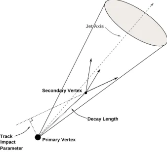
The SV0 tagging algorithm is a lifetime-based b-tagger which explicitly reconstructs secondary vertices from tracks associated with a jet. The operation of this tagging algorithm involves placing a cut on the signed decay length significance, L/σ(L), of the reconstructed secondary vertex. The sign of L/σ(L) is given by the sign of the projection of the decay length vector on the jet axis. An illustration of a SV0-tagged jet is shown in Fig. 1.
As input, the tagging algorithm is given a list of tracks associated to the calorimeter jet. The track-to- jet association is done using a∆R matching between the tracks and the jet axis. A track is not allowed to be associated to multiple jets, but only to the closest one. For this analysis, a cone size of∆R=0.4 was used. Only tracks in jets fulfilling the criteria listed in Table 1 are used in the secondary vertex fit. These tracks are referred to as SV0 tracks. The track selection criteria are slightly different to the selection criteria for the impact-parameter based taggers [3] as a result of the SV0-specific optimization.
Selection
pT >0.5 GeV
d0PV <2 mm
zPV0 sinθ <2 mm
σ(d0PV) <1 mm σ(zPV0 ) <5 mm
χ2/ndof <3
Number of Pixel hits ≥2 Number of SCT hits ≥4 Number of Pixel+SCT hits ≥7
Table 1: Track selection criteria used by the SV0 tagging algorithm, where d0PV and zPV0 denote the impact parameters of the track in the transverse plane and the longitudinal direction respectively. They are derived with respect to the reconstructed primary vertex. Theχ2/ndof is that of the track fit.
Using these SV0 tracks as input the SV0 algorithm starts by reconstructing two-track vertices signif- icantly displaced (in three dimensions) from the primary vertex. Tracks are considered for the two-track vertices if dca/σ(dca)>2.3, where dca/σ(dca)is the 3-dimensional impact parameter significance of the track in three dimensions with respect to the primary vertex. Furthermore, the sum of the impact
Primary Vertex
Jet Axis
Decay Length
Track Impact Parameter
Secondary Vertex
Figure 1: A secondary vertex with a significant decay length indicates the presence of a long-lived particle in the jet. The secondary vertex is reconstructed from tracks with a large impact parameter significance with respect to the primary vertex.
parameter significances of the two tracks has to be greater than 6.6. Two-track vertices must have a χ2<4.5 and be incompatible with the primary vertex by requiring the χ2 of the distance between the primary and secondary vertex, computed in three dimensions, to be greater than 6.25.
The algorithm then removes two-track vertices with a mass consistent with a Ks0meson, aΛ0baryon or a photon conversion. In addition, two-track vertices at a radius consistent with the radius of one of the three Pixel detector layers are removed, as these vertices likely originate from material interactions.
For each jet, the tracks in surviving two-track vertices are taken together and fitted to a single sec- ondary vertex. In an iterative process it removes the track with the largestχ2contribution to the common vertex until the fit probability of the vertex is greater than 0.001, the vertex mass is less than 6 GeV and the largest χ2 contribution from any one track is 7 or less. Finally it tries to re-incorporate the tracks failing the selections made during the formation of two-track vertices into the vertex fit.
4 Data Samples and Selections
The data are compared to non-diffractive minimum bias events generated withPYTHIA6.4.21 [4] using theMRST LO∗parton distribution functions [5]. To simulate the detector response, the generated events are processed through a GEANT4 [6] [7] simulation of the ATLAS detector, and then reconstructed and analyzed as the data.
Data Quality criteria have been applied for the Inner Detector tracking detectors and the calorimeters to ensure a proper functioning of these devices. The solenoid magnet was on through the entire period.
Events were selected from the Minimum bias stream. They are triggered by requiring at least one hit in any of the MBTS detectors in coincidence with a BPTX signal. The events are required to have exactly one reconstructed primary vertex containing at least ten tracks [8] to ensure a good primary vertex resolution. Events with additional primary vertices are allowed if they contain less than five tracks.
Jets are reconstructed from topological clusters [2] of energy in the calorimeter using the anti-kt
algorithm with size of 0.4 [9], and are required to have pT >20 GeV and |η|<1.8. The cut onη is motivated in [10]. The jets are calibrated [11] and a set of cleaning cuts is applied [12]. Furthermore they have to contain at least one track.
5 Displaced Vertices in Jets
As described in Section 3, the secondary vertex algorithm uses good-quality tracks associated to calorime- ter jets. For a good understanding of the tagging algorithm performance it is therefore of great importance to study this set of tracks closely, and to ensure that their properties are well modelled by the simulation.
Tracks with selection criteria very close to those used by the SV0 algorithm are studied elsewhere [10], and the agreement between data and simulation is found to be very good.
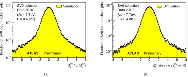
Figure 2 shows the signed impact parameter significance distributions with respect to the primary vertex in both the transverse and longitudinal plane for tracks fulfilling the selection criteria given in Table 1. The sign is defined using the jet direction measured by the calorimeters: it is positive if the angle between the jet direction and the line joining the primary vertex to the point of closest approach is less than 90◦, negative otherwise. The distributions are normalized to unit area to allow for shape com- parisons. There is good agreement between data and simulation. The data distribution is slightly wider which might point to residual misalignment. In the SV0 algorithm, only tracks with a 3D significance greater than 2.3 are used, i.e. preferentially those tracks in the tails of the significance distributions.
The following figures show properties of vertices which are reconstructed with the SV0 algorithm as described in Section 3. There are 856 jets in the data having a secondary vertex with a positive decay
PV) (d0
σ
PV / d0
-8 -6 -4 -2 0 2 4 6 8
Fraction of SV0 input tracks in jets
10-4
10-3
10-2
10-1 SV0 selection Data 2010
= 7 TeV, s (
-1) L = 0.4 nb
Simulation
ATLAS Preliminary
(a)
θ) sin
PV
(z0
σ θ / sin
PV
z0
-8 -6 -4 -2 0 2 4 6 8
Fraction of SV0 input tracks in jets
10-4
10-3
10-2
10-1 SV0 selection Data 2010
= 7 TeV, s (
-1) L = 0.4 nb
Simulation
ATLAS Preliminary
(b)
Figure 2: d0PV (a) and zPV0 sinθ (b) significance with respect to the reconstructed primary vertex for all SV0 tracks in jets. The data (solid markers) are compared to the simulation (histogram) of non-diffractive minimum bias events. The data and simulation distributions are both normalized to unit area to allow for shape comparisons.
length, and 427 of them fulfill L/σ(L)>7. The numbers expected from the same number of jets in simulated events are 788±15 and 382±7 vertices respectively (the uncertainty is statistical only). Thus there are approximately 10% more secondary vertices per jet in data than simulation. In the following all distributions of vertex properties are normalized to the number of jets in data before tagging unless stated otherwise. They are thus sensitive to the absolute number of secondary vertices reconstructed per jet.
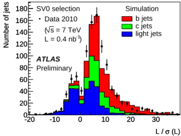
Figure 3 shows the signed decay length significance, L/σ(L), for all reconstructed secondary ver- tices. The shape of the distribution is well modelled by the simulation, both in the low decay length significance region which is dominated by background from c- and light jets and in the large decay length significance region where the sample is dominated by b-jets.
Figure 4 shows the number of tracks associated to the reconstructed secondary vertices with L/σ(L)>
0. There is a fair agreement between the number of tracks in data and simulation, but the average number of tracks associated to the vertices in data events is lower than in simulated events. In simulated events, where the components from b-, c- and light jets are shown separately, it is seen that the light jets are the dominant contribution to the two-track vertices. The disagreement observed in this bin could thus be caused by an underestimate of the amount of light jets with a secondary vertex in the simulation.
Figure 5 shows the impact parameter significance in the transverse and longitudinal directions of the tracks associated to the secondary vertices. The distributions are normalized to unit area to allow for shape comparisons. The data distribution is wider than that in simulated events. This is likely due to remaining residual data misalignments or imperfections in the material description of the Inner Detector that are still present at this early stage of the experiment.
Figure 6(a) shows the invariant mass, Mvtx, of the tracks associated to the reconstructed secondary vertices with L/σ(L)>0, while Fig. 6(b) shows this for all vertices with L/σ(L)>7. The agreement between data and simulation is generally good, but in both distributions there is an excess of data events in the low Mvtxregion. In simulated events it is seen that the b-jets tend to dominate at large Mvtxwhile the c- and light jets dominate at low Mvtx. The excess observed at low Mvtxis consistent with the simulation underestimating the amount of c- and light jets tagged by the SV0 algorithm. The fraction of jets in
the sample originating from b-quarks is greatly increased when selecting vertices with L/σ(L)>7, demonstrating the power of the SV0 tagging algorithm. In particular the b-jets clearly dominate for Mvtx>2 GeV.
σ (L) L /
-20 -10 0 10 20 30
Number of jets
0 20 40 60 80 100 120 140 160
180 SV0 selection Data 2010
= 7 TeV s (
-1) L = 0.4 nb
Simulation b jets c jets light jets
ATLAS Preliminary
σ (L) L /
-20 -10 0 10 20 30
Number of jets
0 20 40 60 80 100 120 140 160 180
Figure 3: The three-dimensional decay length significance, signed with respect to the calorimeter jet axis, for all secondary vertices reconstructed in data events (markers). The expectation from simulated events (histogram) for non-diffractive minimum bias events, normalized to the number of jets in the data, is superimposed.
Number of tracks used for secondary vertex
2 3 4 5 6 7 8 9
Number of jets
0 100 200 300 400 500
Number of tracks used for secondary vertex
2 3 4 5 6 7 8 9
Number of jets
0 100 200 300 400
500 SV0 selection
Data 2010
-1) = 7 TeV, L = 0.4 nb s
( Simulation
b jets c jets light jets
ATLAS Preliminary
Number of tracks used for secondary vertex
2 3 4 5 6 7 8 9
Number of jets
0 100 200 300 400 500
Figure 4: The number of tracks in secondary vertices. The expectation from simulated events (histogram) for non-diffractive minimum bias events, normalized to the number of jets in the data, is superimposed.
6 Conclusions
In this note, data-to-simulation comparisons of some of the quantities relevant for the secondary vertex tagging algorithm SV0 have been presented. The properties of the reconstructed secondary vertices are found to be in reasonable agreement with the expectations from simulated events. In particular in the regions that are expected to be dominated by b-jets the data agree well with the MC expectation.
PV) (d0
σ
PV / d0
-8 -6 -4 -2 0 2 4 6 8
Fraction of SV0 input tracks in jets
0 0.02 0.04 0.06 0.08 0.1 0.12
0.14 SV0 selection Data 2010
= 7 TeV, s (
-1) L = 0.4 nb
Simulation
ATLAS
(a)
θ) sin
PV
(z0
σ θ / sin
PV
z0
-8 -6 -4 -2 0 2 4 6 8
Fraction of SV0 input tracks in jets
0 0.02 0.04 0.06 0.08 0.1 0.12 0.14
0.16 SV0 selection
Data 2010 = 7 TeV, s (
-1) L = 0.4 nb
Simulation
ATLAS
(b)
Figure 5: d0PV (a) and zPV0 sinθ (b) distributions for tracks in secondary vertices. The expectation from simulated events (histogram) for non-diffractive minimum bias events is superimposed. The plots are normalized to unit area to allow shape comparisons.
[GeV]
mvtx
0 1 2 3 4 5 6
Number of jets
0 20 40 60 80 100 120 140 160 180 200 220
[GeV]
mvtx
0 1 2 3 4 5 6
Number of jets
0 20 40 60 80 100 120 140 160 180 200
220 SV0 selection
Data 2010
-1) = 7 TeV, L = 0.4 nb s
( Simulation
b jets c jets light jets
ATLAS Preliminary
[GeV]
mvtx
0 1 2 3 4 5 6
Number of jets
0 20 40 60 80 100 120 140 160 180 200 220
(a)
[GeV]
mvtx
0 1 2 3 4 5 6
Number of jets
0 10 20 30 40 50 60
[GeV]
mvtx
0 1 2 3 4 5 6
Number of jets
0 10 20 30 40 50
60 SV0 selection
Data 2010
-1) = 7 TeV, L = 0.4 nb s
( Simulation
b jets c jets light jets
ATLAS Preliminary
[GeV]
mvtx
0 1 2 3 4 5 6
Number of jets
0 10 20 30 40 50 60
(b)
Figure 6: The vertex mass distribution for all secondary vertices in data with positive decay length (a) and with a decay length significance greater than 7 (b). The expectation from simulated events, normalized to the number of jets in the data, is superimposed.
References
[1] The ATLAS Collaboration, Performance of the ATLAS Secondary Vertex b-tagging Algorithm in 900 GeV Collision Data, ATLAS-CONF-2010-004, March, 2010.
[2] G. Aad et al., The ATLAS Experiment at the CERN Large Hadron Collider, JINST 3 (2008) S08003.
[3] The ATLAS Collaboration, Expected performance of the ATLAS experiment: Detector, Trigger and Physics, Volume 1, CERN-OPEN-2008-020, December, 2008.
[4] T. Sjostrand, S. Mrenna, and P. Z. Skands, PYTHIA 6.4 Physics and Manual, JHEP 05 (2006) 026.
[5] A. Sherstnev and R. S. Thorne, Parton Distributions for LO Generators, Eur. Phys. J. C55 (2008) 553–575.
[6] GEANT4 Collaboration, S. Agostinelli et al., GEANT4: A simulation toolkit, Nucl. Instrum. Meth.
A506 (2003) 250–303.
[7] The ATLAS Collaboration, The ATLAS Simulation Infrastructure, Arxiv:1005.4568v1, May, 2010.
[8] G. Piacquadio, K. Prokofiev, and A. Wildauer, Primary vertex reconstruction in the ATLAS experiment at LHC, J. Phys. Conf. Ser. 119 (2008) 032033.
[9] M. Cacciari, G. P. Salam, and G. Soyez, The anti-k(t) jet clustering algorithm, JHEP 04 (2008) 063.
[10] The ATLAS Collaboration, Tracking studies for b-tagging with 7 TeV collision data with the ATLAS detector, ATLAS-CONF-2010-040, May, 2010.
[11] The ATLAS Collaboration, Observation of Energetic Jets in pp Collisions at√s = 7 TeV using the ATLAS Experiment at the LHC, ATLAS-CONF-2010-043, May, 2010.
[12] The ATLAS Collaboration, Data-Quality Requirements and Event Cleaning for Jets and Missing Transverse Energy Reconstruction with the ATLAS Detector in Proton-Proton Collisions at a Center-of-Mass Energy of√
s = 7 TeV, ATLAS-CONF-2010-038, May, 2010.