ATLAS NOTE ATLAS-CONF-2015-042

A TLAS-CONF-2015-042 31 August 2015

ATLAS NOTE

ATLAS-CONF-2015-042

31st August 2015

Search for New Phenomena in Dijet Mass and Angular Distributions with the ATLAS Detector at √

s = 13 TeV

The ATLAS Collaboration

Abstract

This note describes a search for pairs of jets (dijets) produced by phenomena beyond the Standard Model in 80 pb

of proton-proton collisions with a centre-of-mass energy of

√ s = 13 TeV recorded by the ATLAS detector at the Large Hadron Collider. We exam- ine the distribution of the invariant mass of the two leading jets for local excesses atop a data-driven estimate of the smoothly-falling distribution predicted by the Standard Model.

We also compare the data to a Monte Carlo simulation of the Standard Model using the distribution of an angular variable, χ, derived from the rapidity of the two jets. Both distri- butions lack evidence for anomalous phenomena. We exclude Quantum Black Holes with masses below 6.8 TeV or 6.5 TeV in two benchmark scenarios. We also set 95% C.L. upper limits on the cross section for new processes that would produce a Gaussian contribution to the dijet mass distribution. We exclude Gaussian contributions with e ff ective cross sections ranging from approximately 0.4–2 pb below 2 TeV to 0.05–0.09 pb above 4 TeV.

© 2015 CERN for the benefit of the ATLAS Collaboration.

Reproduction of this article or parts of it is allowed as specified in the CC-BY-3.0 license.

1 Introduction

When a particle collider increases its collision energy, it may cross beyond a threshold where new phe- nomena begin to produce observable e ff ects. For example, the energy may become su ffi ciently high to reveal the substructure of the colliding particles, or to directly produce particles that could not be produced at lower energies. The Large Hadron Collider (LHC) at CERN has recently increased the centre-of-mass energy of its proton-proton collisions from √

s = 8 TeV to √

s = 13 TeV, opening a new energy regime to observation.

In order to singly produce new particles in LHC collisions, the particles must interact with the constituent partons within the proton. This in turn means that the new particles can also decay to partons. Often in models of beyond the Standard Model (BSM) phenomena, these decays dominate.

The partons shower and hadronize, creating collimated jets of particles carrying approximately the four- momenta of the original partons. The total production rates for two-jet (dijet) BSM signals can be large, allowing searches for anomalous dijet production to test for such signals with a relatively small data sample, even at masses that involve significant fractions of the total hadron collision energy.

Prior searches of dijet distributions at hadron colliders from the SPS, Tevatron, and the √

s = 7–8 TeV LHC [1–17] did not observe BSM phenomena. This note presents a search for BSM phenomena using 80 pb

of collision data recorded by the ATLAS detector at the LHC. Analyses are performed on the distributions of the dijet invariant mass, m

, and of a variable derived from the angular separation of the two jets, χ, defined below.

In the Standard Model of particle physics, hadron collisions produce jet pairs primarily via 2 → 2 parton scattering processes governed by Quantum Chromodynamics (QCD). Far above the confinement scale of QCD (≈ 1 GeV), jets emerge from collisions with large momenta, p

, transverse to the direction of the incident partons. Most dijet production, however, occurs at small angles θ

with respect to the direction of the incident partons in the parton-parton centre-of-mass frame1, due to t-channel poles in the cross sections for the dominant scattering processes. Many theories of BSM physics predict additional dijet production with a significant population of jets produced at large angles with respect to the beam (for reviews see Refs. [18, 19]). For the data analysed in this note, QCD predicts an m

distribution that is smoothly falling, without a characteristic mass scale or other features. In contrast, new states decaying to two jets may introduce localized excesses in the mass distribution if the states have su ffi ciently narrow width. The search performed in this note exploits these differences in the χ and m

distributions.

As is common, we define a rapidity y =

ln

z

for each of the outgoing partons, where E is its energy and p

is the component of its momentum along the beam pipe 2 . Each incoming parton carries a fraction (Bjorken x) of the momentum of its proton. A momentum imbalance between the two partons boosts the centre-of-mass frame of the collision relative to the detector frame along the z direction. The boost from the laboratory to the centre-of-mass frame along the z direction is y

=

ln (x/x

) =

( y

+ y

), where x and x

are the fractions of the proton momentum carried by each parton and y

and y

are rapidities of the outgoing partons in the detector frame. This boost is zero when both partons carry the same momentum

1

Since, experimentally, the two partons cannot be distinguished, θ

is always taken between 0 and π/2.

2

ATLAS uses a right-handed coordinate system with its origin at the nominal interaction point (IP) in the centre of the detector and the z-axis along the beam pipe. The x-axis points from the IP to the centre of the LHC ring, and the y-axis points upwards. Cylindrical coordinates (r, φ) are used in the transverse plane, φ being the azimuthal angle around the z-axis. The pseudorapidity is defined in terms of the polar angle θ as η = −ln tan(θ/2). It is equivalent to the rapidity for massless

q

(x = x

). Di ff erences in two rapidities are invariant under Lorentz boosts along the z direction. Therefore the following function of the rapidity difference y

=

(y

− y

) between the two outgoing jets,

χ = e

∼ 1 + cos θ

1 − cos θ

(1)

is the same in the detector frame as in the partonic centre-of-mass frame. In the centre-of-mass frame, the two partons have rapidity ±y

.

The variable χ is constructed such that in the limit of massless parton scattering, and when only t-channel scattering contributes to the partonic cross section, the shape of the distribution of χ will be approximately independent of the two-parton invariant mass. The shapes of the observed χ distributions are distorted from the χ distributions at parton-level by the non-uniform parton momentum distributions as a function of x and x

. Restricting the size of y

restricts the ranges of x and x

and reduces these distortions.

2 ATLAS Detector

The ATLAS experiment [20] at the LHC is a multi-purpose particle detector with a forward-backward symmetric cylindrical geometry with layers of tracking, calorimeter, and muon detectors over nearly the entire solid angle around the pp collision point. High-p

hadronic jets are measured using finely seg- mented hadronic and electromagnetic calorimeters. A steel / scintillator-tile calorimeter provides hadronic energy measurements for the pseudorapidity range (|η | < 1.7). A lead/liquid-argon (LAr) calorimeter provides electromagnetic (EM) energy measurements with higher granularity. The end-cap and forward regions are instrumented with LAr calorimeters for both EM and hadronic energy measurements up to

|η | = 4.9. A muon spectrometer surrounds the calorimeters. A first-level trigger is implemented in hard- ware and uses a subset of the detector information to reduce the accepted rate to 100 kHz. This is followed by a software-based trigger that reduces the average recorded collision rate to 1 kHz.

3 Data Selection

The analysis described in this note uses proton–proton collision data at 13 TeV centre-of-mass energy recorded in August 2015. Collision events are recorded using a trigger requiring the presence of at least one jet reconstructed in the software trigger with a p

of at least 360 GeV. The dataset does not include earlier data due to an inefficiency in the triggering of very high energy objects.

Groups of contiguous calorimeter cells (topological clusters) are formed based on the significance of the energy deposit over calorimeter noise [21]. These are clustered into jets using the anti-k

algorithm [22, 23] with distance parameter R = 0.4. Jet four-momenta are computed summing over the four-momenta of the topological clusters that comprise the jet, treating each cluster as a four-vector with zero mass.

These four-momenta are calibrated for the response to incident hadrons using the procedures described in Refs. [24, 25]. The agreement between data and simulation is further improved by the application of jet- wise calibration constants obtained at lower collision energies with in situ techniques [26] and validated for use at 13 TeV [27].

Events containing at least two jets are selected for offline analysis if the p

of the leading-p

jet is greater

than 410 GeV and the p

of the subleading-p

jet is greater than 50 GeV. The requirement on leading jet

p

ensures a trigger e ffi ciency of at least 99.5 % for collisions with | y

| < 1.7. Events are discarded from the search if either of the two leading jets, or a third jet with p

> 50 GeV, are poorly measured or have a topology compatible with non-collision background or calorimeter noise [28].

4 Simulated Collisions

For this search, events have been simulated for QCD processes with P ythia 8 [29] using the A14 [30]

underlying event tune and the NNPDF2.3 LO [31] PDFs. Detector effects are simulated using Geant4 within the ATLAS software infrastructure [32, 33]. The same software used to reconstruct data was used for the simulated events.

Pythia 8 calculations use matrix elements which are leading order (LO) in the QCD coupling constant with simulation of higher-order contributions partially included in the parton shower (PS) modeling. P y - thia 8 also includes modeling of hadronization e ff ects. We reweight the distributions of events predicted by Pythia 8 to the next-to-leading-order (NLO) cross-section predictions of NLOJET++ [34–36] using m

- and χ-dependent correction factors,

k ( χ, m

) = σ

( χ, m

)

σ

( χ, m

)

.

Here σ

is the cross-section obtained in Pythia 8 with hadronization corrections turned off. The correction factors modify the shape of the χ distributions at the level of 15% at low values of χ and high values of m

. The correction is 5% or less at the highest values of χ. The P ythia 8 predictions also omit electroweak effects. We include these as additional m

- and χ-dependent correction factors [37]. The correction factors are unity at low m

and differ from unity by up to 3% in the m

> 3.4 TeV region.

5 Resonance Analysis

The search in the m

distribution is performed using events with | y

| < 0.6 ( χ < 3.3). The requirement on | y

| reduces the background to resonant BSM physics from QCD processes. To avoid kinematic bias from the selections described in Section 3, the search is confined to m

> 1100 GeV.

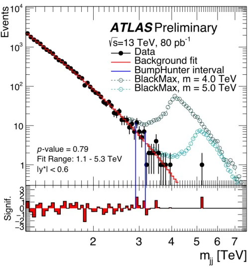
Figure 1 shows the observed m

distribution for the resonance analysis. The bin width varies with mass and is chosen to approximate the m

resolution as derived from the simulation of QCD processes. The largest value of m

measured is 5.2 TeV. ATLAS, CMS, and CDF dijet searches [4, 6, 11, 12, 14] have found that an ansatz of the form

f ( z) = p

(1 − z)

z

(2) where z ≡ m

/ √

s, and p

are chosen by the fit, describes dijet mass distributions observed at lower

collision energies. The ansatz also describes leading and next-to-leading order simulations of QCD dijet

production. The Standard Model background to the present analysis is estimated by a fit to the entire

observed m

distribution with the same function. While providing data at lower m

values, the obser-

vations at lower collision energies involved larger statistics and wider ranges of mass than are available

in the present 13 TeV ATLAS data, and all four parameters were needed in order to obtain a satisfactory

[TeV]

Reconstructed m

2 3 4 5 6 7

Events

1 10 10

10

10

|y*| < 0.6

Fit Range: 1.1 - 5.3 TeV -value = 0.79 p

[TeV]

m jj

2 3 4 5 6 7

Signif.

3

− 2

− − 01 23 1

ATLAS Preliminary

=13 TeV, 80 pb -1

s Data

Background fit

BumpHunter interval BlackMax, m = 4.0 TeV BlackMax, m = 5.0 TeV

Figure 1: The dijet mass distribution (filled points) for events in with |y

| < 0.6 and p

> 410 (50) GeV for the leading (subleading) jets fitted with a function described by Eq. 2 (solid line) discussed in the text. Predictions from B lack M ax for two Quantum Black Hole signals are shown above the fit, normalized to the predicted cross section.

The vertical lines indicate the most discrepant interval identified by the B ump H unter algorithm. The bottom panel shows the bin-by-bin significance of the data-fit di ff erence, considering statistical uncertainties only.

p

set to zero will remain a good description of the m

distribution until substantially more data are col- lected, and thus the log z term is removed from the fit. To avoid bias from a BSM process that contributes in a single, contiguous range of bins, any such range is automatically excluded from the fit if an excess in those bins decreases the fit probability below 0.01.

The function in Eq. 2 is fit to this distribution with a probability of 0.45. The result is also shown in the figure. The bottom panel of the figure shows the significances of bin by bin differences between the data and the fit. These Gaussian significances are calculated from the Poisson probability. The significance takes statistical uncertainties but no systematic uncertainties into account.

We search for statistical evidence of any localized excess in this distribution using the B ump H unter

algorithm [38, 39]. The algorithm operates on the binned m

distribution, comparing the data with the

fitted background estimate in all possible mass intervals, up to half the mass range spanned by the data.

For each interval in the scan, it computes the significance of any excess found. The algorithm identifies the interval 2.91–3.17 TeV, indicated by the two vertical lines in Figure 1, as the single most discrepant interval. The significance of the outcome is evaluated using the ensemble of possible outcomes across all intervals scanned, by repeating the algorithm on pseudo-data drawn from the background fit. Before including systematic uncertainties, the probability (p-value) of observing a background fluctuation at least as significant as the above, anywhere in the distribution, is 0.78. There is no evidence for a localized contribution to the distribution from BSM physics.

6 Angular Analysis

The search in χ distributions is performed using dijet events with | y

| < 1.7 (i.e. χ < 30.0) and | y

| <

1.1. To avoid kinematic bias from the selections described in Section 3, the search is confined to m

>

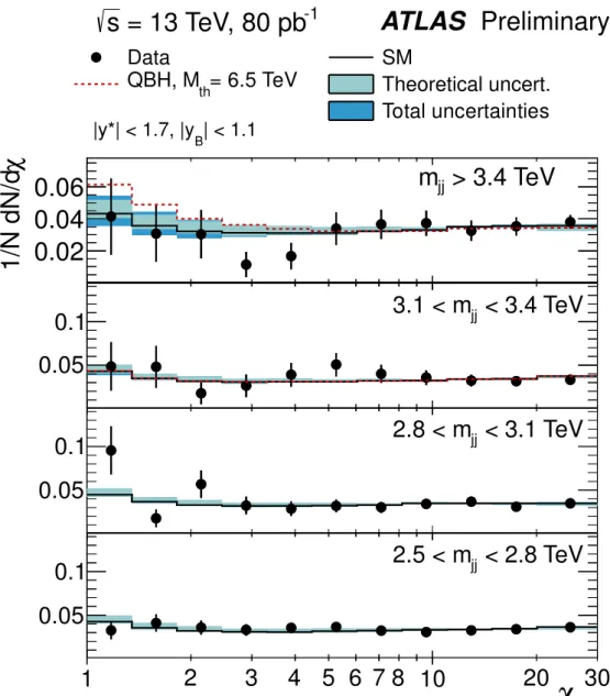
2500 GeV. Figure 2 shows the χ distributions of the data in the angular analysis in different m

ranges.

The highest m

measured is 6.9 TeV. In the analysis, the Standard Model prediction in each m

range is normalised to match the integral of the data in that range. The shapes of the χ distributions in the figure are compared to data after normalising both to unit area. The theoretical uncertainties and the total uncertainties are displayed as shaded bands around the Standard Model prediction.

The C L

-technique [40, 41] is used to test the compatibility of the χ distribution with the Standard Model

prediction and with a quantum black hole BSM signal (see below). The top panel in Figure 2 shows the

data in the m

range used for this test. The data prefer the background-only hypothesis, with a C L

statistic of 0.50 for the highest m

range. The χ

probability for the observed data given the Standard

Model prediction is 0.57.

χ

1 2 3 4 5 6 7 8 10 20 30

0.05

0.1 2.5 < m _jj < 2.8 TeV

0.05

0.1 2.8 < m _jj < 3.1 TeV

0.05

0.1 3.1 < m _jj < 3.4 TeV

χ

1/N dN/d 0.02 0.04

0.06 m _jj > 3.4 TeV

Data SM

= 6.5 TeV

QBH, M

Theoretical uncert.

Total uncertainties

| < 1.1

|y*| < 1.7, |y

ATLAS Preliminary = 13 TeV, 80 pb -1

s

Figure 2: Distributions of the dijet angular variable χ in di ff erent regions of the dijet invariant mass m

for events

with |y

| < 1.7, | y

| < 1.1 and p

> 410 (50) GeV for the leading (subleading) jets. Shown are the data

(points), corrected P ythia 8 predictions (solid lines), and one prediction from the QBH generator for the Quantum

Black Hole model discussed in the text. The theoretical uncertainties and the total theoretical and experimental

uncertainties are displayed as shaded bands around the Standard Model prediction.

7 Signal Models

As the measured m

and χ distributions do not deviate significantly from expectation, we use that data to constrain models that predict excesses in the distributions. While dijet resonances are predicted in many models of BSM physics, in this initial 13 TeV result we focus on a particularly high-rate scenario where gravity can propagate in extra dimensions [19, 42–45] and thus low-entropy black holes can be produced.

Models with extra dimensions, such as the Arkani-Hamed–Dimopoulous–Dvali (ADD) model [46, 47], solve the mass hierarchy problem of the Standard Model by lowering the fundamental scale of quantum gravity, M

to a few TeV. Consequently, the LHC could produce quantum black holes with masses at or above M

[48, 49]. A Quantum Black Hole produced near M

would evaporate faster than it thermalizes, decaying into a few particles rather than high-multiplicity final states [44, 45, 50]. Such a signal would appear as a local excess over the m

distribution near the threshold mass, M

, and would fall exponentially at higher masses. In this note, Quantum Black Hole production and decay to two jets is simulated using both the QBH generator [51] and the B lack M ax generator [50], assuming an ADD scenario with M

= M

and n = 6, as in Ref. [14].

The two generators make different assumptions about the physics of black hole production and decay.

Black holes decay thermally in B lack M ax , while the decay products of the QBH generator are dictated by particle conservation principles. Moreover, the QBH generator includes the e ff ects of spin while the BlackMax generator does not.

The acceptance times e ffi ciency in the resonance analysis for a Quantum Black Hole with mass 6.5 TeV is 54% for the QBH generator and 53% for the B lack M ax generator. For the angular analysis, the corres- ponding acceptance times efficiency is 92% for the QBH generator and 91% for the B lack M ax generator.

For both Quantum Black Hole generators, the CTEQ6L1 [52] PDFs are used instead of NNPDF2.3 LO PDFs, to ensure good behavior at extreme values of Bjorken x.

Subsequent to parton-level calculations, the Quantum Black Hole models are simulated in an identical manner to QCD processes, using the same parameters for non-perturbative corrections.

Results are also provided on the cross section, σ, times acceptance, A, times branching ratio, BR, to two jets of a hypothetical signal that produces a Gaussian contribution to the observed m

distribution.

For su ffi ciently narrow resonances, these results may be used to set limits on BSM models beyond those

considered explicitly in this note. Such limits should be used when PDF and nonperturbative effects

can be safely truncated or neglected and, after applying the kinematic selection criteria of the resonance

analysis, the distribution of m

for a signal approaches a Gaussian distribution. The resulting limit will

be conservative at high masses with respect to the limits obtained with full benchmark templates. BSM

models with an intrinsic width much smaller than 5% should be compared to the results with width

equal to the experimental resolution. For models with a larger width after detector e ff ects, the limit that

best matches their width should be used. More detailed instructions can be found in Appendix A of

Ref. [14].

8 Systematic Uncertainties

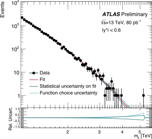
In the resonance analysis, systematic uncertainties on the estimate of the background to the search arise from imperfect knowledge of the shape of the m

distribution. To account for the statistical uncertainty on the fitted parameters in Eq. 2, a large number of pseudo-experiments are performed, fitting pseudo-data drawn via Poisson fluctuations around the nominal background model. The uncertainty on the background prediction in each m

bin is taken to be the root mean square of the function value in that bin for all pseudo-experiments. To account for the choice of function used in the fit, a parameterization with one additional degree of freedom, p

, is compared to the nominal fit. Fig. 3 shows these two contributions to the uncertainty on the background prediction.

2 3 4 5

Events

1 10 10

10

10

|y*| < 0.6

Data Fit

Statistical uncertainty on fit Function choice uncertainty

=13 TeV, 80 pb

s

ATLAS Preliminary

[TeV]

m

2 3 4 5

Rel. Uncert.

1

− 0.5

−0.51.501

Figure 3: The dijet mass distribution (points) for events with |y

| < 0.6 and p

> 410 (50) GeV for the lead- ing (subleading) jets fitted with a function described by Eq. 2 (solid line). The light and dark cyan lines depict variations of the background prediction from the statistical uncertainty on the fitted parameters and from the uncer- tainty due to the choice of function, as described in the text. The bottom panel depicts the relative uncertainty from each source.

In the angular analysis, theoretical uncertainties on simulations of the χ distributions of QCD processes

are estimated as described in Ref. [17]. The resonance search does not estimate the background using

simulated collisions and thus it is not a ff ected by uncertainties on simulations of QCD processes. The effect on the Pythia 8 QCD prediction of varying the PDFs is estimated using NLOJET++ with three di ff erent PDF sets: CT10, MSTW2008 [53] and NNPDF23 [54]. As the choice of PDF largely a ff ects the total cross section rather than the shape of the χ distributions, these uncertainties are negligible (< 1%). The uncertainty due to the choice of renormalization and factorization scales was estimated using NLOJET ++ by varying each independently up and down by a factor two. The resulting uncertainty, taken as the envelope of the variations in the normalized χ distributions, depends on both m

and χ, rising to 20% at the smallest χ values at high m

values. The uncertainties due to limited statistics in the simulation of the NLO corrections are less than 1%. The dominant experimental uncertainty on the predictions of the χ distributions is the jet energy scale uncertainty. It is derived from 8 TeV data and complemented by additional uncertainties derived using 13 TeV data to account for differences in the calibration and detector conditions [27]. The impact of this uncertainty is at most 9%.

The following systematic uncertainties are included in setting limits on the Quantum Black Hole models:

statistical uncertainties, jet energy scale (up to 10%), and PDF and uncertainties due to higher-order corrections (1%). The impact of the uncertainty on the jet energy resolution is negligible. The uncertainty on the integrated luminosity is ±9%. It is derived, following a methodology similar to that detailed in Ref. [55], from a preliminary calibration of the luminosity scale using a pair of x-y beam-separation scans performed in June 2015.

9 Limits

Starting from the m

distribution obtained by the resonance analysis, a Bayesian method [12] is applied to the data and QBH or BlackMax simulation at a series of discrete masses to set a 95% credibility- level upper limit on the cross section times acceptance for the two types of signals. The method uses a prior constant in signal strength and Gaussian priors for nuisance parameters corresponding to systematic uncertainties. The limit is interpolated between the discrete masses to create a curve continuous in black hole mass.

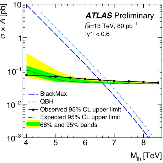
Figure 4 shows the limit as a function of the Quantum Black Hole mass for the QBH and B lack M ax generators. From these limits, Quantum Black Holes in the n = 6, M

= M

ADD scenario simulated with the QBH generator with M

below 6.8 TeV are excluded at 95% credibility level. Signals pro- duced by the B lack M ax generator are excluded below 6.5 TeV. These supercede the exclusions below 5.66 TeV (5.62 TeV) on QBH (BlackMax) signals set by the ATLAS Collaboration using dijet events at

√ s = 8 TeV [14]. A search performed by the CMS Collaboration for Quantum Black Holes yielded limits in the range of 5.0–6.3 TeV, for n = 1–6 and di ff erent model assumptions [56].

Starting from the χ distribution obtained by the angular analysis, the C L

technique is applied between the Standard Model and the QBH or B lack M ax simulation, using the asymptotic approximation [57] and a one-sided profile likelihood ratio, to set a 95% confidence-level upper limits on Quantum Black Hole production. The validity of the asymptotic approximation was confirmed using toy simulations. The limits are calculated in the most sensitive region, m

> 3.4 TeV.

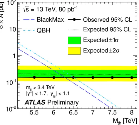
Figure 5 shows the limit from the angular analysis as a function of the Quantum Black Hole threshold

mass for the n = 6, M

= M

ADD scenario simulated with the QBH and B lack M ax generators. These

results exclude black holes simulated with the QBH generator with M

below 6.5 TeV at 95% C.L. The

[TeV]

M th

4 5 6 7 8

[pb] A × σ

− 3

10

− 2

10

− 1

10 1 10

BlackMax QBH

Observed 95% CL upper limit Expected 95% CL upper limit 68% and 95% bands

s ^-1

ATLAS Preliminary

=13 TeV, 80 pb

|y*| < 0.6

Figure 4: Observed (filled circles) and expected 95% credibility-level upper limits (dotted line) on the cross section,

σ, times acceptance, A, for Quantum Black Holes as a function of particle mass, obtained from the m

distribution.

The green and yellow bands represent the 68% and 95% contours of the expected limit. The dashed and dotted- dashed curves are the theoretical predictions of σ × A for the B lack M ax and QBH generators. The observed (expected) mass limit occurs at the crossing of each σ × A curve with the observed (expected) 95% credibility-level upper limit curve.

corresponding exclusion for predictions of the B lack M ax Generator is 6.4 TeV. The results are consistent with the resonance analysis.

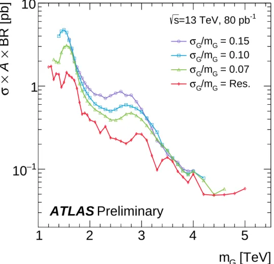
Figure 6 shows limits on the Gaussian contributions to the observed m

distribution obtained for four

different widths, from a width equal to the detector mass resolution to 15% of the mean mass of the

Gaussian distribution. The mass resolution is 2% at a mass of 4 TeV. As the width increases, the localized

excess becomes less distinct, and the limit weakens, accompanied by a decrease in the impact of statistical

fluctuations as the expected signal contribution is distributed across more bins. For intrinsically narrow

resonances, which would contribute a Gaussian distribution of width equal to the detector mass resolution,

we exclude e ff ective cross sections ranging from approximately 2 pb below 2 TeV to 0.05 pb above

4 TeV.

[TeV]

M th

5.5 6 6.5 7 7.5 8

[pb] A × σ

10 -2

10 -1

1 10 10 2

Observed 95% CL Expected 95% CL

1 σ Expected ±

2 σ Expected ± BlackMax

QBH

= 13 TeV, 80 pb -1

s

ATLAS Preliminary

> 3.4 TeV m

| < 1.1

|y*| < 1.7, |y

Figure 5: Observed (filled circles) and expected 95% confidence-level upper limits (dotted line) on the cross section,

σ, times acceptance, A for Quantum Black Holes as a function of particle mass, obtained from the χ distribution.

The green and yellow bands represent the 68% and 95% contours of the expected limit. The dashed and dotted-

dashed curves are the theoretical predictions of σ × A for the B lack M ax and QBH generators. The observed

(expected) mass limit occurs at the crossing of each σ × A curve with the observed (expected) 95% credibility-level

upper limit curve.

[TeV]

m G

1 2 3 4 5

BR [pb] × A × σ

− 1

10 1 10

ATLAS Preliminary

=13 TeV, 80 pb -1

s

= 0.15 /m G

σ G

= 0.10 /m G

σ G

= 0.07 /m G

σ G

= Res.

/m G

σ G

Figure 6: The 95% credibility-level upper limits obtained in the resonance analysis on cross section, σ, times

acceptance, A, times branching ratio, BR, to two jets for a hypothetical signal that produces a Gaussian contribution

to the observed m

distribution, as a function of the mean mass of the Gaussian distribution, m

. Limits are

obtained for four di ff erent widths, from a width equal to the detector mass resolution (“Res.”) to 15% of the mean

mass of the Gaussian distribution.

10 Conclusion

No evidence for phenomena beyond the Standard Model was uncovered in this search using dijets events in 80 pb

of proton-proton collisions with a centre-of-mass energy of √

s = 13 TeV recorded by the ATLAS detector at the Large Hadron Collider. The dijet invariant mass distribution exhibits no significant local excesses atop a data-driven estimate of the smoothly-falling distribution predicted by the Standard Model. The distribution of the angular variable χ also agrees with a Monte Carlo simulation of the Standard Model. In an ADD scenario with n = 6 and M

= M

, we exclude Quantum Black Holes predicted by the QBH generator with M

below 6.8 TeV (6.5 TeV) at 95% C.L. using the resonance (angular) analysis. The exclusions for the B lack M ax generator are 6.5 TeV (6.4 TeV). We also set 95%

C.L. upper limits on the cross section for new processes that would produce a Gaussian contribution to

the dijet mass distribution. We exclude Gaussian contributions with effective cross sections ranging from

approximately 0.4–5 pb below 2 TeV to 0.05–0.09 pb above 4 TeV.

Appendix

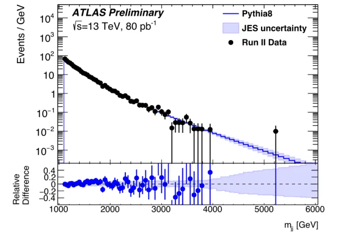
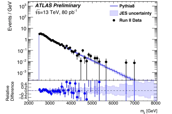
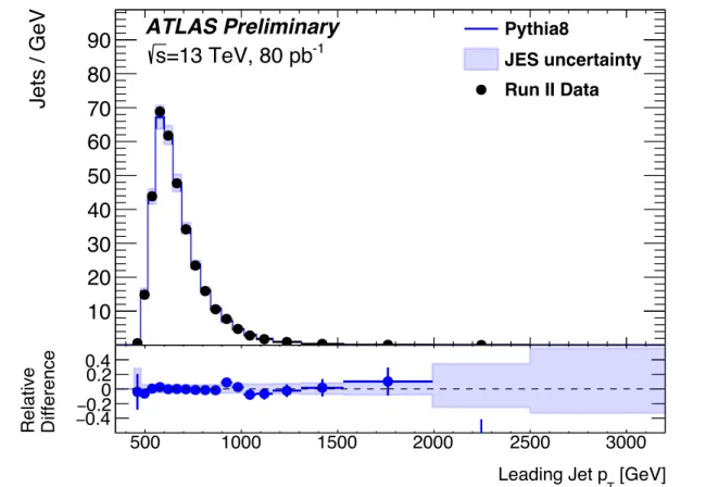
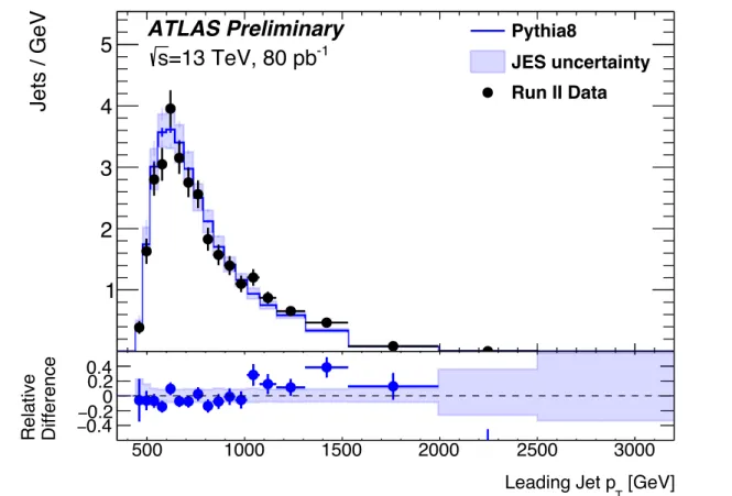
Figures 7-12 show the m

distributions and the p

distributions for the leading and subleading jets in events selected by the resonance analysis or the angular analysis. The figures also show the P ythia 8 simulation of QCD processes overlaid. The shaded band indicates the experimental uncertainty on the jet energy scale calibration. The NLO and electroweak correction factors, described in the text, are not applied to the simulation in these figures.

Figure 13 displays the highest mass dijet event found by the resonance analysis. Figure 14 displays the highest mass dijet event found by the angular analysis.

[GeV]

m

1000 2000 3000 4000 5000 6000

Events / GeV

−3

10

−2

10

−1

10 1 10 10

10

10

^Pythia8

JES uncertainty Run II Data

ATLAS Preliminary

=13 TeV, 80 pb

s

[GeV]

m

1000 2000 3000 4000 5000 6000

Difference Relative 0.4 − 0.2 − 0 0.2 0.4

Figure 7: The observed m

distribution obtained with the resonance analysis selection of events with |y

| < 0.6

and p

> 410 (50) GeV for the leading (subleading) jets. The distribution predicted by P ythia 8 simulation of

QCD processes is overlaid. The NLO and electroweak correction factors, described in the text, are not applied

to the simulation in this figure. The shaded band indicates the experimental uncertainty on the jet energy scale

calibration. Theoretical uncertainties are not depicted.

[GeV]

m

2000 3000 4000 5000 6000 7000 8000

Events / GeV

−3

10

−2

10

−1

10 1 10 10

10

^Pythia8

JES uncertainty Run II Data

ATLAS Preliminary

=13 TeV, 80 pb

s

[GeV]

m

2000 3000 4000 5000 6000 7000 8000

Difference Relative 0.4 − 0.2 − 0 0.2 0.4

Figure 8: The observed m

distribution obtained in the angular analysis selection of events with | y

| < 1.7,

| y

| < 1.1 and p

> 410 (50) GeV for the leading (subleading) jets. The distribution predicted by P ythia 8

simulation of QCD processes is overlaid. The NLO and electroweak correction factors, described in the text, are

not applied to the simulation in this figure. The shaded band indicates the experimental uncertainty on the jet energy

scale calibration. Theoretical uncertainties are not depicted.

[GeV]

Leading Jet p

500 1000 1500 2000 2500 3000

Jets / GeV

10 20 30 40 50 60 70 80

90 ^Pythia8

JES uncertainty Run II Data

ATLAS Preliminary

=13 TeV, 80 pb

s

[GeV]

Leading Jet p

500 1000 1500 2000 2500 3000

Difference Relative 0.4 − 0.2 − 0 0.2 0.4

Figure 9: The observed p

distribution of the leading jet, obtained with the resonance analysis selection of events

with |y

| < 0.6 and p

> 50 GeV for the subleading jet. The distribution predicted by P ythia 8 simulation of

QCD processes is overlaid. The NLO and electroweak correction factors, described in the text, are not applied

to the simulation in this figure. The shaded band indicates the experimental uncertainty on the jet energy scale

calibration. Theoretical uncertainties are not depicted.

[GeV]

Leading Jet p

500 1000 1500 2000 2500 3000

Jets / GeV

1 2 3 4

5 ^Pythia8

JES uncertainty Run II Data

ATLAS Preliminary

=13 TeV, 80 pb

s

[GeV]

Leading Jet p

500 1000 1500 2000 2500 3000

Difference Relative 0.4 − 0.2 − 0 0.2 0.4

Figure 10: The observed p

distribution of the leading jet, obtained with the angular analysis selection of events

with |y

| < 1.7, |y

| < 1.1, and p

> 50 GeV for the subleading jet. The distribution predicted by P ythia 8

simulation of QCD processes is overlaid. The NLO and electroweak correction factors, described in the text, are

not applied to the simulation in this figure. The shaded band indicates the experimental uncertainty on the jet energy

scale calibration. Theoretical uncertainties are not depicted.

[GeV]

Subleading Jet p

500 1000 1500 2000 2500 3000

Jets / GeV

20 40 60 80 100

Pythia8

JES uncertainty Run II Data

ATLAS Preliminary

=13 TeV, 80 pb

s

[GeV]

Subleading Jet p

500 1000 1500 2000 2500 3000

Difference Relative 0.4 − 0.2 − 0 0.2 0.4

Figure 11: The observed p

distribution of the subleading jet, obtained with the resonance analysis selection of

events with |y

| < 0.6 and p

> 410 GeV for the leading jet. The distribution predicted by P ythia 8 simulation

of QCD processes is overlaid. The NLO and electroweak correction factors, described in the text, are not applied

to the simulation in this figure. The shaded band indicates the experimental uncertainty on the jet energy scale

calibration. Theoretical uncertainties are not depicted.

[GeV]

Subleading Jet p

500 1000 1500 2000 2500 3000

Jets / GeV

1 2 3 4 5

6 _Pythia8

JES uncertainty Run II Data

ATLAS Preliminary

=13 TeV, 80 pb

s

[GeV]

Subleading Jet p

500 1000 1500 2000 2500 3000

Difference Relative 0.4 − 0.2 − 0 0.2 0.4

Figure 12: The observed p

distribution of the subleading jet, obtained with the angular analysis selection of events

with |y

| < 1.7, |y

| < 1.1, and p

> 410 GeV for leading jet. The distribution predicted by P ythia 8 simulation

of QCD processes is overlaid. The NLO and electroweak correction factors, described in the text, are not applied

to the simulation in this figure. The shaded band indicates the experimental uncertainty on the jet energy scale

calibration. Theoretical uncertainties are not shown.

Figure 13: The highest-mass, central dijet event passing the dijet mass analysis selection collected in August 2015

(Event 531676916, Run 276731) : the two central high-p

jets have an invariant mass of 5.2 TeV, the highest-p

jet has a p

of 2.5 TeV, the subleading jet has a p

of 2.4 TeV and the third jet has a p

of 0.34 GeV. The missing

transverse momentum and the scalar sum of the transverse momenta of all objects in this event are 0.05 TeV and

5.7 TeV, respectively. The scalar sum of the jet p

is 5.2 TeV. Only tracks with p

> 2 GeV are displayed.

Figure 14: The highest-mass, central dijet event passing the dijet angular analysis selection collected in August 2015

(Event 876578955, Run 276731) : the two central high-p

jets have an invariant mass of 6.9 TeV, the highest-p

jet

has a p

of 1.3 TeV, and the subleading jet has a p

of 1.2 TeV. The missing transverse momentum and the scalar

sum of the transverse momenta of all objects in this event are 0.1 TeV and 2.8 TeV, respectively. Only tracks with

p

> 2 GeV are displayed.

References

[1] UA1 Collaboration, G. Arnison et al., Angular distributions and structure functions from two jet events at the CERN SPS p anti-p collider, Phys. Lett. B136 (1984) 294.

[2] UA1 Collaboration, C. Albajar et al.,

Two jet mass distributions at the CERN Proton–Anti-Proton Collider, Phys. Lett. B209 (1988) 127–134.

[3] UA2 Collaboration, P. Bagnaia et al.,

Measurement of jet production properties at the CERN Collider, Phys. Lett. B 144 (1984) 283–290.

[4] CDF Collaboration, T. Aaltonen et al.,

Search for new particles decaying into dijets in proton-antiproton collisions at √

s = 1.96 TeV, Phys. Rev. D 79 (2009) 112002, arXiv: 0812.4036 [hep-ex].

[5] D0 Collaboration, V. M. Abazov et al., Measurement of dijet angular distributions at √ s = 1.96 TeV and searches for quark compositeness and extra spatial dimensions,

Phys. Rev. Lett. 103 (2009) 191803, arXiv: 0906.4819 [hep-ex].

[6] ATLAS Collaboration, Search for new particles in two-jet final states in 7 TeV proton-proton collisions with the ATLAS detector at the LHC, Phys. Rev. Lett. 105 (2010) 161801,

arXiv: 1008.2461 [hep-ex].

[7] ATLAS Collaboration, Search for quark contact interactions in dijet angular distributions in pp collisions at √

s = 7 TeV measured with the ATLAS detector, Phys. Lett. B 694 (2011) 327, arXiv: 1009.5069 [hep-ex].

[8] CMS Collaboration, Search for dijet resonances in 7 TeV pp collisions at CMS, Phys. Rev. Lett. 105 (2010) 211801, arXiv: 1010.0203 [hep-ex].

[9] CMS Collaboration,

Search for quark compositeness with the dijet centrality ratio in 7 TeV pp collisions, Phys. Rev. Lett. 105 (2010) 262001, arXiv: 1010.4439 [hep-ex].

[10] CMS Collaboration, Measurement of dijet angular distributions and search for quark compositiveness in pp Collisions at √

s = 7 TeV, Phys. Rev. Lett. 106 (2011) 201804, arXiv: 1102.2020 [hep-ex].

[11] CMS Collaboration,

Search for resonances in the dijet mass spectrum from 7 TeV pp collisions at CMS, Phys. Lett. B 704 (2011) 123, arXiv: 1107.4771 [hep-ex].

[12] ATLAS Collaboration, Search for new physics in dijet mass and angular distributions in pp collisions at √

s = 7 TeV measured with the ATLAS detector, New J. Phys. 13 (2011) 053044, arXiv: 1103.3864 [hep-ex].

[13] ATLAS Collaboration, Search for new physics in the dijet mass distribution using 1 fb

of pp collision data at √

s = 7 TeV collected by the ATLAS detector, Phys. Lett. B708 (2012) 37–54, arXiv: 1108.6311 [hep-ex].

[14] ATLAS Collaboration, Search for new phenomena in the dijet mass distribution using pp collision data at √

s = 8 TeV with the ATLAS detector, Phys. Rev. D 91 (2015) 052007,

arXiv: 1407.1376 [hep-ex].

[15] ATLAS Collaboration, ATLAS search for new phenomena in dijet mass and angular distributions using pp collisions at √

s = 7 TeV, JHEP 1301 (2013) 029, arXiv: 1210.1718 [hep-ex].

[16] CMS Collaboration,

Search for narrow resonances using the dijet mass spectrum in pp collisions at √

s = 8 TeV, Phys. Rev. D 87 (2013) 114015, arXiv: 1302.4794 [hep-ex].

[17] ATLAS Collaboration, Search for new phenomena in dijet angular distributions in proton-proton collisions at √

s = 8 TeV measured with the ATLAS detector, Phys. Rev. Lett. 114 (2015) 221802, arXiv: 1504.00357 [hep-ex].

[18] R. M. Harris and K. Kousouris, Searches for dijet resonances at hadron colliders, Int. J. Mod. Phys. A26 (2011) 5005–5055, arXiv: 1110.5302 [hep-ex].

[19] N. Boelaert and T. Åkesson, Dijet angular distributions at √

s = 14 TeV, Eur. Phys. J. C66 (2010) 343–357, arXiv: 0905.3961 [hep-ph].

[20] ATLAS Collaboration, The ATLAS Experiment at the CERN Large Hadron Collider, JINST 3 (2008) S08003.

[21] W. Lampl et al., Calorimeter clustering algorithms: description and performance, ATLAS-LARG-PUB-2008-002 (2008), url : http://cds.cern.ch/record/1099735.

[22] M. Cacciari, G. Salam and G. Soyez, The anti-k

jet clustering algorithm, JHEP 04 (2008) 063, arXiv: 0802.1189 [hep-ph].

[23] M. Cacciari and G. Salam, Dispelling the N

myth for the k

jet-finder, Phys. Lett. B 641 (2006) 57, arXiv: hep-ph/0512210.

[24] ATLAS Collaboration, Pile-up subtraction and suppression for jets in ATLAS, ATLAS-CONF-2013-083 (2013), url : https://cds.cern.ch/record/1570994.

[25] ATLAS Collaboration, Jet global sequential corrections with the ATLAS detector in proton-proton collisions at √

s = 8 TeV, ATLAS-CONF-2015-002 (2015), url: http://cds.cern.ch/record/2001682.

[26] ATLAS Collaboration, Data-driven determination of the energy scale and resolution of jets reconstructed in the ATLAS calorimeters using dijet and multijet events at √

s = 8 TeV, ATLAS-CONF-2015-017 (2015), url : http://cds.cern.ch/record/2008678.

[27] ATLAS Collaboration, Jet calibration and systematic uncertainties for jets reconstructed in the ATLAS detector at √

s = 13 TeV, ATL-PHYS-PUB-2015-015 (2015), url : http://cds.cern.ch/record/2037613.

[28] ATLAS Collaboration,

Selection of jets produced in 13 TeV proton-proton collisions with the ATLAS detector, ATLAS-CONF-2015-029 (2015), url: https://cds.cern.ch/record/2037702.

[29] T. Sjostrand, S. Mrenna and P. Skands, A brief introduction to Pythia 8.1, Comput. Phys. Commun. 178 (2008) 852–867, arXiv: 0710.3820 [hep-ph].

[30] ATLAS Collaboration, ATLAS Run 1 Pythia 8 tunes, ATLAS-PHYS-PUB-2014-021 (2014), url: http://cds.cern.ch/record/1966419.

[31] S. Carrazza, S. Forte and J. Rojo, ‘Parton distributions and event generators’,

Proceedings, 43rd International Symposium on Multiparticle Dynamics (ISMD 13) 89–96,

arXiv: 1311.5887 [hep-ph],

[32] S. Agostinelli et al., GEANT4: a simulation toolkit, Nucl. Instrum. Meth. A506 (2003) 250–303.

[33] ATLAS Collaboration, The ATLAS simulation infrastructure, Eur. Phys. J. C70 (2010) 823–874, arXiv: 1005.4568 [physics.ins-det].

[34] Z. Nagy, Three-jet cross sections in hadron-hadron collisions at next-to-leading-order, Phys. Rev. Lett. 88 (2002) 122003, arXiv: hep-ph/0110315 [hep-ph].

[35] Z. Nagy, Next-to-leading order calculation of three-jet observables in hadron-hadron collision, Phys. Rev. D68 (2003) 094002, arXiv: hep-ph/0307268 [hep-ph].

[36] S. Catani and M. H. Seymour,

A general algorithm for calculating jet cross-sections in NLO QCD, Nucl. Phys. B485 (1997) 291–419, arXiv: hep-ph/9605323 [hep-ph].

[37] S. Dittmaier, A. Huss and C. Speckner,

Weak radiative corrections to dijet production at hadron colliders, JHEP 11 (2012) 095, arXiv: 1210.0438 [hep-ph].

[38] CDF Collaboration, T. Aaltonen et al., Global search for new physics with 2.0 fb

at CDF, Phys. Rev. D79 (2009) 011101, arXiv: 0809.3781 [hep-ex].

[39] G. Choudalakis, On hypothesis testing, trials factor, hypertests and the BumpHunter (2011), arXiv: 1101.0390 [physics.data-an].

[40] A. L. Read, Presentation of search results: the CL(s) technique, J. Phys. G28 (2002) 2693–2704.

[41] T. Junk, Confidence level computation for combining searches with small statistics, Nucl. Instrum. Meth. A434 (1999) 435–443, arXiv: hep-ex/9902006 [hep-ex].

[42] P. Meade and L. Randall, Black holes and quantum gravity at the LHC, JHEP05 2008 (2008) 003, arXiv: 0708.3017 [hep-ph].

[43] L. A. Anchordoqui et al., Inelastic black hole production and large extra dimensions, Phys. Lett. B594 (2004) 363–367, arXiv: hep-ph/0311365 [hep-ph].

[44] X. Calmet, W. Gong and S. D. H. Hsu, Colorful quantum black holes at the LHC, Phys. Lett. B668 (2008) 20–23, arXiv: 0806.4605 [hep-ph].

[45] D. M. Gingrich, Quantum black holes with charge, colour, and spin at the LHC, J. Phys. G37 (2010) 105008, arXiv: 0912.0826 [hep-ph].

[46] N. Arkani-Hamed, S. Dimopoulos and G. R. Dvali,

The hierarchy problem and new dimensions at a millimeter, Phys. Lett. B429 (1998) 263–272, arXiv: hep-ph/9803315 [hep-ph].

[47] I. Antoniadis et al., New dimensions at a millimeter to a Fermi and superstrings at a TeV, Phys. Lett. B436 (1998) 257–263, arXiv: hep-ph/9804398 [hep-ph].

[48] S. B. Giddings and S. D. Thomas,

High-energy colliders as black hole factories: the end of short distance physics, Phys. Rev. D65 (2002) 056010, arXiv: hep-ph/0106219 [hep-ph].

[49] S. Dimopoulos and G. L. Landsberg, Black holes at the Large Hadron Collider, Phys. Rev. Lett. 87 (2001) 161602, arXiv: hep-ph/0106295 [hep-ph].

[50] D.-C. Dai et al.,

BlackMax: a black-hole event generator with rotation, recoil, split branes, and brane tension,

Phys. Rev. D77 (2008) 076007, arXiv: 0711.3012 [hep-ph].

[51] D. M. Gingrich,

Monte Carlo event generator for black hole production and decay in proton-proton collisions, Comput. Phys. Commun. 181 (2010) 1917–1924, arXiv: 0911.5370 [hep-ph].

[52] J. Pumplin et al.,

New generation of parton distributions with uncertainties from global QCD analysis, JHEP 07 (2002) 012, arXiv: hep-ph/0201195 [hep-ph].

[53] A. D. Martin et al., Parton distributions for the LHC, Eur. Phys. J. C63 (2009) 189–285, arXiv: 0901.0002 [hep-ph].

[54] C. S. Deans, ‘Progress in the NNPDF global analysis’,

Proceedings, 48th Rencontres de Moriond on QCD and High Energy Interactions (2013) 353–356, arXiv: 1304.2781 [hep-ph],

url : http://inspirehep.net/record/1227810/files/arXiv:1304.2781.pdf.

[55] ATLAS Collaboration, Improved luminosity determination in pp collisions at √

s = 7 TeV using the ATLAS detector at the LHC, Eur.Phys.J. C73.8 (2013) 2518, arXiv: 1302.4393 [hep-ex].

[56] CMS Collaboration, Search for resonances and quantum black holes using dijet mass spectra in proton-proton collisions at √

s = 8 TeV, Phys. Rev. D91.5 (2015) 052009, arXiv: 1501.04198 [hep-ex].

[57] G. Cowan et al., Asymptotic formulae for likelihood-based tests of new physics,

Eur. Phys. J. C71 (2011) 1554, arXiv: 1007.1727 [physics.data-an].