ATLAS NOTE ATLAS-CONF-2015-051

ATLAS-CONF-2015-051 28September2015

ATLAS NOTE

ATLAS-CONF-2015-051

28th September 2015

Measurement of forward-backward multiplicity correlations in lead-lead, proton-lead and proton-proton collisions with the

ATLAS detector

The ATLAS Collaboration

Abstract

Two-particle pseudorapidity correlations are measured in √

s_NN=

2.76 TeV Pb+Pb,

√

sNN =

5.02 TeV

p+Pb and

√

s=

13 TeV

pp

collisions, with total integrated luminosit- ies of approximately 7

µb⁻¹

, 28 nb

⁻¹

and 14 nb

⁻¹

, respectively. The correlation function

C_N

(η

₁, η₂

) is measured using charged particles in the pseudorapidity range ∣η∣ < 2.4 with transverse momentum

pT

> 0.2 GeV, and it is measured as a function of event multipli- city, defined by the total number of charged particles with ∣

η

∣ < 2.5 and

pT

> 0.4 GeV.

The correlation function contains a significant short-range component, which is estimated and subtracted. The shape and magnitude of this short-range component differ significantly between the opposite-charge pairs and same-charge pairs, and also differ significantly for the three collision systems at similar multiplicity. In contrast, after removal of the short-range component, the shape of the correlation function is described approximately by 1 + ⟨a

²₁

⟩

η1η2

in all collision systems over the full multiplicity range. The values of

√

⟨

a²₁

⟩ are consist- ent between the opposite-charge pairs and same-charge pairs, and are similar for the three collision systems at similar multiplicity. The values of

√

⟨a

²₁

⟩ and the magnitude of the short-range component both follow a power-law dependence on the event multiplicity.

©2015 CERN for the benefit of the ATLAS Collaboration.

Reproduction of this article or parts of it is allowed as specified in the CC-BY-3.0 license.

1 Introduction

Heavy-ion collisions at RHIC and the LHC create hot, dense matter whose space-time evolution can be well described by relativistic viscous hydrodynamics. Owing to strong event-by-event (EbyE) density fluctuations in the initial state, the space-time evolution of the produced matter in the final state also fluctuates event to event. These fluctuations lead to correlations of particle multiplicity in momentum space in the transverse and longitudinal directions. Studies of the multiplicity correlation in the trans- verse plane have revealed strong harmonic modulation of the particle densities in the azimuthal angle, commonly referred to as the harmonic flow. The measurements of harmonic flow coefficients

vn

[1–4]

and their EbyE fluctuations [5–7] have placed important constraints on the properties of the medium and transverse density fluctuations in the initial state.

The multiplicity correlations in the longitudinal direction are sensitive to the early-time density fluctu- ations in pseudorapidity (η). These density fluctuations generate long-range correlations (LRC) at the early stages of the collision, well before the onset of the collective flow, and appear as correlations of the multiplicity of produced particles separated in

η. For example, EbyE differences between the number

of nucleon participants in the target and the projectile may lead to a long-range asymmetry of the fire- ball [8–10], which manifests itself as a correlation between final-state particles with large

η

separation.

Longitudinal multiplicity correlations can also be generated during the space-time evolution in the final state as resonance decays, jet fragmentation and Bose-Einstein correlations. These latter correlations are typically localized over a smaller range of

η, and are commonly referred to as short-range correlations

(SRC).

Many previous studies are based on forward-backward (FB) correlations of particle multiplicity in two

η

ranges symmetric around the centre-of-mass of the collision system [11–13]. Recently, the study of multiplicity correlations has been generalized by decomposing the correlation function into orthogonal Legendre polynomial functions, or more generally into principal components, each representing a unique component of the measured FB correlation [9,

14,15].

The two-particle correlation function in pseudorapidity is defined as [11]:

C(η₁, η₂

) =

⟨N(

η1

)N(

η2

)⟩

⟨N(η

₁

)⟩ ⟨N(η

₂

)⟩

≡ ⟨R

_S

(η

₁

)R

_S

(η

₂

)⟩

, R_S

(η) ≡

N(η

)

⟨N(η)⟩

,

(1)

where

N(η) ≡

dN/ dη is the multiplicity density distribution in a single event and ⟨N(η)⟩ is the average distribution for a given event-multiplicity class. The correlation function is directly related to a single- particle quantity

R_S

(η) , which characterizes the fluctuation of multiplicity in a single event relative to the average shape of the event class.

In principle, the correlation function should be defined in a narrow multiplicity interval, such that it con- tains only dynamical fluctuations that decouple from any residual multiplicity dependence in the average shape ⟨N(

η

)⟩ , which could cause modulations of the projections of the correlation function along the

η1

or

η₂

axes. However, any such modulations can be removed by a redefinition of the correlation function [15]:

C_N

(η

₁, η₂

) =

C(η₁, η₂

)

C_p

(

η₁

)C

_p

(

η₂

)

,

(2)

where

C_p

(

η1

) = ∫

C(η₁, η₂

)dη

₂

2Y

,C_p

(

η2

) = ∫

C(η₁, η₂

)dη

₁

2Y

,

(3)

are averages of the

C

(

η₁, η₂

) along the

η₂

or

η₁

direction in the range [ −

Y,Y

], referred to as single-particle modes, as discussed further below. The resulting distribution is then renormalized such that the average value of

C_N

(

η₁, η₂

) in the

η₁

and

η₂

plane is one. With this procedure, the projection of the correlation function is nearly constant:

∫

C_N

(

η₁, η₂

)dη

₁

= ∫

C_N

(

η₁, η₂

)dη

₂

= 2Y

.

(4) Any small residual non-uniformity in the projections can be removed by iteration of Eq.

2.

Following the procedure of Refs. [9,

15,16], the correlation function is decomposed into orthogonal

polynomials:

C_N

(

η₁, η₂

) = 1 +

∞

∑

n,m=1

a_n,mT_n

(

η₁

)T

_m

(

η₂

) +

T_n

(

η₂

)T

_m

(

η₁

)

2

, T_n

(

η

) ≡

√ 2n + 1

3

Y P_n

(

η

Y

)

,

(5) where the

P₀

(x) = 1,

P₁

(x) =

x,P₂

(x) = ( 3x

²

− 1 )/ 2,..., are Legendre polynomials. The scale factors in

T_n

(

η

) are chosen such that:

T₁

(

η

) =

η,

∫

Y

−Y Tn

(

η

)

Tm

(

η

)

dη

= 2Y

³

3

δnm.

(6)

The two-particle Legendre coe

ffi

cients can be calculated directly from the measured correlation func- tion:

a_n,m

= ( 3 2Y

³

)

2

∫

C_N

(

η₁, η₂

)

T_n

(

η₁

)T

_m

(

η₂

) +

T_n

(

η₂

)T

_m

(

η₁

)

2

dη₁dη₂.

(7)

These coe

ffi

cients can be directly related to the Legendre coe

ffi

cients

a_n

for the single particle quantity

R_S

(η) :

R_S

(

η

) ∝ 1 + ∑

n

a_nT_n

(

η

) (8)

a_n,m

= ⟨a

nam

⟩

.

(9)

Therefore the two-particle correlation method measures, in e

ff

ect, the root-mean-square (RMS) values of the EbyE

an

,

√

⟨a

²_n

⟩ , or the cross correlation between

an

and

am

, ⟨a

nam

⟩ .

To clarify the role of the single-particle modes mentioned above, consider the Legendre expansion of the original correlation function

C(η₁, η₂

) :

C(η₁, η₂

) = 1 +

∞

∑

n=1

a_0,n

[T

_n

(

η₁

) +

T_n

(

η₂

)] +

∞

∑

n,m=1

a_n,mT_n

(

η₁

)T

_m

(

η₂

) +

T_n

(

η₂

)T

_m

(

η₁

)

2

.

(10)

The terms associated with

a_0,n

depend only on

η₁

or

η₂

, and are exactly the terms that appear in

C_p

(

η₁

) or

Cp

(

η₂

) :

C_p

(

η

) = 1 +

∞

∑

n=1

a_0,nT_n

(

η

)

, a_0,n

= ⟨a

₀a_n

⟩

.

(11)

Assuming that the terms in the sum in Eq.

11

are all small in magnitude compared to 1, the renormalization

procedure as per Eq.

2

then results in Eq.

5, in which thea_0,n

terms do not appear. There is also a very

small correction to the coe

ffi

cients: ⟨

anam

⟩ → ⟨

anam

⟩ − ⟨

a₀an

⟩ ⟨

a₀am

⟩ , which is negligible as long as

⟨a

₀an

⟩ ≪

√

⟨a

nam

⟩ .

The measurement of

C_N

(

η₁, η₂

) has been performed with the ATLAS Pb

+

Pb data [16], and significant non-zero values of ⟨a

nam

⟩ have been shown for the first few terms, with the ⟨

a²₁

⟩ term being the largest.

However, quantitative extraction of the LRC component in the correlation function and of the associated

⟨a

_na_m

⟩ coe

ffi

cients is complicated by the presence of the SRC. In this analysis, an improvement to the method has been developed to estimate and separate the SRC from the LRC.

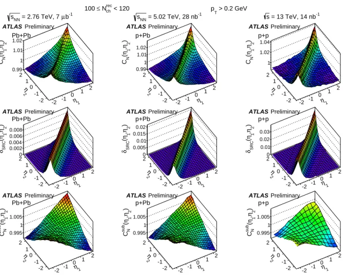
This note presents the measurement of the two-dimensional (2-D) correlation function

C_N

(

η₁, η₂

) over the pseudorapidity range of ∣

η

∣ < 2.4 in √

sNN=

2.76 TeV Pb

+

Pb, √

s_NN=

5.02 TeV

p+

Pb and √

s=

13 TeV

pp

collisions, using the ATLAS detector.

¹

The analysis is performed using events for which the total number of reconstructed charged particles,

N_ch^rec

, with ∣

η

∣ < 2.5 and transverse momentum

p_T

> 0.4 GeV, is in the range 10 ≤

N_ch^rec

< 300. Both the Pb

+

Pb and

p+

Pb data cover this range of

N_ch^rec

, but for

pp

the range extends only to ∼ 150. The measured

C_N

(η

₁, η₂

) is separated into a short-range component

δ_SRC

(η

₁, η₂

) and a long-range component

C^sub_N

(

η1, η2

) . The nature of the FB fluctuation in each collision system is studied by projections of

C^sub_N

(

η₁, η₂

) , as well as from the Legendre coe

ffi

cients ⟨a

_na_m

⟩ obtained from

C^sub_N

(η

₁, η₂

) . The magnitudes of the FB fluctuations are compared for the three systems at similar event multiplicity.

2 ATLAS detector and trigger

The ATLAS detector [17] provides nearly full solid-angle coverage of the collision point with tracking detectors, calorimeters and muon chambers, and is well suited for measurement of two-particle correla- tions over a large pseudorapidity range. The measurements were performed using the inner detector (ID), minimum-bias trigger scintillators (MBTS), the forward calorimeter (FCal), the zero-degree calorimet- ers (ZDC) and the trigger and data acquisition systems. The ID detects charged particles within ∣η∣ < 2.5 using a combination of silicon pixel detectors, silicon micro-strip detectors (SCT), and a straw-tube trans- ition radiation tracker (TRT), all immersed in a 2 T axial magnetic field [18]. An additional pixel layer, the “Insertable B Layer” (IBL) [19,

20] installed between Run 1 and Run 2, is used in the 13 TeV pp

measurements. The MBTS system detects charged particles over 2.1 ≲ ∣η∣ ≲ 3.9 using two hodoscopes of counters positioned at

z

= ± 3.6 m. The FCal consists of three sampling layers, longitudinal in shower depth, and covers 3.2 < ∣

η

∣ < 4.9. The ZDC, available in the Pb

+

Pb and

p+

Pb runs, are positioned at

± 140 m from the collision point, detecting neutrons and photons with ∣η∣ > 8.3.

This analysis uses approximately 7

µb⁻¹

of Pb

+

Pb data, 28 nb

⁻¹

of

p+

Pb data, and 14 nb

⁻¹

of

pp

data taken by the ATLAS experiment at the LHC. The Pb+Pb data were collected in 2010 at a nucleon- nucleon centre-of-mass energy √

s_NN

= 2.76 TeV. The

p+Pb data were collected in 2013, when the LHC

was configured with a 4 TeV proton beam and a 1.57 TeV per-nucleon Pb beam that together produced collisions at √

s_NN

= 5.02 TeV. The higher energy of the proton beam results in a rapidity shift of 0.47 of the nucleon–nucleon center-of-mass frame towards the proton beam direction relative to the ATLAS rest frame. The

pp

data were collected during a low-luminosity operation of the LHC in June 2015 at collision energy √

s

= 13 TeV.

1ATLAS uses a right-handed coordinate system with its origin at the nominal interaction point (IP) in the centre of the detector and thez-axis along the beam pipe. The x-axis points from the IP to the centre of the LHC ring, and they-axis points upward. Cylindrical coordinates(r, φ)are used in the transverse plane,φbeing the azimuthal angle around the beam pipe.

The pseudorapidity is defined in terms of the polar angleθasη= −ln tan(θ/2).

The ATLAS trigger system [21] consists of a Level-1 (L1) trigger implemented using a combination of dedicated electronics and programmable logic, and a high-level trigger (HLT) implemented in processors.

The HLT reconstructs charged-particle tracks using methods similar to those applied in the o

ffl

ine ana- lysis, allowing high-multiplicity triggers (HMT) that select on the number of tracks having

p_T

> 0.4 GeV associated with a single primary vertex. The Pb+Pb data used in the analysis are collected by a minimum- bias trigger, while the

pp

and

p+

Pb data are collected by a minimum-bias trigger and a HMT.

The Pb+Pb trigger requires signals in two ZDCs or either of the two MBTS counters. The ZDC trigger thresholds on each side are set below the peak corresponding to a single neutron. A timing requirement based on signals from each side of the MBTS is imposed to remove beam backgrounds. The minimum- bias trigger for

p+Pb is similar, except that only the ZDC on the Pb-fragmentation side is used. For pp,

the minimum-bias trigger required only one or more signals in the MBTS.

The HMT trigger used for 13 TeV

pp

analysis selected events at L1 that have a signal in at least one counter on each side of the MBTS, and at HLT have at least 900 SCT hits and at least 60 tracks associated to a primary vertex at the HLT. For the

p+

Pb data, the HMT triggers were formed from a combination of L1 triggers that applied di

ff

erent thresholds on total transverse energy measured over 3.2 < ∣

η

∣ < 4.9 and HLT triggers that applied minimum requirements on the number of HLT-reconstructed tracks. Details of the minimum-bias and HMT triggers can be found in Ref. [22,

23] and Ref. [24,25] for thepp

and

p+Pb

collisions, respectively.

3 Data Analysis

3.1 Event and track selection

The offline event selection for the

p+Pb and pp

data requires at least one reconstructed vertex with its

z

position satisfying ∣z

_vtx

∣ < 100 mm. The mean collision rate per crossing,

µ, is around 0.03 for p+

Pb data and varied between 0.002 and 0.04 for the 13 TeV

pp

data. Events containing multiple collisions are suppressed by rejecting events containing more than one good reconstructed vertex. The

p+Pb events

also require a time difference ∣

∆t∣ <

10 ns between signals in the MBTS trigger counters on either side of the interaction point to suppress non-collision backgrounds.

The offline event selection for the Pb+Pb data requires a reconstructed vertex with its

z

position satisfying

∣z

_vtx

∣ < 100 mm. The selection also requires a time di

ff

erence ∣

∆t∣ <

3 ns between signals in the MBTS trigger counters on either side of the interaction point to suppress non-collision backgrounds. A coincid- ence between the ZDC signals at forward and backward pseudorapidity is required to reject a variety of background processes, while maintaining high e

ffi

ciency for inelastic processes.

Charged-particle tracks and primary vertices are reconstructed in the ID using algorithms whose im-

plementation was optimized for better performance between LHC Runs 1 and 2. In order to compare

directly the

p+

Pb and Pb

+

Pb systems using event selections based on the multiplicity of the collisions,

a subset of data from peripheral Pb+Pb collisions, collected during the 2010 LHC heavy-ion run with

a minimum-bias trigger, was reanalyzed using the same track reconstruction algorithm as that used for

p+

Pb collisions. For the

p+

Pb and Pb

+

Pb analyses, tracks are required to have a

p_T

-dependent minimum

number of hits in the SCT, and the transverse (d

0

) and longitudinal (z

0

sin

θ) impact parameters of the

track relative to the vertex are required to be less than 1.5 mm. The tracks are also required to satisfy

∣

d₀

∣/

σd₀

< 3 and ∣

z₀

sin

θ

/

σz

∣ < 3, respectively, where

σd₀

and

σz

are uncertainties on

d₀

and

z₀

sin

θ

ob- tained from the track-fit covariance matrix. A description of the 2010 Pb+Pb data and 2013

p+Pb data

can be found in Ref. [3] and Ref. [26], respectively.

For the 13 TeV

pp

analysis, the selection criteria have been modified slightly to profit from the presence of the IBL in Run 2. Furthermore, the requirements of ∣d

₀^z

∣ < 1.5 mm and ∣z

₀

sin

θ∣ <

1.5 mm are applied, where

d₀^z

is the transverse impact parameter of the track relative to the average beam position. These selection criteria are the same as those in Refs. [22,

23].

In this note, the correlation functions are constructed using tracks passing the above selection cuts and which have

p_T

> 0.2 GeV and ∣

η

∣ < 2.4. However, slightly di

ff

erent kinematic thresholds,

p_T

> 0.4 GeV and ∣η∣ < 2.5, are used to count the number of reconstructed charged particles of the event, denoted by

N_ch^rec

.

The efficiency of the track reconstruction and track selection requirements,

(η,p_T

) , is evaluated using simulated

p+Pb or Pb+Pb events produced with the HIJING event generator [27] or simulatedpp

events from the Pythia 8 [28] event generator using parameter settings according to the so-called A2 tune [29]).

The response of the detector to these Monte Carlo (MC) events is simulated using GEANT4 [30,

31]

and the resulting events are reconstructed with the same algorithms that are applied to the data. The e

ffi

ciencies for the three datasets are similar for events with similar multiplicity. Small di

ff

erences are due to changes in the detector conditions in Run 1 and changes in the reconstruction algorithm between Runs 1 and 2. In the simulated events, the efficiency reduces the measured charged-particle multiplicity relative to the event generator multiplicity for primary charged particles.

²

The reduction factors for

N_ch^rec

and associated e

ffi

ciency uncertainties are

b

= 1.29 ± 0.05, 1.29 ± 0.05 and 1.18 ± 0.05 for Pb

+

Pb,

p+Pb and pp

collisions, respectively. The values of these reduction factors are found to be multiplicity independent over the

N_ch^rec

range used in this analysis, 10 ≤

N_ch^rec

< 300. Therefore, these factors are used to multiply the

N_ch^rec

to obtain the e

ffi

ciency-corrected average number of charged particles with

p_T

> 0.4 GeV and ∣η∣ < 2.5,

N_ch

=

bN^rec_ch

. The quantity

N_ch

is used when presenting the multiplicity dependence of the SRC and the LRC.

3.2 Two-particle correlations

The two-particle correlation function defined in Eq.

1

is constructed as the ratio of distributions for same- event pairs, or foreground pairs

S

(η

₁, η₂

) ∝ ⟨N(η

₁

)N(η

₂

)⟩ , and mixed-event pairs, or background pairs

B(η₁, η₂

) ∝ ⟨N(

η₁

)⟩ ⟨N(

η₂

)⟩ :

C(η₁, η₂

) =

S

(

η₁, η₂

)

B(η₁, η₂

)

.

(12)

The mixed-event pair distribution is constructed by combining tracks from the foreground event with another event with similar

N_ch^rec

(matched within two tracks) and

z_vtx

(matched within 2.5 mm). The events are also required to be close to each other in time to account for possible time-dependent variation of the detector conditions. The mixed-event distribution should account properly for detector ine

ffi

ciencies and non-uniformity, but does not contain physical correlations. The normalization of

C(η₁, η₂

) is chosen such that its average value in the

η₁

,

η₂

plane is one. The correlation function satisfies the symmetry

C(η₁, η₂

) =

C(η₂, η₁

) and, for a symmetric collision system,

C(η₁, η₂

) =

C(−η₁,

−η

₂

) . Therefore, for

pp

and Pb

+

Pb collisions, pairs are filled in one quadrant of the (

η₁, η₂

) space defined by

η−

≡

η₁

−

η₂

> 0

2For Pb+Pb andp+Pb simulation, it includes charged particles which originate directly from the collision or result from decays of particles withcτ<10 mm. The definition for primary charged particles is somewhat stronger inppsimulation [22].

η1

-2 -1 0 1 2

2

η -2 -1 0 1 2 ) 2η, 1η(+- C

0.995 1 1.005 1.01 1.015

ATLAS Preliminary Pb+Pb

η1

-2 -1 0 1 2

2η -2 -1 0 1 2 ) 2η, 1η(±±C

0.995 1 1.005

ATLAS Preliminary Pb+Pb

η1

-2 -1 0 1 2

2η -2 -1 0 1 2 ) 2η, 1ηR(

1 1.002 1.004 1.006 1.008

ATLAS Preliminary Pb+Pb

η+

-2 0 2

Gaussian Width

0 0.2 0.4 0.6 0.8 1

ATLAS Preliminary Pb+Pb

η+

-5 0 5

) +ηf(

1 1.1

ATLAS Preliminary Pb+Pb

ATLAS Preliminary < 220

rec

Nch

≤ 200

b-1

µ = 2.76 TeV, Pb+Pb, 7 sNN

> 0.2 GeV pT

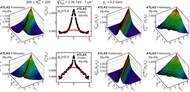
Figure 1: The correlation functions for opposite-charge pairs C⁺⁻(η₁, η₂) (top-left panel), same-charge pairs C^±±(η₁, η₂)(top-middle panel) and the ratioR(η₁, η₂) =C⁺⁻(η₁, η₂)/C^±±(η₁, η₂)(top-right panel) for Pb+Pb col- lisions with 200≤ N_ch^rec<220. The width and magnitude of the short-range peak of the ratio as a function of η+

are shown in the bottom-middle panel and bottom-right panel, respectively. The error bars represent the statistical uncertainties, and the solid lines indicate a quadratic fit. The dotted line in the bottom-right panel serves to better indicate the deviation of f(η+)from 1.

and

η+

≡

η₁

+

η₂

> 0 and then reflected to the other quadrants. For

p+Pb collisions, pairs are filled in one

half of the (

η₁, η₂

) space defined by

η₁

−

η₂

> 0 and then reflected to the other half. To correct

S

(

η₁, η₂

) and

B

(

η₁, η₂

) for the individual ine

ffi

ciencies of particles in the pair, the pairs are weighted by the inverse product of their tracking efficiencies 1 /(

₁₂

) . Remaining detector distortions not accounted for by the reconstruction e

ffi

ciency largely cancel in the same-event to mixed-event ratio.

Figure

1

shows separately the correlation functions for same-charge pairs and opposite-charge pairs from Pb+Pb collisions with 200 ≤

N_ch^rec

< 220. The ratio of the two,

R(η₁, η₂

) =

C⁺⁻

(η

₁, η₂

)/C

^±±

(η

₁, η₂

) , is shown in the top-right panel. The correlation functions show a narrow “ridge”-like shape along

η₁

≈

η₂

(or

η−

≈ 0), and a fall off towards the corners at

η₁

= −η

₂

≈ (or

η+

≈ 0 and

η₁

≈ ± 2.4). The magnitude of the ridge for the opposite-charge pairs is stronger than that for the same-charge pairs, which is characteristic of the influence from SRC from jet fragmentation or resonance decays. In regions away from the SRC, i.e.

large values of ∣η

−

∣ , the ratio approaches unity, suggesting that the magnitude of the LRC is independent

of the charge combinations. To quantify the shape of the SRC in the ratio along

η+

,

R

is expressed in

η1

-2 -1 0 1 2

2

η -2 -1 0 1 2 ) 2η, 1η(+- C

1 1.01 1.02 1.03

ATLAS Preliminary p+Pb

η1

-2 -1 0 1 2

2η -2 -1 0 1 2 ) 2η, 1η(±±C

0.995 1 1.005 1.01 1.015

ATLAS Preliminary p+Pb

η1

-2 -1 0 1 2

2η -2 -1 0 1 2 ) 2η, 1ηR(

1 1.005 1.01 1.015

ATLAS Preliminary p+Pb

η+

-2 0 2

Gaussian Width

0 0.2 0.4 0.6 0.8 1

ATLAS Preliminary p+Pb

η+

-5 0 5

) +ηf(

0.8 1 1.2

1.4 ATLAS Preliminary

p+Pb ATLAS Preliminary

< 220

rec

Nch

≤ 200

= 5.02 TeV, p+Pb, 28 nb-1

sNN

> 0.2 GeV pT

Figure 2: The correlation functions for opposite-charge pairs C⁺⁻(η₁, η₂) (top-left panel), same-charge pairs C^±±(η₁, η₂)(top-middle panel) and the ratioR(η₁, η₂) =C⁺⁻(η₁, η₂)/C^±±(η₁, η₂)(top-right panel) forp+Pb col- lisions with 200≤ N_ch^rec<220. The width and magnitude of the short-range peak of the ratio as a function of η+

are shown in the bottom-middle panel and bottom-right panel, respectively. The error bars represent the statistical uncertainties, and the solid lines indicate a quadratic fit. The dotted line in the bottom-right panel serves to better indicate the deviation of f(η+)from 1.

terms of

η+

and

η−

,

R(η+, η−

) , and the following quantity is calculated:

f

(η

+

) = ∫

0.4

−0.4R(η+, η−

)/ 0.8

dη−

− 1

∫

−0.40.4 R(

0, η

−

)/ 0.8

dη−

− 1

.

(13) As shown in Fig.

1, the quantity f

(η

+

) is nearly a constant in Pb+Pb collisions, implying that the SRC is independent of

η+

. To quantify the shape of the SRC along the

η−

direction,

R(η+, η−

) is fit to a gaussian function in slices of

η+

. The width, as shown in the bottom-middle panel of Fig.

1, is constant, suggesting

that the shape of the SRC in

η−

is the same for different

η+

slices.

Figure

2

shows the correlation function in

p+

Pb collisions with similar multiplicity to the Pb

+

Pb data in

Fig.

1. The correlation function shows a significant asymmetry between the proton-going side (positive η+

) and lead-going side (negative

η+

). However, much of this asymmetry appears to be confined to a

small ∣

η−

∣ region where the SRC dominates. The magnitude of the SRC, estimated by

f

(

η+

) shown in

the bottom-right panel, increases by about 40% from the lead-going side (negative

η+

) to the proton-

going side (positive

η+

), but the width of SRC in

η−

is independent of

η+

as shown in the bottom-middle

panel. In contrast, the LRC correlation has no dependence on the charge combinations, as the value of

R

approaches unity at large ∣

η−

∣ .

As discussed in the introduction, the shape of the single-particle multiplicity distribution and track re- construction efficiency may vary with event centrality, and therefore the distribution of ⟨N(η)⟩ could also vary with event activity. This residual single-particle mode cancels in the ratio

R(η₁, η₂

) , but could dis- tort the correlation function

C

(

η₁, η₂

) . The single-particle mode is removed using Eq.

2, as discussed

further in the introduction. The resulting distribution

C_N

(η

₁, η₂

) is then separated into SRC and LRC components using the procedure discussed in the next section.

3.3 Separation of the short-range correlation and the long-range correlation

In order to quantify the features of the correlation function, it is essential to develop a method to estimate and separate the contributions from the SRC and the LRC. The ratio

R(η₁, η₂

) serves as a valuable tool for this estimation, as it is insensitive to the LRC and single particle modes.

Expressing

η₁

and

η₂

in terms of

η+

and

η−

, the ratio of the correlation function between opposite-charge and same-charge pairs can be approximated by:

R(η+, η−

) ≈ 1 +

δ⁺⁻_SRC

(η

+, η−

) −

δ^±±_SRC

(η

+, η−

) (14) where the two

δ⁺⁻_SRC

and

δ^±±_SRC

distributions represent the SRC for the opposite-charge pairs and same- charge pairs, respectively, and the LRC and single-particle modes cancel out in the ratio, since all relevant deviations from 1 are small. Assuming that the shape of the SRC component factorizes in

η−

and

η+

, and that the shape along the

η+

is the same for the opposite-charge and same-charge pairs, then

R(η+, η−

) can be further simplified as:

R(η+, η−

) ≈ 1 +

f

(η

+

) [g

⁺⁻

(η

−

) −

g^±±

(η

−

)]

, δ⁺⁻_SRC

=

f

(η

+

)g

⁺⁻

(η

−

), δ

^±±_SRC

=

f

(η

+

)g

^±±

(η

−

) (15) where

f

(

η+

) describes the shape along

η+

and can be calculated via Eq.

13. The functionsg⁺⁻

and

g^±±

describe the SRC along the

η−

direction for the two charge combinations, which differ in both magnitude and shape.

In order to estimate the

g(η−

) functions, the

C_N

(η

+, η−

) distributions are projected into 1-D

η−

distri- butions over a narrow slice ∣η

+

∣ < 0.4. The distributions, denoted by

C_N

(η

−

) , are shown in the second column of Fig.

3

for the opposite-charge and the same-charge pairs separately for Pb

+

Pb collisions. The SRC appears as a narrow peak on top of a distribution that has an approximately quadratic shape. There- fore a quadratic fit is applied to the data in the region of ∣η

−

∣ > 1.5, and the difference between the data and fit in the ∣

η−

∣ < 2 region is taken as the estimated SRC component or the

g

(

η−

) function, which is assumed to be zero for ∣η

−

∣ > 2. This range ( ∣η

−

∣ > 1.5) is about twice the width of the short-range peak in the

R(η+, η−

) distribution along the

η−

direction (examples are given in the bottom-middle panel of Figs.

1

and

2). This width is observed to decrease from 0.9 to 0.7 as a function ofN_ch^rec

in the

p+

Pb collisions, and is slightly broader in Pb

+

Pb collisions and slightly narrower in

pp

collisions at the same

N_ch^rec

. The range of the fit is varied from ∣η

−

∣ > 1.5 to ∣η

−

∣ > 2.0 to check the sensitivity of the SRC estimation, and the variation is included in the final systematic uncertainties. Furthermore, this study is also repeated for

CN

(

η−

) obtained in several other

η+

slices within ∣

η+

∣ < 1.2, and consistent results are obtained.

Once the distribution

g(η−

) is obtained from the fit, it is multiplied by the

f

(η

+

) function calculated from

the

R(η+, η−

) using Eq.

13, to obtain theδ_SRC

(

η₁, η₂

) (Eq.

15) in the full phase space. The procedure is

repeated separately for all-charge, opposite-charge and same-charge pairs. The estimated correlation is

shown in the third column of Fig.

3. Subtracting this distribution from theC_N

(η

₁, η₂

) and then removing

η1

-2 -1 0 1 2

2η -2 -1 0 1 2 ) 2η, 1η(+- NC _0.995¹

1.005 1.01 1.015

ATLASPreliminary Pb+Pb

η-

-5 0 5

+-) -η(CN

0.995 1

1.005 |η₊|<0.4 ^ATLAS_Prelim.

Pb+Pb

η1

-2 -1 0 1 2

2η -2 -1 0 1 2 ) 2η, 1η(+- SRCδ ⁰

0.005 0.01

ATLASPreliminary Pb+Pb

η1

-2 -1 0 1 2

2η -2 -1 0 1 2 ) 2η, 1η(sub,+- NC

1 1.005

ATLASPreliminary Pb+Pb

η1

-2 -1 0 1 2

2η -2 -1 0 1 2 ) 2η, 1η(±± NC

0.995 1 1.005

ATLASPreliminary Pb+Pb

η-

-5 0 5

±±) -η(CN

0.996 0.998 1

1.002 |η₊|<0.4 ^ATLAS_Prelim.

Pb+Pb

η1

-2 -1 0 1 2

2η -2 -1 0 1 2 ) 2η, 1η(±± SRCδ ^00.001

0.002 0.003

ATLASPreliminary Pb+Pb

η1

-2 -1 0 1 2

2η -2 -1 0 1 2 ) 2η, 1η(±±sub, NC

1 1.005

ATLASPreliminary Pb+Pb < 220

rec

Nch

≤

200 s_NN = 2.76 TeV, 7 µb^-1 > 0.2 GeV

pT

Figure 3: The separation of correlation functions (first column) into the SRC (third column) and LRC (last column) for Pb+Pb collisions with 200 ≤ N_ch^rec <220, separately for the opposite-charge pairs (top row) and same-charge pairs (bottom row). The second column shows the quadratic fit in ∣η−∣ > 1.5 of the 1-D correlation function projected over the∣η+∣ < 0.4 slice, which is used to estimate the SRC component. The error bars represent the statistical uncertainties.

η1

-2 -1 0 1 2

2η -2 -1 0 1 2 ) 2η, 1η(+- NC ¹

1.01 1.02

ATLASPreliminary p+Pb

η-

-5 0 5

+-) -η(CN

0.995 1 1.005

1.01|η₊|<0.4 ^ATLAS_Prelim.

p+Pb

η1

-2 -1 0 1 2

2η -2 -1 0 1 2 ) 2η, 1η(+- SRCδ 0

0.01 0.02

ATLASPreliminary p+Pb

η1

-2 -1 0 1 2

2η -2 -1 0 1 2 ) 2η, 1η(sub,+- NC

1 1.005

ATLASPreliminary p+Pb

η1

-2 -1 0 1 2

2η -2 -1 0 1 2 ) 2η, 1η(±± NC _0.995¹

1.005 1.01 1.015

ATLASPreliminary p+Pb

η-

-5 0 5

±±) -η(CN

0.995 1

1.005 |η₊|<0.4 ^ATLAS_Prelim.

p+Pb

η1

-2 -1 0 1 2

2η -2 -1 0 1 2 ) 2η, 1η(±± SRCδ 0 0.005 0.01

ATLASPreliminary p+Pb

η1

-2 -1 0 1 2

2η -2 -1 0 1 2 ) 2η, 1η(±±sub, NC

1 1.005

ATLASPreliminary p+Pb

< 220

rec

Nch

≤

200 s_NN = 5.02 TeV, 28 nb^-1 > 0.2 GeV

pT

Figure 4: The separation of correlation functions (first column) into the SRC (third column) and LRC (last column) forp+Pb collisions with 200≤N^rec_ch <220, separately for the opposite-charge pairs (top row) and same-charge pairs (bottom row). The second column shows the quadratic fit in∣η−∣ >1.5 of the 1-D correlation function projected over the∣η+∣ < 0.4 slice, which is used to estimate the SRC component. The error bars represent the statistical uncertainties.

a residual small single-particle mode via the normalization procedure of Eq.

2, one obtains the estimated

correlation function containing only the LRC component. This distribution, denoted by

C^sub_N

(η

₁, η₂

) , is shown in the last column of Fig.

3. Despite the fact that the estimated SRC component for the opposite-

charge pairs is more than a factor of two larger than that for the same-charge pairs, the final correlation functions

C^sub_N

(η

₁, η₂

) are very similar. This indicates that the subtraction procedure is quite robust in separating the SRC from the LRC, and the level of agreement between the two charge combinations can be used to estimate the systematic uncertainty associated with the subtraction procedure.

Figure

4

shows similar results from the

p+Pb collisions, and the basic features are the same. It can

be seen that the asymmetry between +

η+

and −

η+

along the diagonal direction comes mainly from the SRC component. The subtracted correlation functions

C_N^sub

(η

₁, η₂

) have very little asymmetry and are consistent between the two charge combinations.

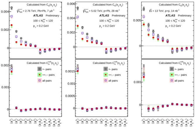
3.4 Quantifying the magnitude of the forward-backward multiplicity fluctuations

In the azimuthal correlation analysis, the azimuthal structure of the correlation function is characterized by harmonic coefficients

vn

obtained via a Fourier decomposition [3,

32]. A similar approach can be

applied for pseudorapidity correlations [9,

15]. Following Eq.5, the correlation functions are expanded

into Legendre polynomial functions, and the two-particle Legendre coe

ffi

cients ⟨a

_na_m

⟩ are calculated directly from the correlation function according to Eq.

7. The two-particle correlation method measures,

in effect, the RMS values of the EbyE

a_n

, and the final results on the coefficients are presented in terms of

√

∣ ⟨a

_na_m

⟩ ∣ . As a consequence of the condition for a symmetric collision system, the odd and even coefficients should be uncorrelated in

pp

and Pb+Pb collisions:

a_n,n+1

= ⟨a

_na_n+1

⟩ = 0

.

(16)

However, even in

p+

Pb collisions, the correlation function after SRC removal,

C_N^sub

(

η₁, η₂

) , is observed to be nearly symmetric between

η

and −η (right column of Fig.

4), and hence

⟨a

na_n+1

⟩ values are very small and ignored in this note.

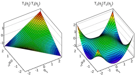
The shape of the first two Legendre bases in 2-D are shown in Fig.

5. The first base function has the

shape of

η₁η₂

and is directly sensitive to the FB asymmetry of the EbyE fluctuation. The second base has a quadratic shape in the

η₁

and

η₂

directions and is sensitive to the EbyE fluctuation in the width of the

N(η)

distribution. It will be seen in Sec.

4

that the data require only the first term, in which case the shape of the correlation function can be approximated by:

C^sub_N

(η

₁, η₂

) ≈ 1 + ⟨a

²₁

⟩

η₁η₂

= 1 +

⟨

a²₁

⟩

4 (η

²₊

−

η²₋

)

.

(17)

Therefore a quadratic shape is expected along the two diagonal directions,

η+

and

η−

, of the correlation function, and the

√

⟨

a²₁

⟩ coefficient can be calculated by a simple quadratic fit of

C^sub_N

in narrow slices of

η−

or

η+

.

Alternatively,

√

⟨

a²₁

⟩ can also be estimated from a simple ratio:

r_N^sub

(η, η

_ref

) = {

C^sub_N

(−

η, η_ref

)/C

^sub_N

(

η, η_ref

)

, η_ref

> 0

C^sub_N

(η, −η

_ref

)/C

^sub_N

(−η, −η

_ref

)

, η_ref

< 0 (18)

≈ 1 − 2 ⟨a

²₁

⟩

ηη_ref,

(19)

η1

-2

-1 0 1 2

2η -2 -1 0 1 2 -1 0 1

1) η

1(

T )

η2 1( T

η1

-2

-1 0 1 2

2

η -2 -1 0 1 2 -1 0 1 2

1) η

2(

T )

η2 2( T

Figure 5: The shape of the first two Legendre base functions associated witha_1,1 anda_2,2 in the two-particle correlation function.

where

η_ref

is a narrow pseudorapidity interval. This correlator has the advantage that most of the single- particle modes are even functions in

η, so they cancel in the ratios. Therefore, this correlator provides

a robust consistency check of any potential bias induced by the renormalization procedure of Eq.

2. A

similar quantity can be calculated also for

C_N

(η

₁, η₂

) , denoted by

r_N

(η, η

_ref

) .

In summary, this note uses the following four di

ff

erent methods to estimate

√

⟨a

²₁

⟩ : 1. Legendre decomposition of the 2-D correlation function

C^sub_N

(η

+, η−

) , via Eq.

5.

2. Quadratic fit of

C^sub_N

(η

−

) in a narrow slice of

η+

, which gives

√

⟨a

²₁

⟩ as a function of

η+

. 3. Quadratic fit of

C^sub_N

(η

+

) in a narrow slice of

η−

, this gives

√

⟨

a²₁

⟩ as a function of

η−

. 4. Linear fit of

r_N^sub

(

η

) in a narrow slice of

η_ref

, this gives

√

⟨a

²₁

⟩ as a function of

η_ref

.

The three fitting methods (2,3,4) use the correlation function in limited and largely non-overlapping re- gions of the

η₁

and

η₂

phase space, and therefore are independent of each other and largely independent of the Legendre decomposition method. However, if the correlation function is dominated by the ⟨

a²₁

⟩ term, the results from all four methods should be consistent.

3.5 Systematic uncertainties

The systematic uncertainties in this analysis arise from the event-mixing, track reconstruction and se- lection efficiency, pair acceptance, and using simulated events to test the analysis process by comparing results from the generated charged particles with those from reconstructed tracks. These uncertainties apply to

C_N

(

η₁, η₂

) or

C^sub_N

(

η₁, η₂

) and the associated Legendre coe

ffi

cients. However, the systematic uncertainty on

C^sub_N

(η

₁, η₂

) also depends on the procedure for separating the SRC from the LRC.

A natural way of quantifying these systematic uncertainties is to calculate

C_N

(

η₁, η₂

) or

C^sub_N

(

η₁, η₂

)

under a di

ff

erent condition, and then construct the ratio to the default analysis:

d

(

η₁, η₂

) . The average