ATLAS NOTE ATLAS-CONF-2015-043

A TLAS-CONF-2015-043 31/08/2015

ATLAS NOTE

ATLAS-CONF-2015-043

31st August 2015

Search for evidence for strong gravity in jet final states produced in pp collisions at √

s = 13 TeV using the ATLAS detector at the LHC

The ATLAS Collaboration

Abstract

A search is conducted for new physics in multijet final states using data from proton-proton collisions at √

s = 13 TeV taken at the CERN LHC with the ATLAS detector. Events are selected containing at least three jets with scalar sum of transverse momentum (H

) greater than 1 TeV. No excess is seen at large H

and limits are presented in terms of new physics models that hypothesize additional space-time dimensions.

© 2015 CERN for the benefit of the ATLAS Collaboration.

Reproduction of this article or parts of it is allowed as specified in the CC-BY-3.0 license.

1 Introduction

Most models of low-scale gravity allow the production of non-perturbative gravitational states, such as micro black holes and string balls (highly excited string states) at Large Hadron Collider (LHC) collision energies [1–4]. This is due to the fundamental gravitational scale being comparable to the electroweak scale in these gravity models. If black holes or string balls with masses much higher than this funda- mental gravitational scale are produced at the LHC, they behave as classical thermal states and decay to a relatively large number of high transverse momentum (p

) particles. One of the predictions of these models is the expectation that particles are emitted from black holes at relative rates which primarily depend on the number of Standard Model (SM) degrees of freedom (number of charge, spin, flavour, and colour states). Spin dependent e ff ects, such as the Fermi-Dirac and Bose-Einstein distributions in statistical mechanics, and gravitational transmission factors (also dependent on spin) are less important.

Several searches were carried out using data from Run-1 at the LHC at centre-of-mass energies of 7 and 8 TeV by ATLAS [5–9] and CMS [10–12]. The analysis described here follows the method of a similar ATLAS result from 8 TeV data [5]. The increase in the LHC energy to 13 TeV in Run-2 brings a large increase in the sensitivity compared to Run-1.

Identification of high-p

, high-multiplicity final states resulting from the decay of high-mass objects is accomplished by studying the scalar sum of the jet p

(H

). A low-H

control region is defined. New physics is not expected to contribute in this region owing to the exclusion limits set by the previous searches mentioned above. A fit-based technique is used to extrapolate from the control region to a high-H

signal region to estimate the amount of the SM background. The observation is compared to the background-only expectation determined by the fit-based method. In the absence of significant deviations from the background-only expectation, a 95% Confidence Level (CL) limit on the black hole production is set. The limit is given in terms of parameters used in the CHARYBDIS2 1.0.4 [13] model, specifically on the number of extra dimensions (n) and the threshold for production.

The production and decay of black holes and string balls lead to final states distinguished by a high multi- plicity of high-p

particles, consisting mostly of jets arising from quark and gluon emission. Since black hole decays are considered to be a stochastic process, di ff erent numbers of particles, and consequently jets, are emitted from black holes with identical kinematic distributions. This motivates the search in inclusive jet multiplicity slices, rather than optimizing a potential signal-to-background for a particular exclusive jet multiplicity.

The analysis is not optimized for any particular model. However, for the purpose of comparison to other searches both within ATLAS and between the LHC experiments, CHARYBDIS2 1.0.4 is used with the number of extra dimensions in the model fixed to six and the black hole required to be rotating.

2 ATLAS detector

The ATLAS detector [14] covers almost the whole solid angle around the collision point with layers of tracking detectors, calorimeters and muon chambers. For the measurements presented in this note, the calorimeters are of particular importance. The inner detector, immersed in a magnetic field provided by a solenoid, has full coverage in φ and covers the pseudorapidity range |η | < 2.5 1. It consists of

1

ATLAS uses a right-handed coordinate system with its origin at the nominal interaction point in the centre of the detector

and the z-axis along the beam direction. The x-axis points toward the centre of the LHC ring, and the y-axis points upward.

a silicon pixel detector, a silicon microstrip detector and a transition radiation straw-tube tracker. The innermost pixel layer, the insertable B-layer, was added between Run-1 and Run-2 of the LHC, around a new thinner (radius of 25 mm) beam pipe. In the pseudorapidity region |η | < 3.2, high granularity liquid- argon (LAr) electromagnetic (EM) sampling calorimeters are used. An iron-scintillator tile calorimeter provides hadronic coverage over |η | < 1.7. The end-cap and forward regions, spanning 1.5 < |η| < 4.9, are instrumented with LAr calorimetry for both EM and hadronic measurements. The muon spectrometer surrounds these, and comprises a system of precision tracking chambers and trigger detectors with three large toroids, each consisting of eight coils providing magnetic field for the muon detectors.

The ATLAS detector has a two-level trigger system: the level-1 hardware stage and the high-level trigger software stage. The events used in this search are selected using a high-H

trigger, which requires at least one jet of hadrons with p

> 200 GeV, and a high scalar sum of transverse momentum of all the jets in the events, H

> 0.85 TeV. In this analysis, a requirement of H

> 1 TeV is applied, for which the trigger is fully e ffi cient. All jets included in the computation of H

are required to satisfy p

> 50 GeV and |η | < 2.8.

3 Event selection

The data used here were recorded in August 2015, with the LHC operating at a centre-of-mass energy of √

s = 13 TeV. The dataset does not include earlier data due to an ine ffi ciency in the triggering of very high energy objects. All detector elements are required to be fully operational, and a total integrated luminosity of 80 pb

is used in this analysis with an uncertainty of 9%. It is derived following the same methodology as that detailed in Ref. [15], from a preliminary calibration of the luminosity scale using a pair of x-y beam-separation scans performed in June 2015.

Events are required to have a primary vertex with at least two associated tracks with p

above 400 MeV.

The primary vertex assigned to the hard scattering collision is the one with the highest P

track

p

, where the scalar sum of track p

is taken over all tracks associated with that vertex.

Since black holes and string balls are expected to decay predominantly to quarks and gluons, the search is simplified by considering only jets. The analysis uses jets of hadrons, as well as misidentified jets arising from photons, electrons, and taus. The calibration of photons, electrons, and taus using the hadronic energy calibration leads to small energy shifts for these objects. Since a particle of this type is expected to occur in less than 0.6% (as determined from simulation studies) of the events in the data sample, they do not contribute significantly to the resolution of H

.

The anti-k

algorithm [16] is used for jet finding, with a distance parameter R = 0.4. The inputs to the jet reconstruction are three-dimensional topo-clusters [17]. This method first clusters together topologi- cally connected calorimeter cells and then classifies these clusters as either electromagnetic or hadronic.

These four-momenta are calibrated for the response to incident hadrons using the procedures described in Refs. [18, 19]. The agreement between data and simulation is further improved by the application of calibration constants obtained at lower collision energies with in situ techniques [20] and validated for use at 13 TeV [21].

Cylindrical coordinates (r, φ) are used in the transverse plane, φ being the azimuthal angle around the beam pipe. The

pseudorapidity η is defined in terms of the polar angle θ by η ≡ − ln[tan(θ/2)].

While a data driven method is used to estimate the background, simulated samples are used to establish, test and validate the methodology of the analysis. Therefore simulation is not required to accurately de- scribe the background, but it should be su ffi ciently similar that the strategy can be tested before applying it to data. Multijet events constitute the dominant background in the search region, with small contribu- tions from t¯ t and γ + jets; W + jets, Z + jets, single-top quark, and diboson background contributions are negligible.

The baseline multijet sample of inclusive jets was generated using PYTHIA 8.1605 [22] implementing leading order (LO) perturbative QCD matrix elements with NNPDF23_ lo_ as_ 0130_ qed parton dis- tribution function (PDF)’s [23] for 2 → 2 processes and p

-ordered parton showers calculated in a leading-logarithmic approximation with the ATLAS A14 tune [24] and the CT10 [25] PDFs. A rea- sonable agreement in the shape of the H

distribution was observed in Run-1 for different inclusive jet multiplicity categories [5]. All Monte-Carlo (MC) simulated background samples are passed through a full GEANT4 [26] simulation of the ATLAS detector [27]. Signal samples are generated from the CHARYBDIS2 1.0.4 [13] MC event generator, which is run with leading-order PDF CTEQ6L1 [28] and uses the PYTHIA 8.160 generator for fragmentation with the ATLAS A14 tune [24]. The most important parameters that have significant e ff ects on black hole production are the e ff ective Planck scale M

in the (4+n)-dimensional world and the black hole mass threshold M

. Signal samples are generated on a grid of M

and M

. The signal samples are passed through a fast detector simulation AtlFast-II [29]. All simulated signal and background samples are reconstructed using the same software as the data.

4 Analysis Strategy

The search is performed by examining the H

distribution for several inclusive jet multiplicities. For each multiplicity, three regions of H

are used: control (C < H

< V ), validation (V < H

< S) and signal (H

> S). Data in the control region are fitted to an empirical function which is then extrapolated to predict the event rate in the validation and signal regions in the absence of new physics. The boundaries of these regions (C, V and S) depend on the integrated luminosity of the data sample used and inclusive jet multiplicity requirement. The following criteria must be satisfied. The lower boundary of the control region (C) should be sufficiently large that the shape of the H

distribution near the boundary is not distorted by trigger or event selection effects. Contamination of possible signal from new physics in the control region must be small for all possible signals not excluded by prior results. There should be some background events in the validation region, with a small signal to background ratio from signals that are not excluded by a previous analysis, so that the background extrapolation can be checked. The signal region is defined so that the background extrapolation uncertainty relative to the background prediction is small2.

A large increase in sensitivity to new physics is expected in Run-2 due primarily to the increase in centre- of-mass energy. A data set of order of a few tens of pb

has such a large range of sensitivity that significant signal contamination in the control and validation region is possible in a data set of this size.

Therefore a bootstrap approach is adopted and data sets are examined whose size increases by approxi- mately a factor of ten at each step, starting with a sample whose sensitivity is slightly beyond the Run-1 limit; simulation studies indicate an initial integrated luminosity of 5 pb

is sufficient for this first step.

This will ensure that if a search in one step sees no new physics, the possible contributions of signal to the

2

The signal region boundary S is chosen so that the (PE-based, see below) background extrapolation uncertainty is less than

0.5 events for H

≥ S.

control and validation regions of the next step are small. For each data set the boundaries of the regions are determined as follows. Simulation is normalized to data in the control region. Since the event rate falls rapidly with H

, this normalization is insensitive to the upper boundary V of the control region. First the lower boundary of the signal region, S, is chosen from this normalized MC so that one background event is expected for H

> S. V is then chosen from this normalized MC so that 20 events are expected for H

> V. This will allow a quantitative comparison of the data and expectation in the validation region to check the extrapolation procedure is working properly.

The total data set used corresponds to an integrated luminosity of 80 pb

and a two step bootstrap is therefore adopted, with 6.5 pb

used in the first step and the remaining 74 pb

used in the second step.

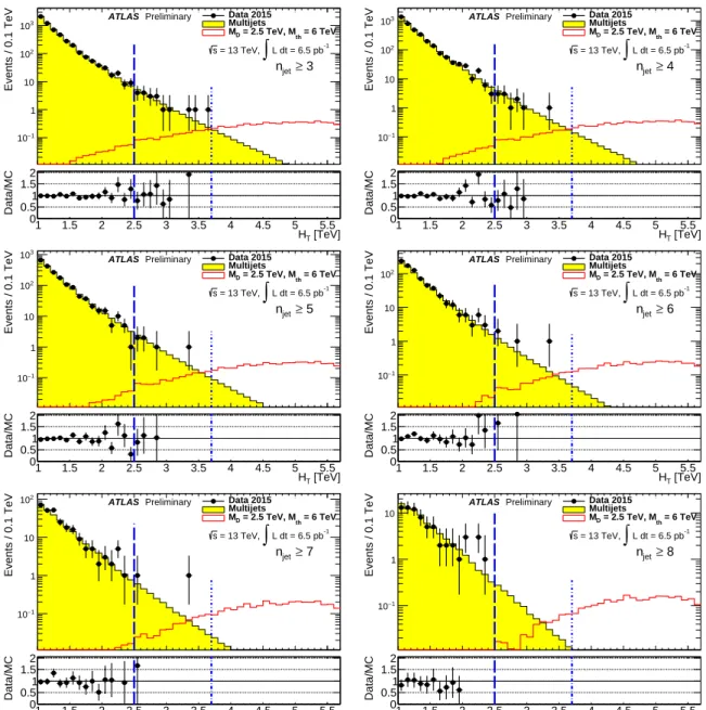
The observed H

distribution is shown in Figure 1 for 6.5 pb

. A comparison is made with MC for illustration. The MC has been normalized to the data in the control region independently in each n

sample. The example signal (M

= 2.5 TeV, M

= 6.0 TeV) shown is just beyond the limit obtained from the 8 TeV analysis. Any possible signal must therefore be smaller than this. Lines delimiting the control, validation and signal regions are shown. The H

distribution expected from this signal is such that any contamination in the control and validation regions is negligible. In addition the contamination in the control region is negligible for all signals that this data set (6.5 pb

) is sensitive to. Possible contamination in the validation region is less than 10% for signals not excluded by the Run-1 analysis.

Therefore it is to be expected that the predicted event rate in the validation regions from fits to the control region should provide a test of the extrapolation procedure. It can be seen from Figure 1 that data sets with high jet multiplicity contain rather few events. This first step analysis therefore uses only jet multiplicity, n

≥ 3.

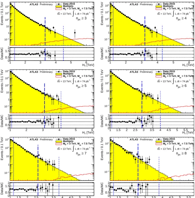
The observed H

distribution from the 74 pb

sample used in the second step is shown in Figure 2 where comparison is made with MC for illustration. The MC has been normalized to the data in the control region independently in each n

sample. Before normalization the ratio Data / MC increases with jet multiplicity from 0.74 to 0.88. This variation is not unexpected since the MC is leading order in QCD.

Signal samples (M

= 3 TeV, M

= 7.5 TeV) are superimposed on data in Figure 2 which correspond approximately to those just beyond the sensitity of the first step analysis. The logic of the previous paragraph applied here shows that the bootstrap approach is protected against signal contamination if data sets increasing by a factor of ten in integrated luminosity are used.

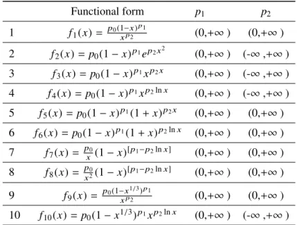
As already mentioned, in order to estimate the number of background events in the validation and signal regions, a data driven method is used. Data in the control region are fitted to an empirical function which is then used to extrapolate to higher H

. The analytic functions considered for this analysis and the allowed ranges of parameters in the fit are summarized in Table 1. Function 1 is the baseline function used to fit background for the Run-1 result [5]. Functions 2 - 10 are the alternative background functions considered or motivated by the Run-1 analysis.

A baseline function is selected and alternate functions are used to estimate the systematic uncertainties on

the predicted backgrounds. Pseudo-experiments (PEs) drawn from samples of the simulated background

are used to evaluate the functions and to assess their ability to obtain a good fit and to correctly predict

the event rates in the validation and signal regions. Fits are required to have good χ

in the control region

and decrease monotonically with H

. Provided these criteria are met, functions are ranked based on the

goodness of their extrapolation in the signal region. The top ranked function is selected as the baseline

function. Any function which satisfies these criteria but whose extrapolation does not agree with the data

in the validation region within 95% confidence level is rejected and its result is not used to obtain the

signal region background prediction.

Events / 0.1 TeV

−1

10 1 10 102

103

ATLAS Preliminary

L dt = 6.5 pb-1

∫

= 13 TeV, s

≥ 3 njet Data 2015 Multijets

= 6 TeV = 2.5 TeV, Mth

MD

[TeV]

HT

1 1.5 2 2.5 3 3.5 4 4.5 5 5.5

Data/MC

0 0.51 1.52

Events / 0.1 TeV

−1

10 1 10 102

103 ATLAS Preliminary

L dt = 6.5 pb-1

∫

= 13 TeV, s

≥ 4 njet Data 2015 Multijets

= 6 TeV = 2.5 TeV, Mth

MD

[TeV]

HT

1 1.5 2 2.5 3 3.5 4 4.5 5 5.5

Data/MC

0 0.51 1.52

Events / 0.1 TeV

−1

10 1 10 102

103 ATLAS Preliminary

L dt = 6.5 pb-1

∫

= 13 TeV, s

≥ 5 njet Data 2015 Multijets

= 6 TeV = 2.5 TeV, Mth

MD

[TeV]

HT

1 1.5 2 2.5 3 3.5 4 4.5 5 5.5

Data/MC

0 0.51 1.52

Events / 0.1 TeV

−1

10 1 10 102

ATLAS Preliminary

L dt = 6.5 pb-1

∫

= 13 TeV, s

≥ 6 njet Data 2015 Multijets

= 6 TeV = 2.5 TeV, Mth

MD

[TeV]

HT

1 1.5 2 2.5 3 3.5 4 4.5 5 5.5

Data/MC

0 0.51 1.52

Events / 0.1 TeV

−1

10 1 10

102 ATLAS Preliminary

L dt = 6.5 pb-1

∫

= 13 TeV, s

≥ 7 njet Data 2015 Multijets

= 6 TeV = 2.5 TeV, Mth

MD

[TeV]

HT

1 1.5 2 2.5 3 3.5 4 4.5 5 5.5

Data/MC

0 0.51 1.52

Events / 0.1 TeV

−1

10 1 10

ATLAS Preliminary

L dt = 6.5 pb-1

∫

= 13 TeV, s

≥ 8 njet Data 2015 Multijets

= 6 TeV = 2.5 TeV, Mth

MD

[TeV]

HT

1 1.5 2 2.5 3 3.5 4 4.5 5 5.5

Data/MC

0 0.51 1.52

Figure 1: Data and MC comparison for H

distributions in di ff erent inclusive n

bins for 6.5 pb

data. The black

hole signal with M

= 2.5 TeV, M

= 6.0 TeV is superimposed with the data and background MC sample. The MC

has been normalized to data in the control region. The vertical dashed line marks the boundary between control

region and validation region, and the dashed-dot line marks the boundary between validation region and signal

region. The values shown correspond to those determined for the n

≥ 3 case. For n

≥ 4, there is insu ffi cient

data in this data set for the analysis to be completed there.

Events / 0.1 TeV

−1

10 1 10 102

103

104 ATLAS Preliminary

L dt = 74 pb-1

∫

= 13 TeV, s

≥ 3 njet Data 2015 Multijets

= 7.5 TeV = 3 TeV, Mth

MD

[TeV]

HT

1 2 3 4 5 6

Data/MC

0 0.51 1.52

Events / 0.1 TeV

−1

10 1 10 102

103

104 ATLAS Preliminary

L dt = 74 pb-1

∫

= 13 TeV, s

≥ 4 njet Data 2015 Multijets

= 7.5 TeV = 3 TeV, Mth

MD

[TeV]

HT

1 2 3 4 5 6

Data/MC

0 0.51 1.52

Events / 0.1 TeV

−1

10 1 10 102

103

104 ATLAS Preliminary

L dt = 74 pb-1

∫

= 13 TeV, s

≥ 5 njet Data 2015 Multijets

= 7.5 TeV = 3 TeV, Mth

MD

[TeV]

HT

1 2 3 4 5 6

Data/MC

0 0.51 1.52

Events / 0.1 TeV

−1

10 1 10 102

103

ATLAS Preliminary

L dt = 74 pb-1

∫

= 13 TeV, s

≥ 6 njet Data 2015 Multijets

= 7.5 TeV = 3 TeV, Mth

MD

[TeV]

HT

1 1.5 2 2.5 3 3.5 4 4.5 5 5.5 6

Data/MC

0 0.51 1.52

Events / 0.1 TeV

−1

10 1 10 102

103 ATLAS Preliminary

L dt = 74 pb-1

∫

= 13 TeV, s

≥ 7 njet Data 2015 Multijets

= 7.5 TeV = 3 TeV, Mth

MD

[TeV]

HT

1 1.5 2 2.5 3 3.5 4 4.5 5 5.5

Data/MC

0 0.51 1.52

Events / 0.1 TeV

−1

10 1 10 102

ATLAS Preliminary

L dt = 74 pb-1

∫

= 13 TeV, s

≥ 8 njet Data 2015 Multijets

= 7.5 TeV = 3 TeV, Mth

MD

[TeV]

HT

1 1.5 2 2.5 3 3.5 4 4.5 5 5.5

Data/MC

0 0.51 1.52

Figure 2: Data and MC comparison for H

distributions in di ff erent inclusive n

bins for the 74 pb

data data sample. The black hole signal with M

= 3 TeV, M

= 7.5 TeV is superimposed with the data and background MC.

The MC has been normalized to data in the control region. The vertical dotted line marks the lower boundary of

the control region, the vertical dashed line marks the boundary between control region and validation region, and

the vertical dashed-dot line marks the boundary between validation region and signal region. These boundaries are

determined for each n

sample separately.

Functional form p

p

1 f

( x) =

(0,+ ∞ ) (0,+ ∞ ) 2 f

(x ) = p

(1 − x)

e

(0,+ ∞ ) (- ∞ ,+ ∞ ) 3 f

(x ) = p

(1 − x)

x

(0, + ∞ ) (-∞ , + ∞ ) 4 f

( x) = p

(1 − x )

x

(0,+ ∞ ) (- ∞ ,+ ∞ ) 5 f

( x) = p

(1 − x )

(1 + x )

(0, + ∞ ) (0, + ∞ ) 6 f

(x ) = p

(1 − x)

(1 + x)

(0,+ ∞ ) (0,+ ∞ ) 7 f

( x) =

(1 − x)

(0, + ∞ ) (0, + ∞ ) 8 f

( x) =

(1 − x)

(0,+ ∞ ) (0,+ ∞ ) 9 f

(x ) =

(0, + ∞ ) (0, + ∞ ) 10 f

(x ) = p

(1 − x

)

x

(0,+ ∞ ) (-∞ ,+ ∞ ) Table 1: Analytic functions considered in this analysis where x = H

/ √

s. p

is a normalization constant. p

and p

are free parameters in a fit, and their allowed floating ranges are shown in the last two columns.

The procedure of ranking and selecting background functions as well as the procedure of determining the control, validation, and signal region boundaries are repeated for the two steps used in the bootstrap process and for analyses with different n

requirements.

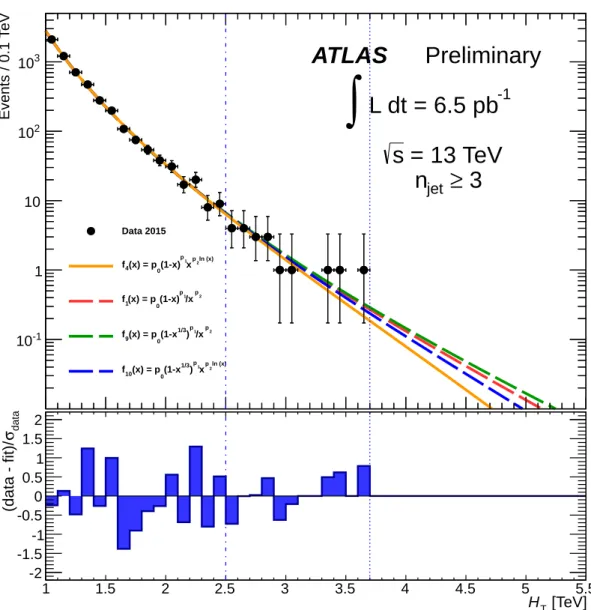
Figure 3 shows fits to the data in the control region and their extrapolation into the signal and validation regions for n

≥ 3 and the data set corresponding to the first step in the bootstrap. Function 4 is the baseline while functions 1, 9 and 10 pass the control region and monotonicty tests. The baseline is used to predict rates in the signal region and the remainder used to assess systematic uncertainties. As will be quantified below, but is already clear from this figure, there is no evidence for a discrepancy in the signal and validation regions between the data and the remaining extrapolations.

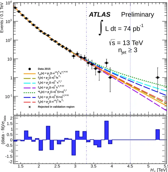
Figure 4 shows the comparison for the 74 pb

data set which corresponds to the second step. Here the functions 1, 3, 4, 5, 6, 9, and 10 are qualified for all jet multiplicities with 10 being the baseline.

Additionally, function 8 is qualified for n

≥ 4 - 7, function 7 for n

≥ 6 - 7, and function 2 for n

≥ 6.

5 Uncertainties

There are two components of uncertainty on the background projections: a statistical component arising

from data fluctuations in the control region and a systematic component associated with the choice and

extrapolation of the empirical fitting functions. In a pseudo-experiment based approach, the statistical

component and the extrapolation uncertainty of the baseline fitting function are estimated by the width

and median value of the difference between the extrapolations obtained from pseudo-experiments using

the baseline function and the actual values in the validation and signal regions of the H

distribution. In a

data-driven approach, the maximal difference in the background projection between the baseline function

E v e n ts / 0 .1 T e V

10

1 10 10

10

ATLAS Preliminary

L dt = 6.5 pb -1

∫

≥ 3 n jet

= 13 TeV s

Data 2015

ln (x) p2 1x

p

(1-x) (x) = p0

f4

p2

/x

p1

(1-x)

0

(x) = p f1

p2 1/x

p 1/3)

0(1-x (x) = p f9

ln (x) 2

xp p1 1/3)

0(1-x (x) = p f10

[TeV]

H

1 1.5 2 2.5 3 3.5 4 4.5 5 5.5

data

σ (data - fit)/

-2 -1.5 -1 -0.5 0 0.5 1 1.5 2

Figure 3: The data in 1.0 TeV < H

< 2.5 TeV for n

≥ 3 are fitted by the baseline function (solid), and three

alternative functions (dashed). The fitted functions are extrapolated to the validation region and signal region. The

control, validation and signal regions are delimited by the vertical lines. The bottom section of the figure shows

the residual significance defined as the ratio of the difference between fit and data over the statistical uncertainty of

data, where the fit prediction is taken from the baseline function.

E v e n ts / 0 .1 T e V

10

1 10 10

10

10

ATLAS Preliminary L dt = 74 pb -1

∫

≥ 3 n jet

= 13 TeV s

Data 2015

ln (x) p2

x

p1 1/3) (1-x

0

(x) = p f10

p2 1/x (1-x)p

(x) = p0

f1

2x

xp p1

(1-x) (x) = p0

f3

ln (x) p2 1x

p

(1-x) (x) = p0

f4

2x p

(1+x)

p1

(1-x) (x) = p0

*f5

ln (x) p2

(1+x)

p1

(1-x) (x) = p0

f6

p2 1/x )p

(1-x1/3 0

(x) = p f9

Rejected in validation region

[TeV]

H

1.5 2 2.5 3 3.5 4 4.5 5 5.5

data

σ (data - fit)/

-2 -1.5 -1 -0.5 0 0.5 1 1.5 2

Figure 4: The data in 1.2 TeV < H

< 3.2 TeV for n

≥ 3 are fitted by the baseline function (solid), and six

alternative functions (dashed). The fitted functions are extrapolated to the validation region and signal region. The

control, validation and signal regions are delimited by the vertical lines. The function indicated by an asterisk

is rejected at 95% CL by the data in the validation region. The bottom section of the figure shows the residual

significance defined as the ratio of the di ff erence between fit and data over the statistical uncertainty of data, where

the fit prediction is taken from the baseline function.

n

≥ VR (obs) VR (exp) SR (obs) SR (exp)

3 19 20.4 ± 4.4(PE) ± 2.6(DD) 0 0.65 ± 0.48(PE) ± 0.64 (DD) Table 2: The expected and observed number of events in the validation region (VR) and signal region (SR) are shown for n

≥ 3 in the 6.5 pb

data set. The uncertainties on the predicted rates are shown. They are obtained from the pseudo-experiment based approach (PE) and the data-driven approach (DD).

n

≥ VR (obs) VR (exp) SR (obs) SR (exp)

3 23 27.1 ± 3.7 (PE) ± 9.6 (DD) 1 1.42 ± 0.41 (PE) ± 4.3 (DD) 4 27 25.4 ± 3.2 (PE) ± 15.5 (DD) 0 1.62 ± 0.46 (PE) ± 9.2 (DD) 5 21 18.8 ± 2.9 (PE) ± 9.9 (DD) 0 1.32 ± 0.48 (PE) ± 5.0 (DD) 6 18 20.7 ± 3.3 (PE) ± 10.4 (DD) 0 1.19 ± 0.48 (PE) ± 13.3 (DD) 7 29 22.2 ± 3.7 (PE) ± 7.0 (DD) 0 0.81 ± 0.36 (PE) ± 0.60 (DD) Table 3: The expected and observed number of events in the validation region (VR) and signal region (SR) are shown for five overlapping inclusive jet multiplicity bins. The uncertainties on the predicted rates are shown. They are obtained from the pseudo-experiment based approach (PE) and the data-driven approach (DD).

and qualified alternate function is used to estimate the uncertainty associated with the choice of fitting function. The estimated uncertainties are shown in Tables 2 and 3 where they are indicated by (PE) and (data) based on the approach used.

The uncertainty on the expected signal yield includes a luminosity uncertainty of 9 % and jet energy scale and resolution uncertainties, which ranges from 1 to 4 % depending on the M

-M

values.

6 Results

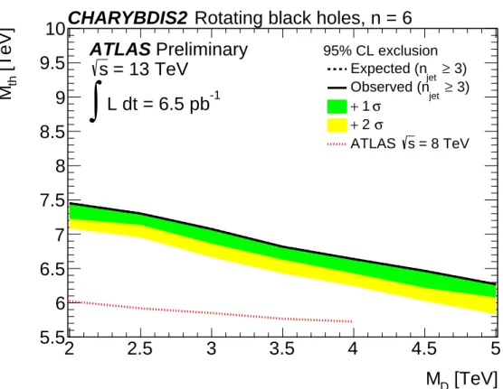
Table 2 shows the predicted number of background events in the validation and signal regions in the 6.5 pb

data for n

≥ 3. As already mentioned, the first step analysis is only performed with events with n

≥ 3. As can be seen from this table, the predicted and observed number of events in the validation regions are in agreement. There is no excess of events in the signal region and therefore a limit on the presence of new physics can be extracted. The modified frequentist C L

method [30] is used to set a 95% CL limit on the number of signal events. The model dependent 95% CL limit is shown as a function of M

and M

for CHARYBDIS2 using the n

≥ 3 result in Figure 5 for the data set with 6.5 pb

where it is compared with the Run-1 result. The expansion of limit contour enables a wider control region for the second step to be defined.

Table 3 shows the predicted number of background events in the validation and signal regions in the 74

pb

data set as a function of the inclusive jet multiplicity. In the case of n

≥ 3, function 5 fails in

the validation region, the remaining functions (10, 1, 4, 9, 6 and 3) are validated. These are shown in

Figure 4. For the remaining multiplicities all qualified functions are consistent with data in the validation

region and are used to obtain signal region estimates.

[TeV]

M D

2 2.5 3 3.5 4 4.5 5

[TeV] th M

5.5 6 6.5 7 7.5 8 8.5 9 9.5 10

ATLAS Preliminary L dt = 6.5 pb -1

∫ ^{s = 13 TeV}

95% CL exclusion

Rotating black holes, n = 6 CHARYBDIS2

≥ 3) Expected (n

≥ 3) Observed (n

σ + 1

σ + 2

= 8 TeV s

ATLAS

Figure 5: The expected and observed limits on the M

-M

grid, from the analysis with an integrated luminosity of 6.5 pb

. The 95% CL expected limit is shown as the black dashed line, and limits corresponding to the + 1 σ and + 2 σ variations of the background expectation are shown as the green and yellow bands, respectively. The 95%

CL observed limit is shown as the black solid line. The observed and expected limits are overlapped. The −1 σ and

−2 σ bands are not shown as they are degenerate with the expected limit. The red dotted line corresponds to the limit from Run-1 ATLAS multi-jet search [5].

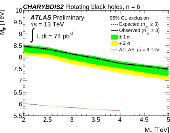
As can be seen from Table 3, no excess of events is observed in the signal regions, and therefore a limit on the presence of new physics can again be extracted. The limit is extracted using n

≥ 3 which has the best expected limit. The model dependent 95% limit is shown as a function of M

and M

for CHARYBDIS2 using the n

≥ 3 result in Figure 6 for the data set with 74 pb

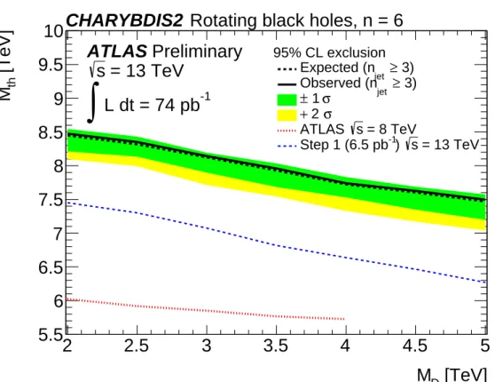
where it is compared with the Run- 1 result. The expected limit significantly exceeds the sensitivity reached by the Run-1 ATLAS search.

The observed limit is slightly tighter than the expected one, as an deficit with respect to the background prediction is observed in the signal region of n

≥ 3. The production of a rotating black hole with n = 6 is excluded, for M

up to 7.5 TeV - 8.5 TeV, depending on the M

.

7 Conclusion

A search for signals of strong gravity in multijet final states has been performed using 80 pb

of data

taken at 13 TeV using the ATLAS detector. No evidence for deviations from SM expectations have been

seen. In the CHARYBDIS2 1.0.4 model exclusions are shown as a function of M

and M

The production ˙

of a rotating black hole with n = 6 is excluded, for M

up to 7.5 TeV - 8.5 TeV, depending on the M

.

[TeV]

M D

2 2.5 3 3.5 4 4.5 5

[TeV] th M

5.5 6 6.5 7 7.5 8 8.5 9 9.5 10

ATLAS Preliminary L dt = 74 pb -1

∫ ^{s = 13 TeV}

95% CL exclusion

Rotating black holes, n = 6 CHARYBDIS2

≥ 3) Expected (n

≥ 3) Observed (n

σ

± 1 σ + 2

= 8 TeV s

ATLAS

Figure 6: The expected and observed limits on the M

-M

grid, from the analysis with an integrated luminosity of 74 pb

. The 95% CL expected limit is shown as the black dashed line, and limits corresponding to the ± 1 σ and + 2 σ variations of the background expectation are shown as the green and yellow bands, respectively. The 95%

CL observed limit is shown as the black solid line. The −2 σ band is not shown as it is degenerate with the −1 σ band. The red dotted line corresponds to the limit from Run-1 ATLAS multi-jet search [5].

These extend significantly the limits from the 8 TeV analyses.

References

[1] N. Arkani-Hamed, S. Dimopoulos and G. R. Dvali,

The Hierarchy problem and new dimensions at a millimeter, Phys. Lett. B429 (1998) 263–272, arXiv: hep-ph/9803315 [hep-ph].

[2] I. Antoniadis et al., New dimensions at a millimeter to a Fermi and superstrings at a TeV, Phys. Lett. B 436 (1998) 257–263, arXiv: hep-ph/9804398 [hep-ph].

[3] L. Randall and R. Sundrum, A large mass hierarchy from a small extra dimension, Phys. Rev. Lett. 83 (1999) 3370–3373, arXiv: hep-ph/9905221 [hep-ph].

[4] L. Randall and R. Sundrum, An alternative to compactification,

Phys. Rev. Lett. 83 (1999) 4690–4693, arXiv: hep-th/9906064 [hep-th].

[5] G. Aad et al., Search for low-scale gravity signatures in multi-jet final states with the ATLAS detector at √

s = 8 TeV, JHEP 07 (2015) 032, arXiv: 1503.08988 [hep-ex].

[6] ATLAS Collaboration, Search for strong gravity signatures in same-sign dimuon final states using the ATLAS detector at the LHC, Phys. Lett. B 709 (2012) 322–340, arXiv: 1111.0080 [hep-ex].

[7] ATLAS Collaboration, Search for microscopic black holes in a like-sign dimuon final state using large track multiplicity with the ATLAS detector, Phys. Rev. D 88 (2013) 072001,

arXiv: 1308.4075 [hep-ex].

[8] ATLAS Collaboration, Search for TeV-scale gravity signatures in final states with leptons and jets with the ATLAS detector at √

s = 7 TeV, Phys. Lett. B 716 (2012) 122–141, arXiv: 1204.4646 [hep-ex].

[9] ATLAS Collaboration, Search for microscopic black holes and string balls in final states with leptons and jets with the ATLAS detector at √

s = 8 TeV, J. High Energy Phys. 1408 (2014) 103, arXiv: 1405.4254 [hep-ex].

[10] CMS Collaboration, Search for microscopic black hole signatures at the Large Hadron Collider, Phys. Lett. B 697 (2011) 434–453, arXiv: 1012.3375 [hep-ex].

[11] CMS Collaboration, Search for microscopic black holes in pp collisions at √

s = 7 TeV, J. High Energy Phys. 1204 (2012) 061, arXiv: 1202.6396 [hep-ex].

[12] CMS Collaboration, Search for microscopic black holes in pp collisions at √

s = 8 TeV, J. High Energy Phys. 1307 (2013) 178, arXiv: 1303.5338 [hep-ex].

[13] J. A. Frost et al., Phenomenology of production and decay of spinning extra-dimensional black holes at hadron colliders, J. High Energy Phys. 0910 (2009) 014, arXiv: 0904.0979 [hep-ph].

[14] ATLAS Collaboration, The ATLAS experiment at the CERN Large Hadron Collider, J. Instrumentation 3 (2008) S08003.

[15] ATLAS Collaboration, Improved luminosity determination in pp collisions at √

s = 7 TeV using the ATLAS detector at the LHC, Eur. Phys. J. C 73 (2013) 2518, arXiv: 1302.4393 [hep-ex].

[16] M. Cacciari, G. P. Salam and G. Soyez, The anti-k

jet clustering algorithm, J. High Energy Phys. 0804 (2008) 063, arXiv: 0802.1189 [hep-ph].

[17] W. Lampl et al., Calorimeter clustering algorithms: description and performance,

ATL-LARG-PUB-2008-002 (2012), url : http://cdsweb.cern.ch/record/1099735.

[18] ATLAS Collaboration, Pile-up subtraction and suppression for jets in ATLAS, ATLAS-CONF-2013-083 (2013), url: http://cds.cern.ch/record/1570994.

[19] ATLAS Collaboration, Jet global sequential corrections with the ATLAS detector in proton-proton collisions at √

s = 8 TeV, ATLAS-CONF-2015-002 (2015), url : http://cds.cern.ch/record/2001682.

[20] ATLAS Collaboration, Data-driven determination of the energy scale and resolution of jets reconstructed in the ATLAS calorimeters using dijet and multijet events at √

s = 8 T eV , ATLAS-CONF-2015-017 (2015), url : http://cds.cern.ch/record/2008678.

[21] ATLAS Collaboration, Jet Calibration and Systematic Uncertainties for Jets Reconstructed in the ATLAS Detector at √

s = 13 TeV Draft CONF NOTE in preparation for EPS , ATL-COM-PHYS-2015-444 (2015), url : http://cds.cern.ch/record/2018215.

[22] T. Sjostrand, S. Mrenna and P. Z. Skands, A brief introduction to PYTHIA 8.1, Comput. Phys. Commun. 178 (2008) 852–867, arXiv: 0710.3820 [hep-ph].

[23] R. D. Ball et al., Parton distributions for the LHC Run II, JHEP 04 (2015) 040, arXiv: 1410.8849 [hep-ph].

[24] ATLAS Collaboration, Summary of ATLAS Pythia 8 tunes, ATL-PHYS-PUB-2012-003 (2012) 14, url : http://cds.cern.ch/record/1474107.

[25] H.-L. Lai et al., New parton distributions for collider physics, Phys. Rev. D 82 (2010) 074024, arXiv: 1007.2241 [hep-ph].

[26] S. Agostinelli et al., Geant4 - A simulation toolkit,

Nucl. Instrum. Methods Phys. Res. Sect. A 506.3 (2003) 250 –303, issn: 0168-9002.

[27] ATLAS Collaboration, The ATLAS simulation infrastructure,

Eur. Phys. J. C 70 (3 2010) 823–874, issn : 1434-6044, arXiv: 1005.4568 [physics].

[28] A. Martin et al., Parton distributions for the LHC, Eur. Phys. J. C 63 (2009) 189–285, arXiv: 0901.0002 [hep-ph].

[29] ATLAS Collaboration,

The simulation principle and performance of the ATLAS fast calorimeter simulation FastCaloSim, ATL-PHYS-PUB-2010-013 (2010) 14, url : http://cds.cern.ch/record/1300517.

[30] A. L. Read, Presentation of search results: The CL(s) technique, J. Phys. G 28 (2002) 2693–2704.

Additional material

E v e n ts / 0 .1 T e V

10

1 10 10

10

10

ATLAS Preliminary L dt = 74 pb -1

∫ s = 13 TeV

≥ 3 n jet

Data 2015

= 4 TeV = 7 TeV, MD

CHARYBDIS2 Mth

= 4 TeV = 7.5 TeV, MD

CHARYBDIS2 Mth ln (x) 2

xp p1 1/3)

0(1-x (x) = p f10

p2

/x

p1

(1-x)

0

(x) = p f1

x 2

xp p1

(1-x) (x) = p0

f3

ln (x) p2 1x

p

(1-x) (x) = p0

f4

2x p

(1+x)

p1

(1-x) (x) = p0

*f5

ln (x) p2

(1+x)

p1

(1-x) (x) = p0

f6

p2

/x

p1 1/3) (1-x

0

(x) = p f9

Rejected in validation region

[TeV]

H

2 3 4 5 6 7

data

σ (data - fit)/

-2 -1.5 -1 -0.5 0 0.5 1 1.5 2

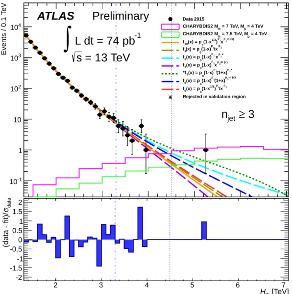
Figure 7: The data in 1.2 TeV < H

< 3.2 TeV for n

≥ 3 are fitted by the baseline function (solid), and six

alternative functions (dashed). The fitted functions are extrapolated to the validation region and signal region. The

control, validation and signal regions are delimited by the vertical lines. The function indicated by an asterisk

is rejected at 95% CL by the data in the validation region. The bottom section of the figure shows the residual

significance defined as the ratio of the difference between fit and data over the statistical uncertainty of data, where

the fit prediction is taken from the baseline function. The black hole signal distributions from Monte Carlo samples

at M

= 4 TeV, M

= 7.0 TeV and M

= 4 TeV, M

= 7.5 TeV are also shown.

[TeV]

M D

2 2.5 3 3.5 4 4.5 5

[TeV] th M

5.5 6 6.5 7 7.5 8 8.5 9 9.5 10

ATLAS Preliminary L dt = 74 pb -1

∫ ^{s = 13 TeV}

95% CL exclusion

Rotating black holes, n = 6 CHARYBDIS2

≥ 3) Expected (n

≥ 3) Observed (n

σ

± 1 σ + 2

= 8 TeV s

ATLAS

= 13 TeV s

-1

) Step 1 (6.5 pb

Figure 8: The expected and observed limits on the M

-M

grid, from the analysis with an integrated luminosity of 74 pb

. The 95% CL expected limit is shown as the black dashed line, and limits corresponding to the ± 1 σ and + 2 σ variations of the background expectation are shown as the green and yellow bands, respectively. The 95% CL observed limit is shown as the black solid line. The −2 σ band is not shown as it is degenerate with the

−1 σ band. The blue dashed line corresponds to the observed limit from the first step analysis. The red dotted line

corresponds to the limit from Run-1 ATLAS multi-jet search [5].