ATLAS NOTE ATLAS-CONF-2015-024

A TLAS-CONF-2015-024 06 July 2015

ATLAS NOTE

ATLAS-CONF-2015-024

6th July 2015

Measurement of the di ff erential cross-sections of prompt and non-prompt production of √ J /ψ and ψ (2S) in p p collisions at

s = 7 and 8 TeV with the ATLAS detector

The ATLAS Collaboration

Abstract

The production rates of prompt and non-prompt J/ψ and ψ(2S) mesons in their dimuon decay modes are measured using 2.1 fb

⁻¹

and 11.4 fb

⁻¹

of data collected with the ATLAS experiment at the Large Hadron Collider, in proton-proton collisions at √

s = 7 and 8 TeV.

Production cross-sections for both prompt and non-prompt sources, ratios of ψ(2S) to J/ψ production, and fractions of non-prompt to inclusive production for J/ψ and ψ(2S) are meas- ured as a function of meson transverse momentum and rapidity. The measurements are com- pared to theoretical predictions.

© 2015 CERN for the benefit of the ATLAS Collaboration.

Reproduction of this article or parts of it is allowed as specified in the CC-BY-3.0 license.

Contents

1 Introduction 2

2 The ATLAS Detector 4

3 Candidate selection 4

4 Methodology 5

4.1 Di ff erential cross-section determination 6

4.2 Non-prompt fraction 6

4.3 Ratio of ψ(2S) to J/ψ production in prompt and non-prompt production 7

4.4 Acceptance 7

4.5 Muon reconstruction and trigger e ffi ciency determination 8

4.6 Fitting Technique 9

4.7 Bin migration corrections 11

5 Systematic Uncertainties 12

6 Results 16

7 Conclusion 25

8 Average weight distributions 30

9 Projections of fit results 31

10 Prompt and non-prompt ratio, and non-prompt fraction results in two-dimensional plots 36

11 Comparison with other LHC experiments 37

1 Introduction

Measurements of heavy quark-antiquark bound states (quarkonia) production processes provide an insight into the nature of quantum chromodynamics (QCD) close to the boundary between the perturbative and non-perturbative regimes. More than forty years since the discovery of the J/ψ, the investigation of hidden heavy flavour production in hadronic collisions still presents significant challenges to both theory and experiment.

In high-energy hadronic collisions, charmonium states can be produced either directly by short-lived

QCD sources (“prompt” production), or by long-lived sources such as decays of beauty hadrons (“non-

prompt” production). These can be separated experimentally by measuring the distance between the

proton-proton primary interaction and the decay vertex of the quarkonium state. While Fixed-Order with

Next-to-Leading-Log (FONLL) calculations [1, 2], within the framework of perturbative QCD, have been

satisfactorily successful in describing the non-prompt contributions, a satisfactory understanding of the

prompt production mechanisms is still to be achieved.

The ψ(2S) meson is the only vector charmonium state that is produced with no significant contributions from decays of higher-mass quarkonia, referred to as feed-down contributions. This provides a unique opportunity to study production mechanisms specific to J

^PC

= 1

⁻⁻

states [3–12]. Measurements of the production of J

⁺⁺

states J = 0, 1, 2, [12–17], strongly coupled to the two-gluon channel, allow similar studies in that sector, essentially complementary to the vector sector. J/ψ production [3–7, 9–11, 13, 18–24] arises from a mixture of di ff erent sources, receiving contributions from the production of 1

⁻⁻

and J

⁺⁺

states in comparable amounts.

Early attempts to describe the charmonium formation [25–32] using leading-order perturbative QCD gave rise to a variety of models, none of which could explain the large production cross-sections measured at the Tevatron [3, 13, 21–23]. Within the colour-singlet model (CSM) [33] next-to-next-to-leading- order (NNLO) contributions to the hadronic production of S-wave quarkonia were calculated without introducing any new phenomenological parameters. However, technical di ffi culties have made it so far impossible to perform the full NNLO calculation, or to extend those calculations to the P-wave states, so it is not entirely surprising that the predictions of the model fall significantly below the experimental data for inclusive production of J/ψ and Υ states [18, 34].

Non-relativistic QCD (NRQCD) calculations that include colour-octet (CO) contributions [35] introduce a number of phenomenological parameters — long-distance matrix elements (LDMEs) — which are de- termined from fits to the experimental data, and can hence describe the cross-sections and di ff erential spectra satisfactorily well [36]. However, the attempts to describe the polarisation of S-wave quarkonium states using this approach have not been so successful [37], prompting a suggestion [38] that a more coher- ent approach is needed to the treatment of polarisation within the QCD-motivated models of quarkonium production.

Neither the CSM nor the NRQCD model give a satisfactory explanation for the measurement of prompt J/ψ production in association with the W [39] and Z [40] bosons: in both cases, the measured di ff erential cross-section is larger than theoretical expectations [41–44].

It is also important to broaden the scope of comparisons between theory and experiment by providing a variety of experimental information on quarkonium production across a wider kinematic range. In this context, ATLAS has measured the inclusive differential cross-section of J/ψ production at √

s = 7 TeV, using the data collected in 2010 with 2.3 pb

⁻¹

of integrated luminosity [18], as well as the di ff eren- tial cross-sections of the production of χ

_c

states (4.5 fb

⁻¹

) [14], and of the ψ (2S) in its J/ψππ decay mode (2.1 fb

⁻¹

) [9], at √

s = 7 TeV with data collected in 2011. The cross-section and polarisation measurements from CDF [4], CMS [4, 6, 45], LHCb [8, 10, 12, 46–48] and ALICE [5], cover a consider- able variety of charmonium production characteristics in a wide kinematic range (transverse momentum p

_T

≤ 100 GeV and rapidities of | y| < 5), thus providing a wealth of information for a new generation of theoretical models.

This paper presents a high-statistics measurement of J/ψ and ψ(2S) production in the dimuon decay mode, both at √

s = 7 TeV and at √

s = 8 TeV. It is presented as a double-differential measurement in

transverse momentum and rapidity of quarkonium, separated into prompt and non-prompt contributions,

covering a range of transverse momenta 8 < p

_T

≤ 110 GeV in rapidities out to |y | < 2.0. Also repor-

ted are the prompt and non-prompt ratios of ψ (2S) to J/ψ production, and the non-prompt production

fractions relative to those inclusively produced for both J/ψ and ψ

⁰

mesons.

2 The ATLAS Detector

The ATLAS experiment [49] is a general-purpose detector consisting of an inner tracker, a calorimeter and a muon spectrometer. The inner detector (ID) directly surrounds the interaction point; it consists of a silicon pixel detector, a semiconductor tracker and a transition radiation tracker, and is embedded in an axial 2T magnetic field. The ID coverage goes up to pseudo-rapidity 1 |η| = 2.5 and is enclosed by a calorimeter system containing electromagnetic and hadronic sections. The calorimeter is surrounded by a large muon spectrometer (MS) in a toroidal magnet system. The MS consists of monitored drift tubes and cathode strip chambers, designed to provide precise position measurements in the bending plane in the range |η | < 2.7. In addition, resistive plate chambers (RPCs) and thin gap chambers (TGCs) with a coarse position resolution but a fast response time are used to trigger muons in the ranges |η | < 1.05 and 1.05 < |η| < 2.4, respectively.

The ATLAS trigger system [50] has three levels: the hardware-based Level-1 trigger and the two-stage High Level Trigger (HLT), comprising the Level-2 trigger and Event Filter (EF), which reduce the 20 MHz proton-proton collision rate to a several-hundred Hz rate for transfer to mass storage. At Level-1, the muon trigger searches for patterns of hits satisfying di ff erent transverse momentum thresholds using the RPCs and TGCs. Around these Level-1 hit patterns “Regions-of-Interest” (RoI) are defined which serve as seeds for the HLT muon reconstruction.

3 Candidate selection

The analysis is based on data recorded at the LHC during proton–proton collisions at a centre-of-mass energy of 7 TeV and 8 TeV, collected in 2011 and 2012, respectively. This data sample corresponds to a total integrated luminosity of 2.1 fb

⁻¹

and 11.4 fb

⁻¹

for 7 TeV data and 8 TeV data, respectively.

Events were selected online using a trigger requiring two oppositely-charged muon candidates, each passing the requirement p

_T

> 4 GeV, and the muons are constrained to originate from a common vertex, which is fitted taking into account the track parameter uncertainties and a χ

²

/nd f cut from the vertex fit of 20 for the one degree of freedom is applied.

For the trigger used to collect data at 8 TeV, there was also a 4 GeV muon p

_T

threshold applied at Level- 1, which was not required for 7 TeV data and which modifies the trigger e ffi ciency profile at low muon transverse momenta towards lower values.

Events are selected by the offline analysis requiring at least two muons, identified by the muon spectro- meter with tracks reconstructed in the ID. Due to the ID acceptance, muon reconstruction is possible only for |η | < 2.5. The selected muons are further restricted to |η | < 2.3 ensuring high-quality tracking and triggering, and reducing the contribution from fake muons. For the momenta of interest in this analysis, measurements of the muons are degraded by multiple scattering within the MS and so only the inner

1

ATLAS uses a right-handed coordinate system with its origin at the nominal interaction point (IP) in the centre of the detector and the z-axis along the beam pipe. The x-axis points from the IP to the centre of the LHC ring, and the y-axis points upward. Cylindrical coordinates (r, φ) are used in the transverse plane, φ being the azimuthal angle around the beam pipe.

The pseudorapidity η is defined in terms of the polar angle θ as η = − ln tan(θ/2) and the transverse momentum p

_T

is defined as p

_T

= p sin θ. The rapidity is defined as y = 0.5 ln E + p

z

/ E − p

z

, where E and p

z

refer to energy and longitudinal momentum, respectively. The η–φ distance between two particles is defined as ∆R = q

(∆ η)

²

+ (∆ φ)

²

.

detector tracking information is considered. To ensure accurate inner detector measurements, each muon track must fulfill muon reconstruction performance selection requirements [51].

Muon candidates passing quality criteria are required to have opposite sign. A spatial matching re- quirement between each reconstructed muon candidate and the trigger identified candidates within a cone of ∆R = p

( ∆η )

²

+ ( ∆φ)

²

< 0.01 is required to accurately correct for trigger inefficiencies.

All dimuon candidates with an invariant mass, as determined from a fit to a common vertex, within 2.6 < m( µµ) < 4.0 GeV and within the kinematic range p

_T

( µµ) > 8 GeV, | y( µµ) | < 2.0 are retained for the analysis. In the case that multiple candidates are found in an event (occurring in approximately 10

⁻⁶

of selected events), all candidates are retained. The properties of the dimuon system, such as invariant mass m( µµ), transverse momentum p

_T

( µµ), and rapidity | y ( µµ) | are determined from the result of the fit.

4 Methodology

The measurements are performed in intervals of dimuon p

_T

and absolute value of the rapidity (| y |). The definition prompt refers to the J/ψ or ψ(2S) states — hereafter called ψ to refer to either — produced from short-lived QCD decays, including feed-down from other charmonium states as long as they are also produced from short-lived sources; if the decay chain producing a ψ state includes long-lived particles such as b-hadrons, then such ψ mesons are labelled as non-prompt. Using a simultaneous fit to the invariant mass of the dimuon and its decay time (described below), prompt and non-prompt signal and background contributions can be extracted from the data.

The probability for the decay of a particle as a function of proper decay time t follows an exponential distribution, p(t) = 1/τ

_B

· e

^−t/τB

where τ

_B

is the lifetime of the particle. For each decay, the proper decay time can be calculated as t = L/ βγ, where L is the distance between the particle production and decay point, β = v/c and γ is the Lorentz factor. As the non-prompt decays of ψ mesons do not fully reconstruct the b-hadron decay, the transverse momentum of the dimuon system, and the reconstructed dimuon invariant mass are used to construct the “pseudo-proper decay time”, τ = L

_{x y}

m( µµ)/p

_T

( µµ), where L

_{x y}

≡ ~ L · p ~

_T

( µµ)/p

_T

( µµ) is the signed projection of the distance of the dimuon decay vertex from the primary vertex, ~ L, onto its transverse momentum, p ~

_T^{(µ µ)}

. This is a good approximation to using the parent b-hadron information when the ψ and parent momenta are closely aligned, which is the case for the values of ψ transverse momenta considered here, and τ therefore can be used to statistically distinguish between the prompt and non-prompt processes.

If the event contains multiple primary vertices, the dimuon system is assigned to the primary vertex

closest in z to the decay vertex. The e ff ect of selecting an incorrect vertex has been shown [52] to have

a negligible impact on the extraction of prompt and non-prompt contributions. If any of the muons from

the dimuon candidate contributes to the construction of the primary vertex, the corresponding tracks are

removed and the vertex is refitted.

4.1 Di ff erential cross-section determination

Di ff erential dimuon prompt and non-prompt cross-sections times branching ratio for both the production of J/ψ or ψ(2S) mesons are measured separately according to the equations:

d

²

σ (pp → ψ)

dp

T

dy × B(ψ → µ

⁺

µ

⁻

) = N

_ψ^p

∆p

_T

∆ y × R

Ldt (1)

d

²

σ(pp → b b ¯ → ψ)

dp

_T

dy × B(ψ → µ

⁺

µ

⁻

) = N

_ψ^np

∆p

_T

∆ y × R

Ldt (2)

where R

L dt is the integrated luminosity, ∆p

_T

and ∆ y are the interval sizes in terms of dimuon transverse momentum and rapidity, respectively, and N

_ψ^p(np)

is the number of observed prompt or non-prompt J/ψ or ψ(2S) mesons in the slice under study, corrected for acceptance, trigger and reconstruction e ffi ciencies.

The intervals in ∆y combine the data from both negative and positive rapidities. These di ff erential cross- sections are determined separately for the J/ψ and ψ (2S) states.

The determination of the cross-sections proceeds in several steps. First, a weight is determined for each selected dimuon candidate equal to the inverse of the total e ffi ciency for each candidate. Second, a fit is performed to the distribution of weighted events using an unbinned maximum likelihood fit on the dimuon invariant mass, m( µµ), and pseudo-proper decay time, τ, observables, to determine the yields of J/ψ → µ

⁺

µ

⁻

and ψ (2S) → µ

⁺

µ

⁻

produced in each (p

_T

( µµ), | y( µµ) |) interval. These yields are determined separately for prompt and non-prompt processes. Finally, the differential cross-section times the ψ → µ

⁺

µ

⁻

branching fraction is calculated for each state by including the integrated luminosity and the p

_T

and rapidity interval widths as shown in Eq. (1) and (2).

The total weight, w

tot

, for each dimuon candidate includes three factors: the fraction of produced ψ → µ

⁺

µ

⁻

decays with both muons in the kinematic region p

_T

( µ) > 4 GeV and |η ( µ) | < 2.3 (defined as acceptance, A ), the probability that a candidate within the acceptance satisfies the offline reconstruction selection (

_reco

), and the probability that a reconstructed event satisfies the trigger selection (

_trig

). The weights assigned to a given candidate when calculating the cross-sections are then given by:

w

⁻¹_tot

= A ·

reco

·

trig

4.2 Non-prompt fraction

The non-prompt fraction is defined as number of non-prompt ψ (produced via the decay of a b-hadron) relative to the number of inclusively produced ψ decaying to muon pairs after applying weighting correc- tions:

f

_b^ψ

≡ pp → b + X → ψ + X

⁰

pp −−−−−−→

^Inclusive

ψ + X

⁰

= N

_ψ^np

N

_ψ^np

+ N

_ψ^p

where this fraction is determined separately for both J/ψ and ψ (2S). The use of the fraction is advantage-

ous since acceptance and e ffi ciencies are largely cancelled and the total systematic e ff ects are reduced.

4.3 Ratio of ψ(2S) to J /ψ production in prompt and non-prompt production The ratio of ψ (2S) to J/ψ production, in their dimuon decay modes, is defined as:

R

^p(np)

= N

_ψ(2S)^p(np)

N

_J/ψ^p(np)

where N

_ψ^p(np)

is the number of prompt (non-prompt) J/ψ or ψ(2S) mesons decaying into a muon pair in an interval, corrected for selection e ffi ciencies and acceptance.

For the ratio measurements, similarly to the non-prompt fraction, the acceptance and efficiency correc- tions largely cancel, thus allowing a more precise measurement. The theoretical uncertainties on such ratios are also smaller, as several dependencies, such as parton density functions and b-hadron production spectra, cancel in the ratio.

4.4 Acceptance

The kinematic acceptance A ( p

_T

, y) for a ψ → µ

⁺

µ

⁻

decay with p

_T

and y is given by the probability that both muons pass the fiducial selection (p

_T

( µ) > 4 GeV and |η ( µ) | < 2.3). This is calculated using generator-level simulations. Detector-level corrections, which are found to be small, are applied to the results and also considered as part of the systematic uncertainties.

The acceptance A depends on five independent variables (two muon momenta constrained by the m( µµ) mass condition), chosen as the p

_T

, | y| and azimuthal angle φ of the ψ meson in the laboratory frame, and two angles characterising the ψ → µ

⁺

µ

⁻

decay, θ

^?

and φ

^?

. The angle θ

^?

is the angle between the direction of the positive-muon momentum in the ψ rest frame, and the momentum of the ψ in the laboratory frame, while φ

^?

is defined as the angle between the dimuon production and decay planes in the laboratory frame. The ψ production plane is defined by the momentum of the ψ in the laboratory frame and the positive z axis direction. The distributions in θ

^?

and φ

^?

differ for various possible spin alignment scenarios of the dimuon system.

The spin-alignment of the ψ may vary depending on the production mechanism, which in turn a ff ects the angular distribution of the dimuon decay. Predictions of various theoretical models are quite contra- dictory, while the recent experimental measurements [7] indicate that the angular dependence of J/ψ and ψ(2S) decays is consistent with being isotropic. This analysis adopts the isotropic distribution in both cos θ

^?

and φ

^?

angles as nominal.

The coe ffi cients λ

θ

, λ

φ

, λ

θφ

in d

²

N

d cos θ

^?

dφ

^?

∝ 1 + λ

θ

cos

²

θ

^?

+ λ

φ

sin

²

θ

^?

cos 2φ

^?

+ λ

θφ

sin 2θ

^?

cos φ

^?

are related to the spin-density matrix elements of the dimuon spin wave function. The same technique has also been used in other measurements [9, 14, 34].

Seven extreme cases that lead to the largest possible variations of acceptance within the phase space of

this measurement are identified. These cases, described in Table 1, are used to define a range in which

the results may vary under any physically allowed spin-alignment assumptions.

Table 1: Values of angular coe ffi cients describing the considered spin-alignment scenarios.

Angular coe ffi cients λ

_θ

λ

_φ

λ

_θφ

Isotropic (central value) 0 0 0

Longitudinal −1 0 0

Transverse positive + 1 + 1 0

Transverse zero +1 0 0

Transverse negative +1 −1 0 O ff -(λ

θ

–λ

φ

)-plane positive 0 0 + 0.5 O ff -(λ

_θ

–λ

_φ

)-plane negative 0 0 −0.5

For each of the two mass-points (corresponding to the J/ψ and ψ (2S) masses), 2D maps are produced as a function of dimuon p

_T

( µµ) and | y( µµ) | for the set of spin-alignment hypotheses. Acceptance maps are defined within the range 8 < p

_T

( µµ) < 110 GeV, | y( µµ) | < 2.0, corresponding to the data considered in the analysis. The map is defined by 100 slices in | y( µµ) | and 4400 in p

_T

( µµ), using 200k trials for each point. The statistical uncertainty of each point is < 0.1% and is neglected. As the reconstructed candidates in the data cover a range of masses which is due in part to the detector resolution of the signal mesons and also from background contributions, the acceptance for a given candidate is interpolated linearly as a function of the reconstructed mass m( µµ) using the J/ψ and ψ (2S) known masses and acceptance maps.

Figure 1 shows the p

_T

acceptance projection for all the spin alignment hypotheses for the J/ψ meson, and also shows the ratio of acceptances for ψ (2S) to J/ψ mesons for the isotropic hypothesis.

[GeV]

T ψp J/

8 9 10 20 30 40 50 60 70 10²

AcceptanceψJ/

0 0.2 0.4 0.6 0.8 1

Isotropic (central value) Longitudinal Transverse positive Transverse zero Transverse negative

)-plane positive λφ

θ- λ Off-(

)-plane negative λφ

θ- λ Off-(

ATLAS Simulation Preliminary

)|

µ (µ

|y 0 0.25 0.5 0.75 1 1.25 1.5 1.75 2 ) [GeV]µµ(Tp

109 20 30 40 50 60 70 102

Acceptance Ratio

0.8 0.9 1 1.1 1.2 1.3 1.4 1.5 ATLAS Simulation Preliminary

Figure 1: Projections of the acceptance maps as a function of p

T

for the J/ψ meson (left) under the various spin alignment hypotheses. Ratio of acceptances for ψ(2S) to J/ψ (right), produced as a function of the dimuon p

T

and rapidity, where the central (isotropic) spin-alignment hypothesis has been assumed, and the muon selection criteria:

p

_T

(µ) > 4 GeV and |η (µ) | < 2.3 is applied.

4.5 Muon reconstruction and trigger e ffi ciency determination

The technique for correcting the data for trigger and reconstruction ine ffi ciencies is the same for the

7 TeV and 8 TeV data, and is described in [9, 34]. However, di ff erent e ffi ciency maps are required for

each set of data, and the 8 TeV corrections are detailed briefly below. For the 8 TeV data, the single-muon reconstruction efficiency is determined from a tag-and-probe study in dimuon decays [40]. The efficiency map is calculated as a function of p

_T

( µ) and q × η ( µ), where q = ±1 is the electrical charge of the muon, expressed in units of e.

The trigger efficiency correction consists of two components. The first part represents the trigger effi- ciency for a single muon in intervals of p

_T

( µ) and q × η ( µ). For the dimuon system there is a second correction to account for reductions in efficiency due to: closely spaced (in η–φ) muons firing only a single RoI, vertex quality cuts, and opposite sign requirements. This correction is performed in three rapidity intervals: 0–1.0, 1.0–1.2, 1.2–2.3. The correction is a function of ∆R( µµ) in the first two rapidity intervals and function of ∆R( µµ) and | y ( µµ) | in the last interval.

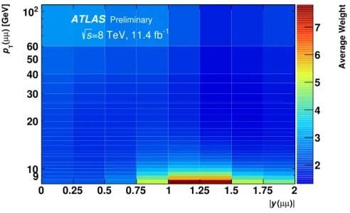
The final e ff ect of the combination of the two components (single muon e ffi ciency map and dimuon corrections) mentioned above is illustrated in Figure 2 in terms of p

_T

( µµ) and | y( µµ) |.

Average Weight

2 3 4 5 6 7

µ)|

(µ y

|

0 0.25 0.5 0.75 1 1.25 1.5 1.75 2

) [GeV]µµ( Tp

10 9 20 30 40 50 60 10

2

Preliminary

ATLAS

=8 TeV, 11.4 fb

-1

s

Figure 2: Average dimuon trigger weight in the intervals of p

_T

( µµ) and |y( µµ)| studied in this set of measurements.

4.6 Fitting Technique

The corrected prompt and non-prompt J/ψ and ψ (2S) signal yields are extracted from two-dimensional weighted unbinned maximum likelihood fits performed on the dimuon invariant mass (m( µµ)) and pseudo- proper decay time (τ) in each p

_T

( µµ) − |y ( µµ) | interval. Each interval is fitted independently with respect from all others. The probability density function (PDF) for each fit is defined as a normalized sum, where each term is factorized into mass and τ-dependent functions. The PDF can be written in a compact form as

PDF(m, τ) = X

7

i=1

κ

_i

f

_i

(m) · h

_i

(τ) ⊗ R( τ) (3) where κ

i

represents the relative normalisation of the i

^th

term (such that P

i

κ

i

= 1), f

_i

(m) is the mass-

dependent term, and ⊗ represents the convolution of the τ-dependent function h

_i

( τ) with the τ resolution

term, R(τ). The latter is modelled by a double Gaussian distribution with both means fixed to zero and widths determined from the fit.

Table 2 shows the contributions to the overall PDF with the corresponding f

_i

and h

_i

functions. Here G

₁

and G

2

are Gaussian, B

1

and B

2

are Crystal Ball distributions [53] (see below), while F is an uniform distribution and C

1

a first order Chebyshev polynomial. The exponential functions E

1

, E

2

, E

3

, E

4

and E

5

have di ff erent decay constants, where E

₅

( |τ|) is a double-sided exponential with the same decay constant on either side of τ = 0. The parameter ω represents the fractional contribution between the B and G mass signal contributions, while δ(τ) is used to represent the pseudo-proper decay time distribution of the prompt candidates.

Table 2: Description of the fit model PDF, see equation 3. Components of the probability density function used to extract the prompt (P) and non-prompt (NP) contributions for J/ψ and ψ (2S) signal and background (Bkg).

i Type Source f

_i

(m) h

_i

(τ)

1 J/ψ P ω B

₁

(m) + (1 − ω)G

₁

(m) δ(τ) 2 J/ψ NP ω B

₁

(m) + (1 − ω)G

₁

(m) E

₁

(τ) 3 ψ(2S) P ω B

₂

(m) + (1 − ω)G

₂

(m) δ(τ) 4 ψ(2S) NP ω B

₂

(m) + (1 − ω)G

₂

(m) E

₂

(τ)

5 Bkg P F δ(τ)

6 Bkg NP C

₁

(m) E

₃

(τ)

7 Bkg NP E

₄

(m) E

₅

( |τ|)

In order to make the fitting procedure more robust, a number of component terms share common para- meters to reduce the number of free parameters which led to 22 free parameters in total. In detail, the signal mass shapes are described by the sum of a Crystal Ball shape 2 (B) and Gaussian (G). For each of the J/ψ and ψ(2S), the B and G share a common mean, and freely determined widths, with the ratio between the B and G widths set to be common between the J/ψ and ψ (2S). The B parameters α, and n, describing the transition point of the low-edge from a Gaussian to a power-law shape, and the shape of the tail respectively, are fixed, and variations are considered as part of the fit model systematic uncertainties.

The width of G of the ψ (2S) is set to the width of the J/ψ multiplied by a free parameter scaling term.

The relative fraction of B and G is free, but common between the J/ψ and ψ(2S).

The non-prompt signal decay slopes (E

1

, E

₂

) are described by an exponential (for positive τ only) con- volved with a double Gaussian, R(τ) describing the pseudo-proper decay time resolution for the non- prompt component, and the same Gaussian response functions to describe the prompt contributions. Both resolution Gaussians have fixed means at τ = 0 and free widths. The decay constants of the J/ψ and ψ(2S) are separate free parameters in the fit.

The background contributions are described by a prompt and non-prompt component, as well as a double- sided exponential convolved with a double Gaussian describing mis-reconstructed or non-coherent dimuon pairs. The same resolution function as in signal is used to describe the background. For the non-resonant mass parameterizations, the non-prompt contribution is modelled by a first order Chebyshev polynomial.

2

The Crystal Ball function is given by:

B(x; α, n, x, σ) ¯ = N ·

 





 

 exp

−

^(x−x)¯2

2σ²

, for

^x−_σ^x¯

> − α A ·

A

⁰

−

^x−_σ^x¯

−n

, for

^x−_σ^x¯

6 −α where A =

_n

|α|

n

· exp

−

^|α|2

2

, A

⁰

=

_|αⁿ_|

− |α|

The prompt mass contribution follows a flat distribution and the double-sided background uses an expo- nential. Variations of this fit model are considered as systematical uncertainties.

The important quantities extracted from the fit are: fraction of events that are signal (prompt or non- prompt J/ψ or ψ (2S)); fraction of signal events that are prompt; fraction of prompt signal that is ψ(2S);

and fraction of non-prompt signal that is ψ(2S). From these parameters, and the weighted sum of events, all measured values are extracted.

For 7 TeV data, 168 fits are performed across the range of 8 < p

_T

< 100 GeV (8 < p

_T

< 60 GeV) for J/ψ (ψ (2S)) and 0 < | y| < 2. For 8 TeV data, 172 fits are performed across the range of 8 < p

_T

< 110 GeV and 0 < |y | < 2, excluding the area where p

_T

is less than 10 GeV and simultaneously | y | is greater than 0.75. This region is excluded due to a steeply changing low trigger efficiency and correlation effects which lead to an artificial fluctuation across rapidity of the measured cross-section.

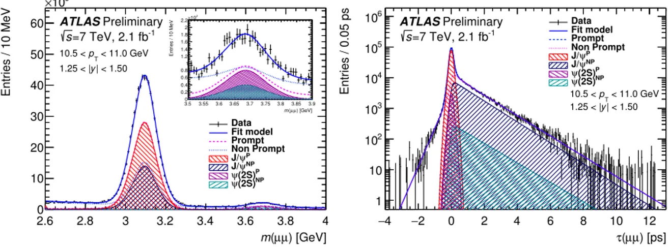
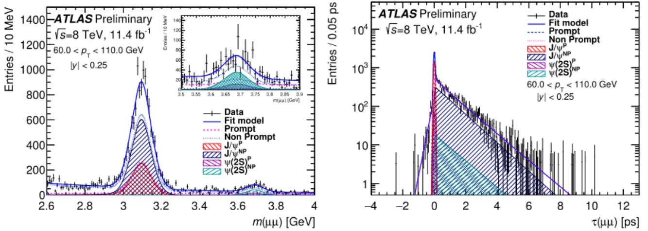
Figure 3 shows the fit results for one of the intervals considered in the analysis with the overall and individual contributions superimposed on the data, and projected onto the invariant mass and pseudo- proper decay time distributions for 7 TeV data. In Figure 4 the fit results are shown for one high-p

_T

interval of 8 TeV data.

) [GeV]

µ (µ m

2.6 2.8 3 3.2 3.4 3.6 3.8 4

Entries / 10 MeV

0 10 20 30 40 50 60

103

×

Data Fit model Prompt Non Prompt

ψP

J/ψNP

J/ _P (2S) ψ(2S)NP

ψ ATLASPreliminary

=7 TeV, 2.1 fb-1

s

< 11.0 GeV pT

10.5 <

| < 1.50 1.25 < |y

) [GeV]

µ (µ m 3.5 3.55 3.6 3.65 3.7 3.75 3.8 3.85 3.9

Entries / 10 MeV

0 0.2 0.4 0.6 0.8 1 1.2 1.4 1.6 1.8 2 2.2 103

×

) [ps]

µ (µ τ 4

− −2 0 2 4 6 8 10 12

Entries / 0.05 ps

1 10 102

103

104

105

106 _Data

Fit model Prompt Non Prompt

ψP

J/ψNP

J/(2S)P

ψ _NP (2S) ψ ATLASPreliminary

=7 TeV, 2.1 fb-1

s

< 11.0 GeV pT

10.5 <

| < 1.50 1.25 < |y

Figure 3: Projections of the fit result over the mass (left) and pseudo-proper decay time (right) distributions for data collected at 7 TeV for one typical interval. The data are in black, superimposed with the individual components of the fit result projections, where the total prompt and non-prompt components are represented by the dashed and dotted lines, respectively, and the shaded areas show the signal ψ prompt and non-prompt contributions.

4.7 Bin migration corrections

In order to account for bin migrations due to the detector resolution, corrections in the dimuon system p

_T

are derived by comparing analytic functions fit to the p

_T

spectra of dimuon events in data with and without convolution by the experimental resolution in p

_T

(determined from the fitted mass resolution and measured muon angular resolutions), as described in [34].

The numbers of acceptance and e ffi ciency-corrected dimuon decays extracted from the fits in each p

_T

and

rapidity interval are corrected for the differences between the true and reconstructed values of the dimuon

p

_T

. The correction factors, applied to the fitted yields deviate from unity by no more that 1.5%, and for

) [GeV]

µ (µ m

2.6 2.8 3 3.2 3.4 3.6 3.8 4

Entries / 10 MeV

0 200 400 600 800 1000 1200 1400

DataFit model Prompt Non Prompt

ψP

J/ψNP

J/(2S)P

ψ _NP (2S) ψ ATLASPreliminary

=8 TeV, 11.4 fb-1

s

< 110.0 GeV pT

60.0 <

| < 0.25 |y

) [GeV]

µ (µ m 3.5 3.55 3.6 3.65 3.7 3.75 3.8 3.85 3.9

Entries / 10 MeV

0 20 40 60 80 100 120 140

) [ps]

µ (µ τ

−4 −2 0 2 4 6 8 10 12

Entries / 0.05 ps

1 10 102

103

104

Data Fit model Prompt Non Prompt

ψP

J/ψNP

J/ _P ψ(2S)_NP

(2S) ψ ATLASPreliminary

=8 TeV, 11.4 fb-1

s

< 110.0 GeV pT

60.0 <

| < 0.25 |y

Figure 4: Projections of the fit result over the mass (left) and pseudo-proper decay time (right) distributions for data collected at 8 TeV an interval of high-p

_T

. The data are in black, superimposed with the individual components of the fit result projections, where the total prompt and non-prompt components are represented by the dashed and dotted lines, respectively, and the shaded areas show the signal ψ prompt and non-prompt contributions.

the majority of slices are smaller than 1%. The ratio measurement and non-prompt fractions are corrected by the corresponding ratios of bin migration correction factors. Using a similar technique, bin-migration corrections as a function of |y | are found to di ff er from unity by negligible amounts.

5 Systematic Uncertainties

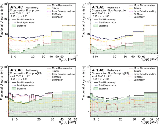
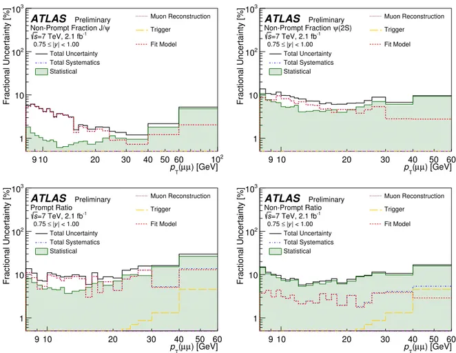
The considered sources of systematic uncertainties along with the minimum, maximum and median val- ues in percentage are listed in Table 3. The impact of these uncertainties to the production cross section measurements, as well as to the their ratios for 7 TeV (8 TeV have very similar behavior), is shown for a representative interval in Figure 5 and 6, respectively.

Table 3: Summary of the minimum and maximum contributions along with the median of the systematic uncertain- ties as percentages. Maximum values are quoted for 7 and 8 TeV.

7 TeV [%] 8 TeV [%]

Systematic Type Min Median Max Min Median Max

Luminosity 1.8 1.8 1.8 2.8 2.8 2.8

Inner Detector tracking e ffi ciency 1.0 1.0 1.0 1.0 1.0 1.0 Muon reconstruction e ffi ciency 0.7 1.2 4.7 0.3 0.7 6.0

Muon trigger efficiency 3.2 4.7 35.9 2.9 7.0 23.4

Fit model parameterizations 0.9 3.7 39.1 0.9 3.7 86.2

Bin migrations 0.01 0.1 1.4 0.01 0.3 1.5

Total 4.3 7.4 43.2 5.2 9.1 87.1

Luminosity

The uncertainty on the integrated luminosity is 1.8% (2.8%) for the 7 TeV (8 TeV) data-taking period.

) [GeV]

µ (µ pT

9 10 20 30 40 50 60 10²

Fractional Uncertainty [%]

1 10 102

103

ATLAS

Preliminary

=7 TeV, 2.1 fb-1

s

Cross-section Prompt J/ψ

| < 1.00 |y 0.75 ≤

Muon Reconstruction Trigger

Inner Detector tracking Fit Model

Luminosity Total Uncertainty

Total Systematics Statistical

) [GeV]

µ (µ pT

9 10 20 30 40 50 60 10²

Fractional Uncertainty [%]

1 10 102

103

ATLAS

Preliminary

=7 TeV, 2.1 fb-1

s

Cross-section Non-Prompt J/ψ

| < 1.00 |y 0.75 ≤

Muon Reconstruction Trigger

Inner Detector tracking Fit Model

Luminosity Total Uncertainty

Total Systematics Statistical

) [GeV]

µ (µ pT

9 10 20 30 40 50 60

Fractional Uncertainty [%]

1 10 102

103

ATLAS

Preliminary

=7 TeV, 2.1 fb-1

s

(2S) Cross-section Prompt ψ

| < 1.00 |y 0.75 ≤

Muon Reconstruction Trigger

Inner Detector tracking Fit Model

Luminosity Total Uncertainty

Total Systematics Statistical

) [GeV]

µ (µ pT

9 10 20 30 40 50 60

Fractional Uncertainty [%]

1 10 102

103

ATLAS

Preliminary

=7 TeV, 2.1 fb-1

s

(2S) Cross-section Non-Prompt ψ

| < 1.00 |y 0.75 ≤

Muon Reconstruction Trigger

Inner Detector tracking Fit Model

Luminosity Total Uncertainty

Total Systematics Statistical

Figure 5: Statistical and systematic contributions to the fractional uncertainty on the prompt (left column) and non-prompt (right column) J/ψ (top row) and ψ(2S) (bottom row) cross-sections for 7 TeV, shown for the region 0.75 < | y| < 1.00.

The methodology used to determine these uncertainties is described in [54]. The luminosity uncertainty is only applied to the J/ψ and ψ (2S) cross-section results.

Muon reconstruction and trigger e ffi ciencies

To determine the systematic uncertainty on the muon reconstruction and trigger e ffi ciency maps, each of the maps is reproduced in 100 pseudo-experiments. For each pseudo-experiment a new map is created by varying independently each bin content according to a Gaussian distribution about its estimated value, determined from the original map. In each pseudo-experiment, the total weight is recalculated for each dimuon p

_T

and | y| interval of the analysis. The RMS of the total weight pseudo-experiment distributions for each efficiency type is used as the systematic uncertainty.

The ID tracking e ffi ciency is in excess of 99.5%, and an uncertainty of 1% is applied to account for the inner detector reconstruction efficiency (0.5% per muon, added coherently). This uncertainty is applied to the differential cross-sections and is assumed to cancel in the fractions of non-prompt to inclusive production for J/ψ and ψ (2S) and ratios of ψ (2S) to J/ψ production.

For the trigger efficiency

_trig

, there is an additional correction that accounts for correlations between

) [GeV]

µ (µ pT

9 10 20 30 40 50 60 10²

Fractional Uncertainty [%]

1 10 102

103

ATLAS

Preliminary

=7 TeV, 2.1 fb-1

s

Non-Prompt Fraction J/ψ

| < 1.00 |y 0.75 ≤

Muon Reconstruction Trigger

Fit Model Total Uncertainty

Total Systematics Statistical

) [GeV]

µ (µ pT

9 10 20 30 40 50 60

Fractional Uncertainty [%]

1 10 102

103

ATLAS

Preliminary

=7 TeV, 2.1 fb-1

s

(2S) Non-Prompt Fraction ψ

| < 1.00 |y 0.75 ≤

Muon Reconstruction Trigger

Fit Model Total Uncertainty

Total Systematics Statistical

) [GeV]

µ (µ pT

9 10 20 30 40 50 60

Fractional Uncertainty [%]

1 10 102

103

ATLAS

Preliminary

=7 TeV, 2.1 fb-1

s

Prompt Ratio

| < 1.00 |y 0.75 ≤

Muon Reconstruction Trigger

Fit Model Total Uncertainty

Total Systematics Statistical

) [GeV]

µ (µ pT

9 10 20 30 40 50 60

Fractional Uncertainty [%]

1 10 102

103

ATLAS

Preliminary

=7 TeV, 2.1 fb-1

s

Non-Prompt Ratio

| < 1.00 |y 0.75 ≤

Muon Reconstruction Trigger

Fit Model Total Uncertainty

Total Systematics Statistical

Figure 6: Breakdown of the contributions to the fractional uncertainty on the non-prompt fractions for J/ψ (top left) and ψ (2S) (top right), and the prompt (bottom left) and non-prompt (bottom right) ratios for 7 TeV, shown for the region 0.75 < |y| < 1.00.

the two trigger muons. This correction is varied by its uncertainty, and the shift in the resultant total weight relative to its central value is added in quadrature to the uncertainty from the map. The choice of triggers is known [55] to introduce a small lifetime-dependent efficiency loss but is determined to have a negligible effect on the prompt and non-prompt yields and no correction is applied to this analysis.

Fit model systematics

The uncertainty due to the fit procedure was determined by varying one component at a time in the fit model described in section 4.6, creating a set of new fit models. For each new fit model, all measured quantities were recalculated, and in each p

_T

and | y | interval the maximal variation from the central fit model was used as its systematic uncertainty.

Variations to the central model fit were considered as:

• Signal model mass shape: using double Gaussians in place of the Crystal Ball plus Gaussian model;

and varying the α and n parameters of the B model, which are originally fixed.

• Signal model decay time shape: a double exponential was used to describe the decay time distribu- tion for the ψ non-prompt signal.

• Background mass shapes: varying the mass model using exponentials, quadratic Chebyshev poly- nomial to describe the components of prompt, non-prompt and double-sided background terms.

• Background decay time shape: for the non-prompt component, a single exponential was considered.

• Decay time resolution: using a single Gaussian in place of the double Gaussian to model the lifetime resolution (also prompt lifetime shape); and varying the mixing terms for the two Gaussians for the measurement.

Bin migrations

As the corrections to the results due to bin migration e ff ects are close to unity in all regions, the di ff erence between the correction factor and unity is applied as the uncertainty.

Fit model closure test

Closure tests were performed in order to validate the fit model. In these tests, two reconstructed Monte- Carlo samples were used that passed same reconstruction procedure as real data, one of them containing prompt J/ψ and the other containing non-prompt J/ψ coming from b-decays. In order to validate the fit model, 25 random fits were performed. On each fit, a dummy sample was created with varying composi- tions of prompt and non-prompt J/ψ originated from the Monte-Carlo samples mentioned above. The fit was performed on that sample and the estimated number of prompt and non-prompt events was compared with the real one. The results of the closure test can be seen in Figure 7, where the fractional difference between the truth and the estimated number of entries for prompt (dashed line) and non-prompt (continu- ous line) are less than 5% and are in satisfactorily agreement within the fitted statistical uncertainties to the truth values.

Fractional Difference

−0.2 −0.15 −0.1 −0.05 0 0.05 0.1 0.15 0.2

Entries

0 2 4 6 8 10 12 14 16 18 20 22

Prompt Non-Prompt ATLAS

Simulation Preliminary

Figure 7: Results of the closure test of the fit model. The fractional difference between the true and the estimated

number of entries for prompt (dashed line) and non-prompt (continuous line) contributions.

6 Results

The J/ψ and ψ(2S) non-prompt and prompt production cross-sections are presented, corrected for ac- ceptance and detector e ffi ciencies under the assumption of isotropic decays, as described in 4.1. Also presented are the fractions of non-prompt decays relative to all decays of J/ψ and ψ (2S) mesons, de- scribed here 4.2 and the ratio of prompt and non-prompt decays of ψ (2S) to J/ψ, described here 4.3. All the results presented have been derived using an unpolarised spin-alignment scenario.

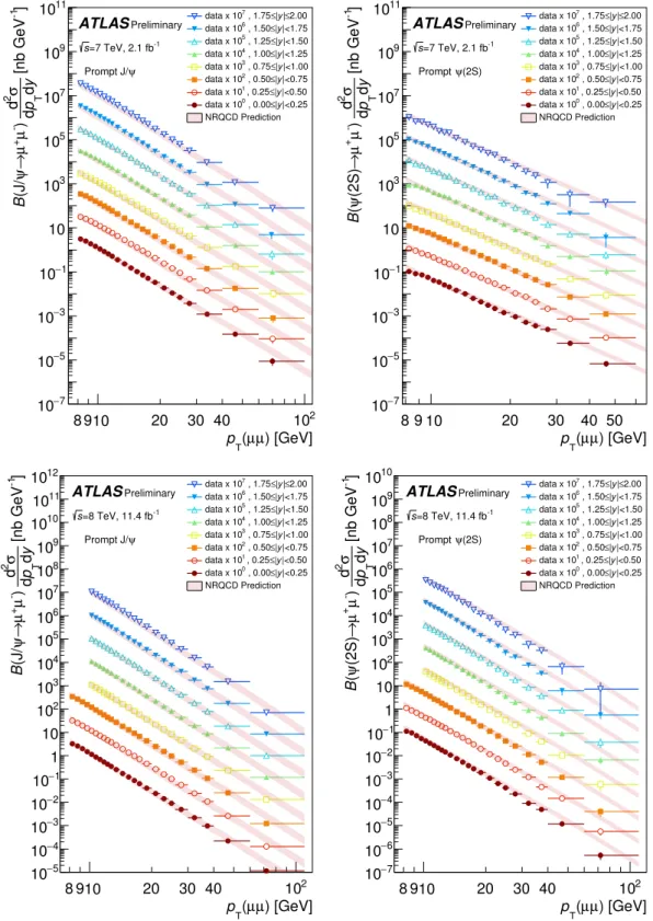
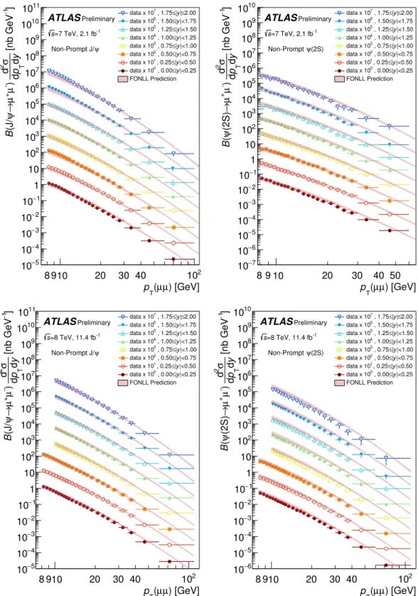
Production cross-sections

All production cross-sections presented in this section are corrected for acceptance and detector effi- ciencies with the assumption of isotropic decays, as described in section 4.1. Figures 8 and 9 show respectively the prompt and non-prompt di ff erential cross-sections of J/ψ and ψ (2S) as functions of p

_T

and | y| , together with the relevant theoretical predictions.

Non-prompt production fractions

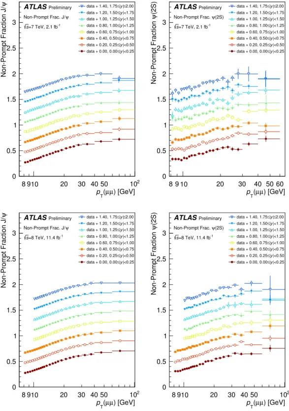
The results for the fractions of non-prompt decays relative to all decays of J/ψ and ψ (2S) presented as a function of p

_T

for slices of rapidity in Figure 10. In each rapidity slice, the non-prompt fraction is seen to increase as a function of p

_T

and has no strong dependence on either rapidity or center-of-mass energy.

Production ratios of ψ(2S) to J/ψ

The results of the fits for the ratio of ψ (2S) to J/ψ decaying to a muon pair and produced in prompt

and non-prompt processes are presented as a function of p

_T

for slices of rapidity in Figure 11. The non-

prompt ratio is shown to be relatively flat across the considered range of p

_T

, for each slice of rapidity. For

the prompt ratio, an increase as a function of p

_T

is observed, with no strong dependence on rapidity or

centre-of-mass energy.

) [GeV]

µ ( µ p

T

8 910 20 30 40 10

²

]

-1

[nb GeV y d

T

p d σ

2

d )

-

µ

+

µ → ψ (J/ B

7

10

−

−5

10

3

10

− 1

10

−

10 10

3

10

5

10

7

10

9

10

11 data x 107 _{, 1.75≤|y|≤2.00}

|<1.75 y

| , 1.50≤ data x 106

|<1.50 y

| , 1.25≤ data x 105

|<1.25 y

≤| , 1.00 data x 104

|<1.00 y

| , 0.75≤ data x 103

|<0.75

|y , 0.50≤ data x 102

|<0.50 y

| , 0.25≤ data x 101

|<0.25 y

| , 0.00≤ data x 100

NRQCD Prediction

ATLAS

Preliminary

=7 TeV, 2.1 fb-1

s Prompt J/ψ

) [GeV]

µ ( µ p

T

8 9 10 20 30 40 50

]

-1

[nb GeV y d

T

p d σ

2

d )

-

µ

+

µ → (2S) ψ ( B

7

10

−

−5

10

3

10

− 1

10

−

10 10

3

10

5

10

7

10

9

10

11 data x 107 _{, 1.75≤|y|≤2.00}

|<1.75 y

| , 1.50≤ data x 106

|<1.50 y

| , 1.25≤ data x 105

|<1.25 y

≤| , 1.00 data x 104

|<1.00 y

| , 0.75≤ data x 103

|<0.75

|y , 0.50≤ data x 102

|<0.50 y

| , 0.25≤ data x 101

|<0.25 y

| , 0.00≤ data x 100

NRQCD Prediction

ATLAS

Preliminary

=7 TeV, 2.1 fb-1

s ψ(2S) Prompt

) [GeV]

µ ( µ p

T

8 910 20 30 40 10

²

]

-1

[nb GeV y d

T

p d σ

2

d )

-

µ

+

µ → ψ (J/ B

−5

10

4

10

− 3

10

−

−2

10

1

10

−

1 10 10

2

10

3

10

4

10

5

10

6

10

7

10

8

10

9

10

10

10

11

10

12 _{data x 10}⁷ _{, 1.75≤|y|≤2.00}

|<1.75 y

| , 1.50≤ data x 106

|<1.50

|y , 1.25≤ data x 105

|<1.25 y

| , 1.00≤ data x 104

|<1.00 y

| , 0.75≤ data x 103

|<0.75 y

≤| , 0.50 data x 102

|<0.50 y

| , 0.25≤ data x 101

|<0.25 y

≤| , 0.00 data x 100

NRQCD Prediction

ATLAS

Preliminary

=8 TeV, 11.4 fb-1

s Prompt J/ψ

) [GeV]

µ ( µ p

T

8 910 20 30 40 10

²

]

-1

[nb GeV y d

T

p d σ

2

d )

-

µ

+

µ → (2S) ψ ( B

7

10

−

−6

10

5

10

−

−4

10

−3

10

−2

10

−1

10 1 10 10

2

10

3

10

4

10

5

10

6

10

7

10

8

10

9

10

10 _{data x 10}⁷ _{, 1.75≤|y|≤2.00}

|<1.75 y

| , 1.50≤ data x 106

|<1.50

|y , 1.25≤ data x 105

|<1.25 y

| , 1.00≤ data x 104

|<1.00 y

| , 0.75≤ data x 103

|<0.75 y

≤| , 0.50 data x 102

|<0.50 y

| , 0.25≤ data x 101

|<0.25 y

≤| , 0.00 data x 100

NRQCD Prediction

ATLAS

Preliminary

=8 TeV, 11.4 fb-1

s

(2S) Prompt ψ

Figure 8: The differential prompt cross-section times dimuon branching fraction of J/ψ (left) and ψ(2S) (right) as a

function of p

T

for each slice of rapidity. Top row is representing the 7 TeV results while bottom row the 8 TeV. For

each increasing rapidity slice, an additional scaling factor of 10 is applied to the plotted points for visual clarity. The

center of each bin on the horizontal axis represents the mean of the weighted p

_T

distribution. The horizontal error-

bars represent the range of p

_T

for the bin, and the vertical error-bar covers the statistical and systematic uncertainty

(with the same multiplicative scaling applied). Along with the measurements the NLO NRQCD theory predictions

) [GeV]

µ ( µ p

T

8 910 20 30 40 10

²

]

-1

[nb GeV y d

T

p d σ

2

d )

-

µ

+

µ → ψ (J/ B

−5

10

−4

10

−3

10

−2

10

−1

10 1 10 10

2

10

3

10

4

10

5

10

6

10

7

10

8

10

9

10

10

10

11 data x 107 _{, 1.75≤|y|≤2.00}

|<1.75 y

| , 1.50≤ data x 106

|<1.50 y

| , 1.25≤ data x 105

|<1.25 y

≤| , 1.00 data x 104

|<1.00 y

| , 0.75≤ data x 103

|<0.75

|y , 0.50≤ data x 102

|<0.50 y

| , 0.25≤ data x 101

|<0.25 y

| , 0.00≤ data x 100

FONLL Prediction

ATLAS

Preliminary

=7 TeV, 2.1 fb-1

s

Non-Prompt J/ψ

) [GeV]

µ ( µ p

T

8 9 10 20 30 40 50

]

-1

[nb GeV y d

T

p d σ

2

d )

-

µ

+

µ → (2S) ψ ( B

7

10

−

−6

10

5

10

−

−4

10

−3

10

−2

10

−1

10 1 10 10

2

10

3

10

4

10

5

10

6

10

7

10

8

10

9

10

10 data x 107 _{, 1.75≤|y|≤2.00}

|<1.75 y

| , 1.50≤ data x 106

|<1.50 y

| , 1.25≤ data x 105

|<1.25 y

≤| , 1.00 data x 104

|<1.00 y

| , 0.75≤ data x 103

|<0.75

|y , 0.50≤ data x 102

|<0.50 y

| , 0.25≤ data x 101

|<0.25 y

| , 0.00≤ data x 100

FONLL Prediction

ATLAS

Preliminary

=7 TeV, 2.1 fb-1

s

ψ(2S) Non-Prompt

) [GeV]

µ ( µ p

T

8 910 20 30 40 10

²

]

-1

[nb GeV y d

T

p d σ

2

d )

-

µ

+

µ → ψ (J/ B

−5

10

−4

10

3

10

− 2

10

−

−1

10 1 10 10

2

10

3

10

4

10

5

10

6

10

7

10

8

10

9

10

10

10

11 _{data x 10}⁷ _{, 1.75≤|y|≤2.00}

|<1.75 y

| , 1.50≤ data x 106

|<1.50

|y , 1.25≤ data x 105

|<1.25 y

| , 1.00≤ data x 104

|<1.00 y

| , 0.75≤ data x 103

|<0.75 y

≤| , 0.50 data x 102

|<0.50 y

| , 0.25≤ data x 101

|<0.25 y

≤| , 0.00 data x 100

FONLL Prediction

ATLAS

Preliminary

=8 TeV, 11.4 fb-1

s

Non-Prompt J/ψ

) [GeV]

µ ( µ p

T

8 910 20 30 40 10

²

]

-1

[nb GeV y d

T

p d σ

2

d )

-

µ

+

µ → (2S) ψ ( B

−6

10

−5

10

−4

10

−3

10

−2

10

−1

10 1 10 10

2

10

3

10

4

10

5

10

6

10

7

10

8

10

9

10

10 _{data x 10}⁷ _{, 1.75≤|y|≤2.00}

|<1.75 y

| , 1.50≤ data x 106

|<1.50

|y , 1.25≤ data x 105

|<1.25 y

| , 1.00≤ data x 104

|<1.00 y

| , 0.75≤ data x 103

|<0.75 y

≤| , 0.50 data x 102

|<0.50 y

| , 0.25≤ data x 101

|<0.25 y

≤| , 0.00 data x 100

FONLL Prediction

ATLAS

Preliminary

=8 TeV, 11.4 fb-1

s

(2S) Non-Prompt ψ

Figure 9: The differential non-prompt cross-section times dimuon branching fraction of J/ψ (left) and ψ(2S) (right) as a function of p

T

for each slice of rapidity. Top row is representing the 7 TeV results while bottom row the 8 TeV. For each increasing rapidity slice, an additional scaling factor of 10 is applied to the plotted points for visual clarity. The center of each bin on the horizontal axis represents the mean of the weighted p

_T

distribution.

The horizontal error-bars represent the range of p

_T

for the bin, and the vertical error-bar covers the statistical and

systematic uncertainty (with the same multiplicative scaling applied). Along with the measurements the FONLL