ATLAS-CONF-2013-094 03/09/2013
ATLAS NOTE
ATLAS-CONF-2013-094
September 3, 2013
Cross-Section Measurement of ψ(2S) → J/ψ(→ µ
+µ
−)π
+π
−in
√ s = 7 TeV pp Collisions at ATLAS
The ATLAS Collaboration
Abstract
The prompt and non-prompt production cross-sections forψ(2S) mesons are measured using 2.1 fb−1 ofppcollision data at a centre-of-mass energy of 7 TeV recorded by the ATLAS experiment at the LHC. The measurement studies the ψ(2S) → J/ψ(→ µ+µ−)π+π− decay mode, and probes ψ(2S) with transverse momenta in the range pT = 10−100 GeV and rapidity|y|<2.0. The results are compared to existing LHCψ(2S) production measurements and theoretical models for prompt and non-prompt production.
c
Copyright 2013 CERN for the benefit of the ATLAS Collaboration.
Reproduction of this article or parts of it is allowed as specified in the CC-BY-3.0 license.
1 Introduction
The production of quarkonium states in hadronic collisions has been the subject of intense theoretical and experimental study for many decades, especially since measurements of prompt
J/ψand
Υproduction at the Tevatron [1, 2, 3, 4] exposed order-of-magnitude differences between theoretical expectations and data. Despite these being among the most studied heavy quark bound states, there is still no complete understanding of the underlying production mechanisms and properties of formation. Quarkonium pro- duction acts as a unique and important testing ground for Quantum Chromodynamics (QCD) in its own right. While the production of a heavy quark pair occurs at a hard scale and is generally well-described by QCD, its subsequent evolution into a bound state includes many non-perturbative e
ffects at much softer scales that pose a challenge to current theoretical techniques. With the data obtained from the Large Hadron Collider (LHC), it is possible to make stringent tests of existing theoretical models across a large range of momentum transfer.
Studies on heavy quarkonium have previously been conducted at ATLAS with production measure- ments in the
J/ψ →µ
+µ
−[5] and
Υ(nS )
→µ
+µ
−[6, 7] modes. The measurements described here are based on an analysis of 2.1 fb
−1of
ppcollision data at
√s=
7 TeV, studying the prompt and non-prompt production of the ψ(2S) meson in the decay mode
J/ψ(→µ
+µ
−)π
+π
−, where the prompt production arises from direct QCD production mechanisms and the non-prompt production arises from weak decays of
b-hadrons. Unlike prompt J/ψproduction, which can occur through either direct QCD production of
J/ψor the production of excited
P-waveχ
cJstates that subsequently decay into
J/ψ+Xfinal states, the prompt production of ψ(2S) only proceeds through direct production. The measurement presented here, combined with a concurrent measurement of the prompt and non-prompt production of χ
cJ(nP) states [8] and with existing measurements of the production cross-section of the
J/ψ[5], serve to provide an accurate picture of the production of both prompt and non-prompt charmonium production.
The ψ(2S) cross-sections measured here are compared with the results from LHCb [9] and CMS [10]
and with a variety of theoretical models for both prompt and non-prompt production.
2 The ATLAS Detector
The ATLAS detector [11] is composed of an inner tracking system, calorimeters, and a muon spectrom- eter. The inner detector (ID) surrounds the proton-proton collision point and consists of a silicon pixel detector, a silicon microstrip detector, and a transition radiation tracker, all of which are immersed in a 2 T axial magnetic field. The inner detector spans the pseudorapidity
1range
|η|< 2.5 and is enclosed by a system of electromagnetic and hadronic calorimeters. Surrounding the calorimeters is the large muon spectrometer (MS). This spectrometer is equipped with monitored drift tubes and cathode strip chambers that provide precision measurements in the bending plane within the pseudorapidity range
|η|< 2.7. Re- sistive plate and thin gap chambers with fast response are additionally used primarily to make fast event data-recording decisions in the ranges
|η|< 1.05 and 1.05 <
|η|< 2.4 respectively, and also provide position measurements in the non-bending plane and improve overall pattern recognition and track re- construction. Momentum measurements in the muon spectrometer are based on track segments formed in at least two of the three precision chamber planes.
The ATLAS detector employs a three-level trigger system [12], which reduces the 20 MHz proton bunch collision rate to the several hundred Hz transfer rate to mass storage. The Level-1 muon trigger
1ATLAS uses a right-handed coordinate system with its origin at the nominal interaction point (IP) in the centre of the detector and thez-axis along the beam pipe. Thex-axis points from the IP to the centre of the LHC ring, and they-axis points upward. Cylindrical coordinates (r, φ) are used in the transverse plane,φbeing the azimuthal angle around the beam pipe. The pseudorapidity and the transverse momentum are defined in terms of the polar angleθasη=ln tan(θ/2) and pT =p sinθ, respectively. Theη−φdistance between two particles is defined as∆R=p
∆η2+ ∆φ2.
searches for hit coincidences between different muon trigger detector layers inside pre-programmed ge- ometrical windows that bound the path of muon candidates over a given transverse momentum threshold and provide a rough estimate of its position within the pseudorapidity range
|η|< 2.4. At Level-1, muon candidates are reported in “regions of interest” (RoI). Only a single muon can be associated with a given RoI of spatial extent
∆φ
×∆η
≈0.1
×0.1. This limitation has a small e
ffect on the trigger e
fficiency for ψ(2S) mesons, corrected for in the analysis using a data-driven method based on analysis of
J/ψ→µ
+µ
−and Υ
→µ
+µ
−decays. There are two subsequent higher-level, software-based trigger selection stages.
Muon candidates reconstructed at these higher levels incorporate, with increasing precision, information from both the muon spectrometer and the inner detector, reaching position and momentum resolution close to that provided by the offline muon reconstruction.
In this analysis combined muons were used, in which the reconstruction relies on a statistical com- bination of both a MS track and an ID track, whereby, due to ID coverage, the combined reconstruction covers
|η|< 2.5. The muons selected for this analysis are restricted to
|η|< 2.3, thereby ensuring high quality tracking and a reduction of fake muon candidates, and to remove regions of strongly varying e
fficiency and acceptance corrections.
3 Data and Event Selection
Data for this analysis were taken during 2011 LHC proton-proton collisions at a centre-of-mass energy of 7 TeV. The data sample was collected using a trigger requiring two oppositely-charged muon candidates each with transverse momentum satisfying
pT> 4 GeV, fulfilling additional quality requirements and with both muons being consistent with having originated from a common vertex. This data selection resulted in a total integrated luminosity of 2.09±0.04 fb
−1[13].
The ψ(2S) meson candidates are reconstructed using a similar technique as for
Bs→J/ψφ[14] can- didates in ATLAS. Events are chosen containing at least two muons identified by the muon spectrometer with tracks reconstructed in the inner detector. The two muon tracks are considered
J/ψ→µ
+µ
−candi- dates if they can be fitted to a common vertex with a di-muon invariant mass between 2.8 and 3.4 GeV.
The muon track parameters are taken from the ID measurement alone, since the MS does not noticeably improve the precision in the momentum range relevant for the ψ(2S) measurements presented here. To ensure accurate inner detector measurements, each muon track must contain at least six silicon microstrip detector hits and at least one pixel detector hit. Muon candidates passing these criteria are required to have opposite charges,
pT> 4 GeV and
|η|< 2.3 and a successful fit to a common vertex. Good spatial matching,
∆R = p(∆ η)
2+(∆ φ)
2) < 0.01, between each reconstructed muon candidate and the trigger identified candidates is required to accurately correct for trigger ine
fficiencies. The di-muon pair is fur- ther required to satisfy
pT> 8 GeV and
|y|< 2.0 to ensure that the
J/ψcandidates are reconstructed in a fiducial region where acceptance and efficiency corrections do not vary too rapidly. An additional requirement on the di-muon vertex χ
2< 200 helps to remove spurious di-muon combinations.
The other two particles in the ψ(2S)
→ J/ψπ+π
−decay are reconstructed by taking all pairs of the remaining oppositely-charged tracks with
pT> 0.5 GeV and
|η|< 2.5 and assigning the pion mass hypothesis to each reconstructed track. A constrained four-particle vertex fit is performed to all ψ(2S) candidates, where the
J/ψ→µ
+µ
−candidates have their invariant mass constrained to the world average value for the
J/ψ(3096.916 MeV) [15]. A χ
2probability cut of
P(χ2) > 0.005 is applied to the vertex fit quality, which considerably reduces combinatorial background from incorrect di-pion candidate assign- ment. The constrained vertex fit also allows for significantly improved invariant mass resolution for the
J/ψππsystem over what would be expected from momentum resolution alone. The distribution of the reconstructed di-pion mass (m
π+π−) was found to be in agreement with previous measurements[16, 9].
Small ine
fficiencies for signal events (within
∼1% level) coming from the vertex requirements on di-
muon candidates are corrected for, as are the slightly larger inefficiencies (∼ 3
−7%) from the cut on
constrained fit quality of the four-particle fit.
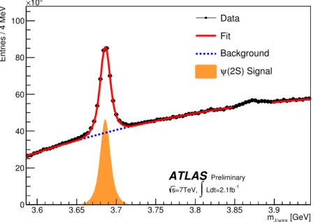
Figure 1 shows the
J/ψππinvariant mass distribution after the above selection cuts. A clear peak of the ψ(2S) is observed near 3.69 GeV. At larger invariant mass a further structure is also observed, identified as the
X(3872).[GeV]
π π ψ
mJ/
3.6 3.65 3.7 3.75 3.8 3.85 3.9
Entries / 4 MeV
0 20 40 60 80 100
103
×
Data Fit
Background (2S) Signal ψ
ATLAS Preliminary Ldt=2.1fb-1
∫
=7TeV, s
Figure 1: The uncorrected
J/ψππmass spectrum between 3.586 and 3.946 GeV. Superimposed on the data points is the result of a fit using a double Gaussian to describe the
J/ψππsignal peak, and a 2nd order Chebyshev polynomial to model the background, where the region within
±25 MeV of the X(3872)(m
J/ψππ =3.872 GeV) is excluded from the fit.
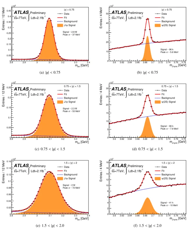
The cross-section measurements presented in this note are presented in three ψ(2S) rapidity intervals:
|y|
< 0.75, 0.75 <
|y|< 1.5, and 1.5 <
|y|< 2.0. Figure 2 illustrates the uncorrected yields and the resolutions of the di-muons (left) and the
J/ψ ππsystem (right) in the three rapidity regions, which comprise about 96,000, 66,000 and 41,000 ψ(2S) candidates respectively.
For both the di-muon and the
J/ψππinvariant mass fits, a double Gaussian is used to describe the signal shape, and a second-order Chebyshev polynomial to model the background. The two-dimensional distribution in
pTand
|y|of all
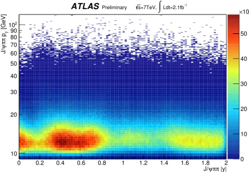
J/ψππcandidates contributing to Figure 2, is shown in Figure 3.
4 Cross-Section Determination
The differential production cross-section for ψ(2S) can be categorised into prompt production and non-
prompt production. The prompt ψ(2S) has no significant feed-down from higher mass charmonium
states, since they decay predominantly to
DD, so production proceeds directly via QCD production of a¯
charm-quark pair which subsequently binds to form the ψ(2S). Non-prompt ψ(2S) production processes
are distinguished from prompt processes by their longer apparent lifetimes, with production occurring
through the decay of a
b-hadron. Since in this analysis theb-hadron is not fully reconstructed, it is notpossible to use its lifetime to isolate prompt from non-prompt production. Instead, to distinguish between
these prompt and non-prompt processes, a parameter called pseudo-proper lifetime τ is constructed using
[GeV]
µ
mµ
2.8 2.9 3 3.1 3.2 3.3 3.4
Entries / 12 MeV
0 0.05 0.1 0.15 0.2 0.25 0.3 0.35 0.4 0.45
106
×
|y| < 0.75 Data Fit Background
Signal ψ J/
Signal ~ 2.8 M ~ 37 MeV σ Peak
ATLASPreliminary Ldt=2.1fb-1
∫
=7TeV, s
(a)|y|<0.75
[GeV]
π π ψ
mJ/
3.6 3.62 3.64 3.66 3.68 3.7 3.72 3.74 3.76 3.78
Entries / 4 MeV
0 10 20 30 40 50
103
×
|y| < 0.75 Data Fit Background
(2S) Signal ψ
Signal ~ 96 k ~ 5.6 MeV σ Peak
ATLAS Preliminary Ldt=2.1fb-1
∫
=7TeV, s
(b)|y|<0.75
[GeV]
µ
mµ
2.8 2.9 3 3.1 3.2 3.3 3.4
Entries / 12 MeV
0 0.05 0.1 0.15 0.2 0.25
106
×
0.75 < |y| < 1.5 Data Fit Background
Signal ψ J/
Signal ~ 2.3 M ~ 53 MeV σ Peak
ATLASPreliminary Ldt=2.1fb-1
∫
=7TeV, s
(c) 0.75<|y|<1.5
[GeV]
π π ψ
mJ/
3.6 3.62 3.64 3.66 3.68 3.7 3.72 3.74 3.76 3.78
Entries / 4 MeV
0 5 10 15 20 25 30
103
×
0.75 < |y| < 1.5 Data Fit Background
(2S) Signal ψ
Signal ~ 66 k ~ 7.9 MeV σ Peak
ATLAS Preliminary Ldt=2.1fb-1
∫
=7TeV, s
(d) 0.75<|y|<1.5
[GeV]
µ
mµ
2.8 2.9 3 3.1 3.2 3.3 3.4
Entries / 12 MeV
0 0.02 0.04 0.06 0.08 0.1 0.12 0.14 0.16
106
×
1.5 < |y| < 2 Data Fit Background
Signal ψ J/
Signal ~ 2 M ~ 72 MeV σ Peak
ATLASPreliminary Ldt=2.1fb-1
∫
=7TeV, s
(e) 1.5<|y|<2.0
[GeV]
π π J/ψ
m
3.6 3.62 3.64 3.66 3.68 3.7 3.72 3.74 3.76 3.78
Entries / 4 MeV
0 2 4 6 8 10 12 14 16 18
103
×
1.5 < |y| < 2 Data Fit Background
(2S) Signal ψ
Signal ~ 41 k ~ 10 MeV σ Peak
ATLAS Preliminary Ldt=2.1fb-1
∫
=7TeV, s
(f) 1.5<|y|<2.0
Figure 2: Uncorrected yields and the invariant mass resolutions for the di-muon (left) and
J/ψπ+π
−system (right) in the three rapidity ranges of the measurement. The data distributions are fitted with a
combination of two Gaussians (for the signal peak) and a second order polynomials (for backgrounds).
π |y|
π ψ J/
0 0.2 0.4 0.6 0.8 1 1.2 1.4 1.6 1.8 2
[GeV] T pππψJ/
10 20 30 40 50 60 70 80 90 102
0 10 20 30 40 50 103
ATLAS Preliminary s=7TeV,
∫
Ldt=2.1fb-1 ×Figure 3: Distribution of ψ(2S)
→ J/ψπ+π
−candidates in the mass interval 3.586 <
mJ/ψπ+π−<
3.786 GeV as a function of ψ(2S) transverse momentum and rapidity, before correction for e
fficiencies, acceptance, and detector resolution effects.
the
J/ψππtransverse momentum:
τ
= LxymJ/ψππpT
, (1)
with
Lxydefined by the equation:
Lxy≡
~
L·~
pT/p
T, (2)
where ~
Lis the vector from the primary vertex to the
J/ψππdecay vertex and ~
pTis the transverse mo- mentum vector of the
J/ψππ. The primary vertex is defined as the vertex with the largest associatedcharged-particle track
p2Tscalar sum, which we identify as the location of the primary proton-proton in- teraction. The presence of additional simultaneous proton-proton collisions, and the e
ffect of associating the final state particles to the wrong collision was found to have a negligible impact on the decay length determination or the signal extraction.
To obtain a measurement of the production cross-sections, the reconstructed candidates are first in- dividually weighted to correct for detector e
ffects, such as acceptance, muon reconstruction e
fficiency, pion reconstruction efficiency and trigger efficiency. The distribution of candidates in ψ(2S)
pTand
|y|
intervals are then fitted using a weighted two-dimensional unbinned maximum likelihood method, performed on the invariant mass and pseudo-proper lifetime distributions to isolate signal candidates from the backgrounds and separate prompt signal from non-prompt signal. The corrected prompt and non-prompt signal yields (N
Pψ(2S),
NNPψ(2S)) are then used to calculate the di
fferential cross-section times branching ratio, using the equation:
Br
ψ(2S)
→ J/ψ(→µ+µ
−)π
+π
−×
d
2σ
P/NP(ψ(2S))
d
pTdy = NP/NPψ(2S)∆pT∆
y
RLdt
, (3)
where
RLdt
is the total integrated luminosity,
∆pTand
∆y are the sizes of the intervals in ψ(2S) trans- verse momentum and rapidity, respectively, and
Brψ(2S)
→J/ψ(→µ+µ
−)π
+π
−is the total branching
ratio of the signal decay, taken to be 0.0202
±0.004, obtained by combining the world average values for
Br J/ψ→µ
+µ
−and
Brψ(2S)
→J/ψπ+π
−[15].
In addition to the prompt and non-prompt production cross-sections, the non-prompt ψ(2S) produc- tion fraction
fBψ(2S)is simultaneously extracted from the maximum likelihood fits to the same kinematic intervals. This fraction is defined as the corrected yield of non-prompt ψ(2S) divided by the corrected total yield of produced ψ(2S), as seen in the equation:
fBψ(2S) ≡ NNPψ(2S) NPψ(2S)+NNPψ(2S)
. (4)
Determination of this fraction has the advantage that many acceptance and efficiency effects cancel or are reduced in the ratio and so systematic uncertainties on this quantity are minimised.
Acceptance
The acceptance
A(pT, y,
mππ) is defined as the probability that the decay products in ψ(2S)
→ J/ψ(→µ
+µ
−)π
+π
−fall within the fiducial volume (
pT(µ
±) > 4 GeV,
|η(µ±)| < 2.3,
pT(π
±) > 0.5 GeV,
|η(π±)| <
2.5). It has been shown [16] that the final state is largely dominated by the simplest angular momentum configuration, where the two pions are in a relative
S-wave state, and the
J/ψand di-pion system are in
S-wave as well. Consequently, the spin-alignment state of the ψ(2S) is directly transferred to the
J/ψ. The acceptance depends on the spin-alignment ofψ(2S). For the central results obtained in this analysis, the ψ(2S) was assumed to be isotropic, with variations corresponding to a number of extreme spin-alignment scenarios detailed below, in Table 3.
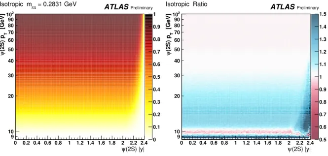
The acceptance maps are created using a high statistics generator-level Monte Carlo simulation, which randomly creates and decays ψ(2S)
→ J/ψ(→µ
+µ
−)π
+π
−, as a function of the ψ(2S) trans- verse momentum and rapidity, in finely-binned intervals of the di-pion invariant mass
mπ+π−covering the allowed range, 2m
π<
mπ+π−<
mψ(2S)−mJ/ψ. An example of the acceptance map for the lowest di-pion mass (m
π+π− =2m
π) is shown in Figure 4(a) for the isotropic ψ(2S) assumption. The variation of acceptance with di-pion mass is illustrated by the ratio of the acceptance at the lowest di-pion mass
mπ+π− =2m
πto the acceptance at the highest di-pion mass
mπ+π− =mψ(2S)−mJ/ψshown in Figure 4(b).
The largest variations are observed at low
pTand at high rapidity, where relative acceptance can vary by up to 50%.
The spin-alignment of
J/ψfrom ψ(2S) decay is, as mentioned above, assumed to be fully transferred from the spin-alignment of ψ(2S) and hence, in general, in its decay frame the angular dependence of the decay
J/ψ→µ
+µ
−is given by
d
2Nd cos θ
∗dφ
∗ ∝1 3
+λ
θ!
1
+λ
θcos
2θ
∗+λ
φsin
2θ
∗cos 2φ
∗+λ
θφsin 2θ
∗cos φ
∗, (5)
where the λ
iare coe
fficients related to the spin density matrix elements of the ψ(2S) wavefunction. Here, in the helicity frame, θ
∗is the angle between the momentum of the µ
+and the direction of the
J/ψmomentum in the lab frame, while φ
∗is the angle between the production and decay planes of the
J/ψ.In the default case of isotropic ψ(2S), all three λ
icoe
fficients in Eq. 5 are equal to zero. This assumption is compatible with recent measurements [17].
In certain areas of the phase space, the acceptance
Amay depend quite strongly on the values of the λ coe
fficients in Eq. 5 and we have identified seven extreme cases that lead to the largest possible variations of acceptance within the phase space of this measurement. These are used to define a range in which the results may vary under any physically-allowed spin-alignment assumptions:
•
isotropic distribution independent of θ
∗and φ
∗:
λ
θ =λ
φ=λ
θφ=0, Isotropic;
(2S) |y|
ψ 0 0.2 0.4 0.6 0.8 1 1.2 1.4 1.6 1.8 2 2.2 2.4 [GeV] T(2S) pψ
9 10 20 30 40 50 60 70 80 90 102
0 0.1 0.2 0.3 0.4 0.5 0.6 0.7 0.8 0.9 1 = 0.2831 GeV
π
Isotropic mπ ATLASPreliminary
(a) Lowest di-pion mass interval
(2S) |y|
ψ 0 0.2 0.4 0.6 0.8 1 1.2 1.4 1.6 1.8 2 2.2 2.4 [GeV] T(2S) pψ
9 10 20 30 40 50 60 70 80 90 102
0.5 0.6 0.7 0.8 0.9 1 1.1 1.2 1.3 1.4 1.5
Isotropic Ratio ATLASPreliminary
(b) Ratio of acceptances for lowest to highest di-pion masses
Figure 4: Example of ψ(2S)
→ J/ψ(→µ+µ
−)π
+π
−acceptance for (a) the lowest di-pion mass,
mπ+π− =2m
π, and (b) the acceptance ratio at lowest di-pion masses to the highest di-pion masses. The
J/ψ →µ
+µ
−decay is assumed to be isotropic.
•
longitudinal alignment:
λ
θ =−1, λφ=λ
θφ=0, Longitudinal;
•
three types of transverse alignment:
λ
θ = +1, λ
φ=λ
θφ=0, Transverse zero λ
θ = +1, λ
φ= +1, λ
θφ=0, Transverse positive λ
θ = +1, λφ=−1, λ
θφ=0, Transverse negative;
•
two types of o
ff-(λ
θ−λ
φ)-plane alignment:
λ
θ =0, λ
φ=0, λ
θφ= +0.5, Off-plane positiveλ
θ =0, λ
φ=0, λ
θφ=−0.5, Off-plane negative.
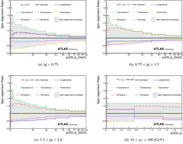
Figure 5 illustrates the variation of the acceptance correction weights with
pTand rapidity, for the six anisotropic spin-alignment scenarios described above, relative to the isotropic case.
Muon Reconstruction E ffi ciency
The muon reconstruction e
fficiency, determined using a data-driven tag-and-probe method [7] from
J/ψ→µ
+µ
−decays is given by:
recoµ =trk(
pµT1, η
µ1)
·trk(
pµT2, η
µ2)
·µ(
pµT1,
qµ1·η
µ1)
·µ(
pµT2,
qµ2·η
µ2), (6)
where
qis the charge of the muon,
trkis the muon track reconstruction e
fficiency in the ID, while
µis
the efficiency of the combined muon reconstruction given that the muon track has been reconstructed in
the ID. The muon track reconstruction efficiency
trkis determined [7] to be 99
±1% within the kinematic
range of interest.
[GeV]
(2S) pT
ψ
10 20 30 40 50 60 70 80 90 100
Spin-alignment Ratio
0.6 0.8 1 1.2 1.4 1.6 1.8 2
|y| < 0.75 Isotropic Longitudinal
Transverse 0 Transverse + Transverse -
Off-plane + Off-plane - Spin-alignment envelope
ATLASPreliminary
(a)|y|<0.75
[GeV]
(2S) pT
ψ
10 20 30 40 50 60 70 80 90 100
Spin-alignment Ratio
0.6 0.8 1 1.2 1.4 1.6 1.8 2
0.75 < |y| < 1.5 Isotropic Longitudinal
Transverse 0 Transverse + Transverse -
Off-plane + Off-plane - Spin-alignment envelope
ATLASPreliminary
(b) 0.75<|y|<1.5
[GeV]
(2S) pT
ψ
10 20 30 40 50 60 70 80 90 100
Spin-alignment Ratio
0.6 0.8 1 1.2 1.4 1.6 1.8 2
1.5 < |y| < 2.0 Isotropic Longitudinal
Transverse 0 Transverse + Transverse -
Off-plane + Off-plane - Spin-alignment envelope
ATLASPreliminary
(c) 1.5<|y|<2.0
(2S) |y|
ψ
0 0.2 0.4 0.6 0.8 1 1.2 1.4 1.6 1.8 2
Spin-alignment Ratio
0.6 0.8 1 1.2 1.4 1.6 1.8 2
< 100 GeV
10 < pT Isotropic Longitudinal
Transverse 0 Transverse + Transverse -
Off-plane + Off-plane - Spin-alignment envelope
ATLASPreliminary
(d) 10<pT <100 [GeV]
Figure 5: Average acceptance correction relative to the isotropic scenario for the seven extreme spin- alignment scenarios described in the text, as a function of ψ(2S) transverse momentum in the three rapidity regions (a)-(c), and versus ψ(2S ) rapidity for
pT> 10 GeV (d).
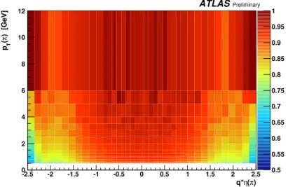
Pion Reconstruction E ffi ciency
The pion reconstruction e
fficiency
recoπis given by:
recoπ =π(p
πT1,
qπ1·η
π1)
·π(
pπT2,
qπ2·η
π2), (7)
where the two
πwere extracted from the map, shown in Figure 6, which was determined using tech-
niques derived for existing tracking efficiency measurements [18]. Pions produced in Monte Carlo event
simulation (fully simulated PYTHIA [19] sample of ψ(2S) production, using the ATLAS 2011 MC tun-
ing [20]) were used to determine the efficiencies in the interval
pT> 0.5 GeV and
|η|< 2.5. The pion
track reconstruction efficiencies are calculated in intervals of charge-signed pseudorapidity
q·η and track
transverse momentum
pTfrom Monte Carlo. In addition to the statistical uncertainties on the e
fficiency
due to limited Monte Carlo simulation, each efficiency value also contains an additional uncertainty to
account for any possible mis-modelling in the simulations.
) (π q*η
-2.5 -2 -1.5 -1 -0.5 0 0.5 1 1.5 2 2.5
) [GeV]π(Tp
0 2 4 6 8 10 12
0.5 0.55 0.6 0.65 0.7 0.75 0.8 0.85 0.9 0.95 1
ATLASPreliminary
Figure 6: Pion reconstruction e
fficiency map, as a function of pion charge-signed pseudorapidity and transverse momentum, obtained from simulation.
Trigger E ffi ciency
The trigger e
fficiency for the di-muon trigger used in this analysis has been measured in Ref. [7] from
J/ψ →µ
+µ
−and
Υ →µ
+µ
−decays using a data-driven method. The trigger e
fficiency is the e
fficiency for the trigger system to select signal events that also pass the reconstruction-level analysis selection, and is parameterised as:
trig=RoI(p
T1,
q1, η
1)
·RoI(p
T2,
q2, η
2)
·cµµ(∆
R,|yµµ|)(8) where
RoIis the efficiency of the trigger system to find a RoI for a single muon and
cµµis a correction term taking into account muon-muon correlations, dependent on the angular separation
∆Rbetween the two muons, and the absolute rapidity of the di-muon system,
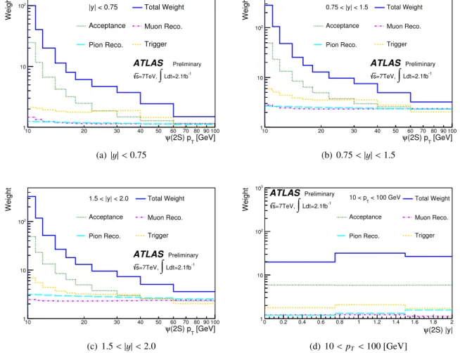
|yµµ|.Total Weight
The total weight w for each
J/ψππcandidate was calculated as the inverse of the product of acceptance and efficiency corrections, as described by:
w
−1=A(
pT, y,
mππ)
·recoµ ·recoπ ·trig. (9) The average of the total weight and its breakdown into components is illustrated in Figure 7, shown for the three rapidity regions for each
pTbin of the measurement, and also shown as an average over the full transverse momentum range (10 <
pT< 100 GeV) versus rapidity.
Fitting Procedure
A two-dimensional weighted unbinned maximum likelihood fit is performed on the
J/ψππinvariant mass
and pseudo-proper lifetime for each
pTand
|y|bin. The Probability Density Function (PDF) is defined
as a normalised sum of terms, where each term was factorized into a mass-dependent and lifetime-
dependent function. The PDF can be written in a compact form as:
[GeV]
(2S) pT
10 20 30 40 50 ψ60 70 80 90 100
Weight
1 10
102 |y| < 0.75 Total Weight
Acceptance Muon Reco.
Pion Reco. Trigger ATLAS Preliminary
Ldt=2.1fb-1
∫
=7TeV, s
(a)|y|<0.75
[GeV]
(2S) pT
10 20 30 40 50ψ60 70 80 90 100
Weight
1 10 102
0.75 < |y| < 1.5 Total Weight
Acceptance Muon Reco.
Pion Reco. Trigger
ATLAS Preliminary Ldt=2.1fb-1
∫
=7TeV, s
(b) 0.75<|y|<1.5
[GeV]
(2S) pT
10 20 30 40 50 ψ60 70 80 90 100
Weight
1 10 102
1.5 < |y| < 2.0 Total Weight
Acceptance Muon Reco.
Pion Reco. Trigger
ATLAS Preliminary Ldt=2.1fb-1
∫
=7TeV, s
(c) 1.5<|y|<2.0
(2S) |y|
ψ
0 0.2 0.4 0.6 0.8 1 1.2 1.4 1.6 1.8 2
Weight
1 10 102 103
< 100 GeV
10 < pT Total Weight
Acceptance Muon Reco.
Pion Reco. Trigger
ATLAS Preliminary Ldt=2.1fb-1
∫
=7TeV, s
(d) 10<pT <100 [GeV]
Figure 7: Average correction weights for the three rapidity regions versus
pT(a)-(c) and for the full
pTregion versus
|y|(d).
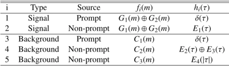
PDF(m, τ)
= X5i=1
⊕fi
(m)
·hi(τ)
⊗G(τ).(10) Here the symbol
⊕stands for a normalised sum of various terms, while
⊗denotes a convolution between two functions. The functions
fiand
hifor the mass and lifetime components of the sum,
i=1, . . . , 5 are shown in Table 1, where
Gk,
Ck, and
Ekstand for Gaussians, second order Chebyshev polynomials and exponential functions, respectively, and the index
kcorresponds to different sets of parameters, while δ stands for the Dirac delta function. The lifetime resolution function,
G(τ), is assumed to be Gaussian,Table 1: Components of the probability density function.
i Type Source
fi(m)
hi(τ)
1 Signal Prompt
G1(m)
⊕G2(m) δ(τ)
2 Signal Non-prompt
G1(m)
⊕G2(m)
E1(τ)
3 Background Prompt
C1(m) δ(τ)
4 Background Non-prompt
C2(m)
E2(τ)
⊕E3(τ) 5 Background Non-prompt
C3(m)
E4(
|τ|)
with a mean fixed to zero and a width that is free to be determined from each of the fits.
The two signal Gaussians
G1and
G2are required to have a common mean, while the respective widths σ
1,2are required to satisfy the relation σ
2 =1.5
·σ
1, so
G2is always fitted to the wider part of the signal peak (the factor of 1.5 was determined from test fits). To constrain the fit model better at high
pT, the widths (σ
1) of the mass signal Gaussians (for prompt and non-prompt) are obtained for each bin from separate fits to the invariant mass distributions, using the same
fi(m) terms. The resultant fitted σ values of the one-dimensional fits are parameterised as a linear function of
pTfor each of the three rapidity regions, and used to fix the widths in each of the two-dimensional fits. Figure 8 illustrates the results of the unbinned maximum likelihood fits to the data for three representative kinematic intervals.
5 Systematic Uncertainties
Various sources of systematic uncertainties on the measurement are considered and are outlined below.
Acceptance Corrections
The acceptance maps were generated using high statistics Monte Carlo simulation, with negligible sta- tistical and systematic uncertainties.
Fit Model Variations
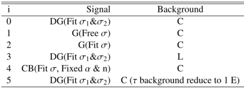
The uncertainty on the fit was determined by changing one component at a time of the fit model described
in Section 4, creating a set of new fit models. For each new fit model the cross-section was recalculated,
and in each
pTand
|y|interval the maximal variation from the central fit model was used as its systematic
uncertainty. The full set of fit models used are documented in Table 2. The central fit model is the
double Gaussian mass signal and second order Chebyshev polynomial for mass background (Model 0
in Table 2), where G, C and E are the same as defined in Section 4. DG is a double Gaussian, CB is a
crystal ball function [21], with the α and
nparameters fixed to 2 (determined from test fits), L is a linear
[GeV]
π π ψ
mJ/
3.6 3.62 3.64 3.66 3.68 3.7 3.72 3.74 3.76 3.78
Entries / 4 MeV
0 0.02 0.04 0.06 0.08 0.1 0.12 0.14 0.16 0.18 106
× Data Fit Background Prompt Signal Non Prompt Signal
ATLASPreliminary Ldt=2.1fb-1
∫
=7TeV, s
[ps]
π π ψ
τJ/
-2 0 2 4 6 8 10
Entries / 0.12 ps
1 10 102 103 104 105
106 Data
Fit Prompt Signal Prompt Background Non Prompt Signal Non Prompt Background
ATLASPreliminary Ldt=2.1fb-1
∫
=7TeV, s
(a) |y|<0.75, 11<pT<12 GeV
[GeV]
π π ψ
mJ/
3.6 3.62 3.64 3.66 3.68 3.7 3.72 3.74 3.76 3.78
Entries / 4 MeV
0 5 10 15 20 25 30 35 103
× Data Fit Background Prompt Signal Non Prompt Signal
ATLASPreliminary Ldt=2.1fb-1
∫
=7TeV, s
[ps]
π π J/ψ
-2 0 2 4 6 8τ 10
Entries / 0.12 ps
1 10 102 103 104 105
Data Fit Prompt Signal Prompt Background Non Prompt Signal Non Prompt Background
ATLASPreliminary Ldt=2.1fb-1
∫
=7TeV, s
(b) 0.75<|y|<1.5, 16<pT<18 GeV
[GeV]
π π ψ
mJ/
3.6 3.62 3.64 3.66 3.68 3.7 3.72 3.74 3.76 3.78
Entries / 4 MeV
0 50 100 150 200 250 300 350
Data Fit Background Prompt Signal Non Prompt Signal
ATLASPreliminary Ldt=2.1fb-1
∫
=7TeV, s
[ps]
π π ψ
τJ/
-2 0 2 4 6 8 10
Entries / 0.12 ps
1 10 102 103
Data Fit Prompt Signal Prompt Background Non Prompt Signal Non Prompt Background
ATLASPreliminary Ldt=2.1fb-1
∫
=7TeV, s
(c) 1.5<|y|<2.0, 40<pT<60 GeV
Figure 8: Unbinned maximum likelihood fit and data projections onto the invariant mass and pseudo-
proper lifetimes of the ψ(2S) candidates for three representative kinematic intervals studied in this
measurement. Total signal plus background fits to the data are shown, along with the breakdown by
prompt/non-prompt production for the ψ(2S) signal.
Table 2: Fit models used to test sensitivity of extracted ψ(2S) yields to the signal and background mod- elling. The symbols are described in the text.
i Signal Background
0 DG(Fit σ
1&σ
2) C
1 G(Free σ) C
2 G(Fit σ) C
3 DG(Fit σ
1&σ
2) L
4 CB(Fit σ, Fixed α & n) C
5 DG(Fit σ
1&σ
2) C (τ background reduce to 1 E)
Chebyshev polynomial, Fit σ is the result of the fitted σ (defined in Section 4) and Free σ is when the σ is completely free. For all these models the lifetime component was varied by modifying the exponential terms for the background.
ID Tracking E ffi ciency for Muons
The ID tracking e
fficiency for muon tracks varies as a function of track transverse momentum and pseu- dorapidity in the kinematic intervals studied in this note. The tracking efficiency also has a small de- pendence on the number of simultaneous proton-proton collisions that occur in the event in question.
These variations are contained within a band of
±1% from the nominal value of 99% determined for theefficiency, and this band is directly assigned as a systematic uncertainty on measured the cross-sections.
Muon Reconstruction and Trigger E ffi ciencies
Uncertainties on the muon reconstruction and muon trigger efficiencies arise predominantly from sta- tistical uncertainties due to the finite size of the data samples used to determine the e
fficiencies. The uncertainties on the ψ(2S) yields are determined by randomly and independently (bin to bin) varying the values of these efficiencies within their uncertainties and recalculating the weights used to extract cross-sections. A Gaussian fit to the distribution of the average weight from many trials is used to extract the width of the weight distribution, which is assigned as the systematic uncertainty on the cross-section due to efficiency uncertainties.
Pion Track Reconstruction E ffi ciency
The pion track reconstruction uncertainty contains the contributions from statistical uncertainties in the pion e
fficiency maps, which are estimated using the same procedure as for the muon e
fficiency maps.
With the addition of uncertainties that are due to the data simulation, these are estimated to be 2%
−3%
per pion in the
pTranges considered, varying with rapidity; and an additional 1% contribution per pion for the hadronic interaction uncertainties.
Selection Criteria
For the constrained
J/ψπ+π
−fit quality cut, the e
fficiency was measured to vary between 93% and 97% as a function of
pT, with an uncertainty of about 2% estimated from the bin-to-bin variation of the efficiency.
Other selection ine
fficiencies and their corresponding uncertainties were estimated using simulations to
be at or below the 1% level. The systematic error on the selection e
fficiency was obtained by summing
in quadrature all uncertainties.
Luminosity
The uncertainty on the integrated luminosity for the dataset studied in this note has been determined [13]
to be 1.8%. This systematic uncertainty does not apply to the measurement of the non-prompt production fraction.
Total Uncertainties
Figures 9–11 summarise the total systematic and statistical uncertainties on the measurement of the non- prompt production fraction and the prompt/non-prompt cross-sections.
[GeV]
(2S) pT
ψ
10 20 30 40 50 60 70 80 100
Fractional Uncertainty [%]
-30 -20 -10 0 10 20
30 ATLASPreliminary s=7TeV,
∫
Ldt=2.1fb-1Non-prompt fraction |y| < 0.75
Total Uncertainty
Total Systematics Statistical
Muon Reconstruction Pion Reconstruction Trigger
Inner Detector tracking Fit Model
Selection Criteria
[GeV]
(2S) pT
10 20 30 40 50 60 70 80ψ 102
Fractional Uncertainty [%]
-30 -20 -10 0 10 20
30 ATLASPreliminary s=7TeV,
∫
Ldt=2.1fb-1 Non-prompt fraction 0.75 < |y| < 1.5[GeV]
(2S) pT
ψ
10 20 30 40 50 60 70 80 100
Fractional Uncertainty [%]
-30 -20 -10 0 10 20
30 ATLASPreliminary s=7TeV,
∫
Ldt=2.1fb-1 Non-prompt fraction 1.5 < |y| < 2.0Figure 9: Summary of the positive and negative uncertainties for the non-prompt fraction measurement.
This plot does not include the spin-alignment uncertainty.
[GeV]
(2S) pT
ψ
10 20 30 40 50 60 70 80 100
Fractional Uncertainty [%]
-60 -40 -20 0 20 40 60
ATLASPreliminary s=7TeV,
∫
Ldt=2.1fb-1 Prompt - |y| < 0.75Total Uncertainty Total Systematics Statistical
Muon Reconstruction Pion Reconstruction Trigger
Inner Detector tracking Fit Model
Selection Criteria
[GeV]
(2S) pT
ψ
10 20 30 40 50 60 70 80 100
Fractional Uncertainty [%]
-60 -40 -20 0 20 40 60
ATLASPreliminary s=7TeV,
∫
Ldt=2.1fb-1 Prompt - 0.75 < |y| < 1.5[GeV]
(2S) pT
ψ
10 20 30 40 50 60 70 80 100
Fractional Uncertainty [%]
-60 -40 -20 0 20 40 60
ATLASPreliminary s=7TeV,
∫
Ldt=2.1fb-1 Prompt - 1.5 < |y| < 2.0Figure 10: Summary of the positive and negative uncertainties for the prompt cross-section measurement.
This plot does not include the constant 1.8% luminosity uncertainty or the spin-alignment uncertainty.
[GeV]
(2S) pT
ψ
10 20 30 40 50 60 70 80 100
Fractional Uncertainty [%]
-60 -40 -20 0 20 40 60
ATLASPreliminary s=7TeV,
∫
Ldt=2.1fb-1 Non-prompt - |y| < 0.75Total Uncertainty Total Systematics Statistical
Muon Reconstruction Pion Reconstruction Trigger
Inner Detector tracking Fit Model
Selection Criteria
[GeV]
(2S) pT
10 20 30 40 50 60 70 80ψ 102
Fractional Uncertainty [%]
-60 -40 -20 0 20 40 60
ATLASPreliminary s=7TeV,
∫
Ldt=2.1fb-1 Non-prompt - 0.75 < |y| < 1.5[GeV]
(2S) pT
ψ
10 20 30 40 50 60 70 80 100
Fractional Uncertainty [%]
-60 -40 -20 0 20 40 60
ATLASPreliminary s=7TeV,