ATLAS NOTE ATLAS-CONF-2015-058

ATLAS-CONF-2015-058 09/12/2015

ATLAS NOTE

ATLAS-CONF-2015-058

26th November 2015 Minor revision: 9th December 2015

Study of hard double parton scattering in four-jet events in p p collisions at √

s = 7 TeV with the ATLAS experiment at the LHC

The ATLAS Collaboration

Abstract

Inclusive four-jet events produced in proton–proton collisions at a center-of-mass energy of

√ s = 7 TeV have been analysed for the presence of hard double parton scattering using data corresponding to an integrated luminosity of ( 37 . 3 ± 1 . 3 ) pb

, collected with the ATLAS detector at the LHC. The contribution of hard double parton scattering to the production of four-jet events has been extracted using an artificial neural network. The assumption was made that hard double parton scattering can be represented by a random combination of dijet events. The fraction of events that corresponds to the contribution made by hard double parton scattering was estimated to be f

= 0 . 084

(stat.)

0.036

(syst.) in four-jet events, where each event contains at least four jets with transverse momentum, p

≥ 20 GeV, pseudo-rapidity, |η | ≤ 4 . 4, and the highest- p

jet has p

≥ 42 . 5 GeV. After combining this measurement with those of the dijet and four-jet cross-sections in the appropriate phase- space regions, the effective overlap area between the interacting protons, σ

, was found to be σ

= 16 . 1

(stat.)

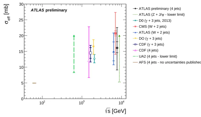
(syst.) mb. This result is consistent within the quoted uncer- tainties with previous measurements of σ

, performed at center-of-mass energies between 63 GeV and 8 TeV using various final states, and it corresponds to ( 20 ± 10 ) % of the total inelastic cross-section measured at

√ s = 7 TeV.

December 9, 2015: Modified legend of Figure 7.

© 2015 CERN for the benefit of the ATLAS Collaboration.

Reproduction of this article or parts of it is allowed as specified in the CC-BY-3.0 license.

1 Introduction

Interactions with more than one pair of incident partons in the same hadronic collision have been dis- cussed on theoretical grounds since the introduction of the parton model to the description of particle production in collisions with hadronic initial states [1–3]. These first studies were readily followed by the generalization of the Altarelli–Parisi evolution equations to the case of multi-parton states in [4, 5] or with other considerations concerning possible correlations in the color and spin degrees of freedom of the incident partons [6]. In a first wave of phenomenological studies of such effects, the most prominent role has been played by processes known as double parton scattering (DPS), which is the simplest case of multi-parton interactions, leading to final states such as four leptons, four jets, three jets plus a photon, or a leptonically decaying gauge boson accompanied by two jets [7–15]. These studies have been sup- plemented by experimental measurements of DPS effects in hadron collisions at different center-of-mass energies, which now range over two orders of magnitude from 63 GeV to 8 TeV [16–25] and which firmly establish the existence and impact of this mechanism. Recent and forthcoming measurements of multi-parton scattering processes at the LHC have re-ignited the phenomenological interest in DPS and have led to a deepening of its theoretical understanding [26–34]. However, despite this theoretical progress, quantitative measurements of the impact of DPS on distributions of sensitive observables have large statistical and systematic uncertainties. This is a clear indication of the experimental challenges and of the complexity of the analysis related to such measurements. Therefore, the cross-section of DPS is still estimated by ignoring complicated, but probably real, correlation effects. For a process in which a final state A + B is being produced at a hadronic center-of-mass energy

√ s , the simplified formalism of [12, 13]

yields

d ˆ σ

(s) = 1 1 + δ

d ˆ σ

(s) d ˆ σ

( s)

σ

( s) . (1)

The quantity δ

is the Kronecker delta used to construct a symmetry factor such that for identical final states with identical phase space, the DPS cross-section is divided by two. The σ

is a purely phenomenological parameter determining the overall size of DPS cross-sections. At values typical for hadronic cross-sections, it has been measured to range between 10 and 20 mb. In the equation above, the various ˆ σ are the parton-level cross-sections, either for the DPS events, indicated by the superscript, or for the production of a final state A or B in a single parton scatter (SPS), given by

d ˆ σ

( s) = 1 2 s

X

i j

Z

d x

f

( x

, µ

) d x

f

( x

, µ

)d Φ

|M

( x

x

s, µ

, µ

)|

. (2)

Here the functions f

(x, µ

) are the single parton distribution functions (PDFs) which at leading order parameterize the probability of finding a parton i at a momentum fraction x and a factorization scale µ

in the incident hadron, d Φ

is the invariant differential phase space element for the final state A, M is the perturbative matrix element for the process i j → A, and µ

is the renormalization scale at which the couplings are evaluated. To constrain the phase space to that allowed by the energy of each incoming proton, a simple two-parton PDF is defined as

f

( b, x

, x

, µ

) = Γ ( b) f

( x

, µ

) f

( x

, µ

) Θ ( 1 − x

− x

) , (3)

where Θ (x ) is the Heaviside step function, Γ ( b) the area overlap function, and the x and scale dependence

of the PDF is assumed to be independent of the impact-parameter b . Equation (3) reflects the omission of

correlations between the partons in the proton.

In this note, four-jet events are considered in phase space regions that are most sensitive to DPS. In one of the first studies of DPS in four-jet production at hadron colliders [10], the kinematic configuration in which there is a pair-wise balance of the transverse momenta ( p

) of the jets has already been identified as increasing the contribution of the DPS mechanism relative to the perturbative QCD production of four jets in SPS. The idea is that in typical 2 → 2 scattering processes the two outgoing particles – here the partons identified with jets later on – are oriented back-to-back in transverse space such that their net transverse momentum exactly cancels. Corrections to this simple picture are expected from initial and final state radiation as well as fragmentation and hadronization. In addition, the further possible parton interactions of the underlying event will add four-momentum to the overall configuration. Monte Carlo (MC) event generators form an integral part of any study, in order to establish a link between the experimentally observed four jets and the simple partonic picture of DPS described above as two almost independent 2 → 2 scatters.

1.1 Effective cross-section

After integrating the differential cross-sections in Eq. (1) over the phase-space defined by the selection requirements of the A and B final-states, the expression for the DPS cross-section in the four-jet final state is written as

σ

= 1

1 + δ

σ

2j

σ

2j

σ

, (4)

where σ

2j

( σ

2j

) is the measured cross-section for dijet events in the phase-space region labeled A (B). The assumed dependence of the cross-sections and σ

on s was dropped for simplicity. The four-jet (dijet) final state is defined inclusively [35, 36], such that at least four jets (two jets) are required in the event, while no restrictions are applied to additional jets. When measuring the cross-section of four-jet (dijet) events, the leading (highest- p

) four (two) jets in the event are considered.

The double parton scattering cross-section may be expressed as

σ

= f

· σ

, (5)

where σ

is the measured cross-section for four-jet events in the phase-space A + B, including all four-jet final states, namely both the SPS and DPS topologies, and where f

represents the fraction of DPS events in these four-jet final states. The main challenge of the measurement is the extraction of f

from optimally selected measured observables.

The DPS model contributes in two ways to the production of events with at least four jets, leading to two separate event classifications. In one contribution, the secondary scatter produces two of the four leading jets in the event; such events are classified as complete-DPS (cDPS). In the second contribution of DPS to four-jet production, three of the four leading jets are produced in the hardest scatter, and one jet is produced in the secondary scatter; such events are classified as semi-DPS (sDPS). The fraction f

is therefore re-written as f

+ f

and f

and f

are both determined from data. The dijet cross-sections in Eq. (4) do not require any modification since they are all inclusive cross-sections, i.e., the three-jet cross-section accounting for the production of a sDPS event is already included in the dijet cross-sections.

The general expression for the measured dijet and four-jet cross-sections may be written as σ

= N

C

L

, (6)

where the subscript nj denotes either dijet (2j) or four-jet (4j) topologies. For each nj channel, N

is the number of observed events, C

is the correction for detector effects, particularly due to the jet energy scale and resolution, and L

is the corresponding luminosity. Combining Eqs. (4) and (5) and defining

S

= N

/L

(7)

as the observed cross-section at the detector-level and α

2j

= C

C

2j

C

2j

, (8)

the expression from which σ

is determined can be written as σ

= 1

1 + δ

α

2j

f

+ f

S

2j

S

2j

S

. (9)

2 The ATLAS Detector

The ATLAS detector is described in detail in Ref. [37]. In this analysis, the tracking detectors are used to define candidate collision events by constructing vertices from tracks, and the calorimeters are used to reconstruct jets.

The inner detector used for tracking and particle identification has complete azimuthal coverage and spans the pseudo-rapidity region |η | < 2 . 5.1 It consists of layers of silicon pixel detectors, silicon microstrip detectors, and transition radiation tracking detectors, surrounded by a solenoid magnet that provides a uniform axial field of 2 T.

The electromagnetic calorimetry is provided by the liquid argon (LAr) calorimeters that are split into three regions: the barrel ( |η | < 1 . 475), the endcap (1 . 375 < |η| < 3 . 2) and the forward (FCal: 3 . 1 < |η | < 4 . 9) regions. The hadronic calorimeter is divided into four distinct regions: the barrel ( |η | < 0 . 8), the extended barrel (0 . 8 < |η | < 1 . 7), both of which are scintillator/steel sampling calorimeters, the hadronic endcap (HEC; 1 . 5 < |η | < 3 . 2), which has LAr/Cu calorimeter modules, and the hadronic FCal (same η -range as for the EM-FCal) which uses LAr/W modules. The total calorimeter coverage is |η | < 4 . 9.

The trigger system for the ATLAS detector consists of a hardware-based Level 1 (L1) and of a software- based higher-level trigger (HLT) [38]. Jets are first identified at L1 using a sliding window algorithm from coarse granularity calorimeter towers. This is refined using jets reconstructed from calorimeter cells in the HLT. Three different triggers are used to select events for this measurement: the minimum bias trigger scintillators, the central ( |η | < 3 . 2) and the forward jet triggers (3 . 1 < |η | < 4 . 9).

1ATLAS uses a right-handed coordinate system with its origin at the nominal interaction point (IP) in the center of the detector and thez-axis along the beam pipe. Thex-axis points from the IP to the center of the LHC ring, and theyaxis points upward.

Cylindrical coordinates(r, φ)are used in the transverse plane,φbeing the azimuthal angle around the beam pipe, referred to the x-axis. The pseudo-rapidity is defined in terms of the polar angleθwith respect to the beamline asη =−ln tan(θ/2). When dealing with massive jets and particles, the rapidityy= ¹₂ln

_E+pz

E−pz

is used, whereEis the jet energy andpzis the z-component of the jet momentum.

3 Monte Carlo simulation

Multi-jet events were generated using fixed order matrix elements (2 → n , with n = 2 , 3 , . . . , 6) with Alpgen 2.14 [39] utilizing the CTEQ6L1 PDF set [40], interfaced to Jimmy [41] and Herwig 6.520 [42]

using the AUET2 [43] set of parameters (tune). The MPI parameters in the AUET2 tune were optimised using early ATLAS data. The MLM [44] matching scale, the energy scale at which matching of matrix elements to parton showers begins, was set to 15 GeV. The implication of this choice is that partons with p

≥ 15 GeV in the final state, originate from matrix elements, and not from the parton shower.

Event record information is used to extract the SPS sample from the Alpgen + Herwig + Jimmy MC combination (AHJ). A sample of DPS events is also extracted from AHJ in order to study their topology and validate the measurement methodology.

Tree-level matrix-elements with up to six outgoing partons were used to generate a sample of multi-jet events within Sherpa 1.4.2 [45, 46] with the CT10 PDF set [47] and the default Sherpa tune. The CKKW [48, 49] matching scale was set to 15 GeV, similarly to the AHJ sample described above. Events were generated without multi-parton interactions by setting the internal flag, MI_HANDLER=None . This SPS sample is compared to the SPS sample extracted from the AHJ sample for validation purposes.

A sample of multi-jet events was generated with Pythia 6.425 [50] using a 2 → 2 matrix element at leading order with additional radiation modelled in the leading-logarithmic approximation by p

-ordered parton showers. The sample was generated utilizing the modified leading-order PDF set MRST LO* [51]

with the AMBT1 [52] set of parameters, tuned to describe the distributions measured by ATLAS in minimum bias collisions. The correction for detector effects is calculated using this sample.

Minimum-bias events generated with Pythia 6.423 using the MRST LO* PDF set with the AMBT1 tune are overlaid with the multi-jet events in order to account for the effects of multiple proton–proton interactions. Four-vectors of particles with a lifetime longer than 10 ps in the events generated are passed through the full ATLAS detector simulation. The Geant software toolkit [53] within the ATLAS simulation framework [54] propagates the particles through the ATLAS detector and simulates their interactions with the detector material. The energy deposited by particles in the active detector material is converted into detector signals with the same format as the ATLAS detector read-out. The simulated detector signals are in turn reconstructed with the same reconstruction software as used for the data.

Finally, simulated events are reconstructed and jets are calibrated in the same manner as in the data.

4 Cross-section measurements

4.1 Dataset and event selection

The measurement presented here is based on the full ATLAS 2010 data sample from proton–proton collisions at

√ s = 7 TeV. The trigger strategy used in this analysis is equivalent to that developed and used for the measurement of the dijet cross-section using 2010 data [55]. In total, data corresponding to a luminosity of ( 37 . 3 ± 1 . 3 ) pb

are used, where the systematic uncertainty on the integrated luminosity for 2010 proton–proton data is 3.5% [56].

To reject events initiated by cosmic-ray muons and other non-collision backgrounds, events are required to have at least one primary vertex, defined as a vertex that is consistent with the beam spot and which has at least five tracks with transverse momentum p

T

> 150 MeV associated with it. The primary vertex

associated with the event of interest is the one with the highest associated transverse track momentum P

p

T

. The efficiency for collision events to pass these requirements is well over 99%, while the contribution from fake vertices is negligible [55, 57].

In order to avoid the effects of multiple proton–proton interactions within the same bunch crossing (pile-up), the 2010 data set was chosen for this analysis because it had a low average number of proton–

proton interactions per bunch crossing of approximately 0.4. It was therefore possible to collect multi-jet events with low p

thresholds and to select with high efficiency for the analysis events with exactly one reconstructed primary vertex (single-vertex events), thereby removing any contribution from pile-up jets to the four-jet final state topologies.

Jets are identified using the anti- k

jet algorithm [58], implemented in the FASTJET [59] package, with a value R = 0 . 6, where R is the distance parameter. Two types of jets are used, particle jets and reconstructed jets. Particle jets are built from particles with a lifetime longer than 10 ps in the Monte Carlo event record, excluding muons and neutrinos. The inputs to reconstructed jets are three-dimensional topological clusters [60, 61] built from calorimeter cells, calibrated at the electromagnetic (EM) scale.2 A jet energy calibration is subsequently applied at the jet-level, relating the jet energy measured with the ATLAS calorimeter to the true energy of the corresponding jet of stable particles entering the detector. A full description of the jet energy calibration is given in Ref. [57].

For the purpose of measuring σ

in the four-jet final state, three samples of events are selected, two dijet samples and one four-jet sample. The former have at least two jets in the final state and the latter has at least four. Jets are required to have p

≥ 20 GeV and |η | ≤ 4 . 4. In each event, jets are sorted in decreasing order of their transverse momenta. Denoting p

T

the transverse momentum of the i

jet in an event, the jet with the highest- p

, p

T

, is referred to as the leading jet. The leading jet in four-jet events is required to have p

T

≥ 42 . 5 GeV to comply with the requirements of the low- p

jet triggers.

The selection requirements for the dijet samples are dictated by the requirements used to select four-jet events. In one class of dijet events, the requirement on the transverse momentum of the leading jet must be equivalent to the requirement on the leading jet in four-jet events, p

T

≥ 42 . 5 GeV. The other type of dijet events corresponds to the sub-leading pair of jets in the four-jet event, with a requirement p

≥ 20 GeV. In the following, the cross-section for dijets selected with p

≥ 20 GeV is denoted by σ

2j

and the cross-section for dijets with p

T

≥ 42 . 5 GeV is denoted by σ

2j

.

To summarize, the measurement is performed using the dijet A sample and its two sub-samples (dijet B and four-jet), selected using the following requirements:

(dijet A) N

≥ 2 , p

T

≥ 20 GeV , |η

| ≤ 4 . 4 , ( dijet B ) N

≥ 2 , p

T

≥ 42 . 5 GeV , p

T

≥ 20 GeV , |η

| ≤ 4 . 4 , (four-jet) N

≥ 4 , p

T

≥ 42 . 5 GeV , p

T

≥ 20 GeV , |η

| ≤ 4 . 4 ,

(10)

where N

is the number of reconstructed anti- k

, R = 0 . 6, jets in the event. All of the events considered in this study are corrected for jet reconstruction and trigger inefficiencies. The corrections range from 2%–4% for low p

jets and are less than 1% for jets with p

≥ 60 GeV. The observed distributions of the p

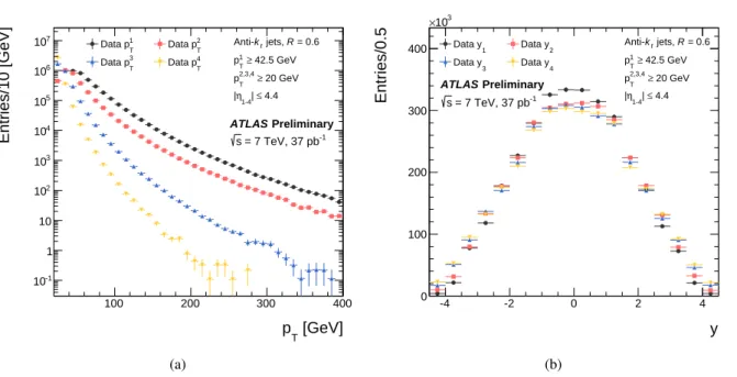
and y of the four leading jets in the selected events are shown in Figs. 1(a) and 1(b).

2The electromagnetic scale is the basic calorimeter signal scale to which the ATLAS calorimeters are calibrated. It has been established using test-beam measurements for electrons and muons to give the correct response for the energy deposited by electromagnetic showers, while it does not correct for the lower hadron response.

[GeV]

pT

100 200 300 400

Entries/10 [GeV]

10-1

1 10 102

103

104

105

106

107

Preliminary ATLAS

= 7 TeV, 37 pb-1

s

1

Data pT ²

Data pT 3

Data pT ⁴

Data pT

= 0.6 R jets, kt Anti-

42.5 GeV

≥ 1 pT

20 GeV

≥ 2,3,4 pT

≤ 4.4 1-4| η

|

(a)

y

-4 -2 0 2 4

Entries/0.5

0 100 200 300 400

103

×

Preliminary ATLAS

= 7 TeV, 37 pb-1

s Data y1

Data y2 Data y3

Data y4

= 0.6 R jets, kt Anti-

42.5 GeV

≥ 1 pT

20 GeV

≥ 2,3,4 pT

≤ 4.4 1-4| η

|

(b)

Figure 1: Distributions of the(a)transverse momentum,p_T, and(b)rapidity,y, of the four highest-p_Tjets, denoted asp¹⁻⁴

T andy₁−4in the figures, in four-jet events in data, selected in the phase-space defined in the figure.

4.2 Correction for detector effects

The correction for detector effects for each class of events is individually estimated using the Pythia6 MC sample. The same restrictions on the phase-space of reconstructed jets, defined in Eq. (10), are applied on particle jets. The correction is given by

C

nj

= N

N

nj

, (11)

where N

( N

nj

) is the number of n -jet events passing the (A or B) selection requirements using reconstructed (particle) jets.

The correction is sensitive to the migration of events into and out of the phase-space of the measurement.

Due to the very steep jet p

spectrum in dijet and four-jet events, it is crucial to have a good agreement between the jet p

spectra in data and MC close to the selection threshold before calculating the correction.

Therefore, the jet p

threshold was lowered to 10 GeV and the fiducial |η | range was increased to 4.5, and the events in the MC are re-weighted such that the jet p

- y distributions in data are reproduced by the MC. The value of α

2j

(see Eq. (8)), as determined from the re-weighted MC, is α

2j

= 0 . 94 ± 0 . 01 (stat.) ± 0 . 02 (syst.) , (12) where the first uncertainty is statistical and the second uncertainty is systematic. The systematic uncertainty arising from model-dependence is determined from a comparison with an alternate re-weighting method and from deriving α

2j

using Sherpa. Other systematic uncertainties are discussed in Section 6.

5 Determination of the fraction of DPS events

The main challenge in the measurement of σ

is to estimate the DPS contribution to the four-jet data sample. It is impossible to extract complete-DPS and semi-DPS candidate events on an event by event basis. Therefore, the usual approach is to fit the distributions of variables sensitive to cDPS and sDPS in the data to a combination of expected templates for the SPS, cDPS and sDPS contributions. The templates for SPS and sDPS contributions are extracted from the AHJ MC sample, while the cDPS template is obtained by overlaying two dijet events from the data. The analysis assumes that the SPS and sDPS templates from AHJ render properly the expected topologies, and no further attempt is made to quantify possible theoretical uncertainties associated with this assumption. For the SPS template, this assumption is supported by the good agreement observed between various distributions in the SPS samples in AHJ and in Sherpa. To exploit the full spectrum of variables sensitive to the various contributions and their correlations, an artificial neural network (NN) is used for the classification [62].

5.1 Template samples

In events generated in AHJ, the outgoing partons can be assigned to the primary interaction from the Alpgen ME generator or to a secondary interaction, generated by Jimmy, based on the event record. The former are referred to as primary-scatter partons and the latter are referred to as secondary-scatter partons.

The p

of secondary-scatter partons is required to be p

T

≥ 15 GeV , (13)

in order to match the minimum p

of primary-scatter partons which is set by the matching scale between radiation generated as part of the ME and radiation generated as part of the parton shower in AHJ. Once the outgoing partons are classified, the jets in the event are matched to outgoing partons and the event is classified as a SPS, cDPS or sDPS event.

The matching of jets to partons is done in the φ − y plane by calculating the angular distance between the jet and the outgoing parton as

∆R

= q

(y

− y

)

+ (φ

− φ

)

. (14) For 99% of the primary-scatter partons, the parton is within the distance ∆R

≤ 1 . 0, which is therefore used as a requirement for the matching of jets and partons.

Events in which none of the leading four jets are matched to a secondary-scatter parton are selected for the SPS sample. All of the soft MPI and underlying activity is therefore retained in the selected SPS events.

In the simple picture of double parton scattering adopted here, the two dijet productions are largely uncorrelated. Therefore, a four-jet cDPS event is constructed from two overlaid dijet events. To reduce any dependence of the measurement on the modelling of dijet production in MC, cDPS events are built using dijet events in the dijet A and dijet B samples selected from data (see Eq. (10)). However, in order to avoid double counting with the sDPS final state, events in the dijet B sample with an additional jet with p

≥ 20 GeV are rejected. Double counting would occur in case an event with three jets is overlaid with a dijet event, since such a final state is included in the sDPS sample.

The conditions which must be fulfilled in order for a given pair of events to be overlaid are the following:

• none of the four jets overlap, i.e., ∆R

> 0 . 6;

• the vertices of the two overlaid events are no more than 10 mm apart in the z direction;

The first condition ensures that none of the jets would have been merged if the four-jet event had been reconstructed as a real event; the second condition avoids possible kinematic bias due to events where two jet pairs originate from far-away vertices.

As will be discussed in Section 5.4, the topology of cDPS events constructed by overlaying two dijet events is compared to the topology of cDPS events extracted from the AHJ sample. Events in AHJ are classified as cDPS events if two of the four leading jets are matched to primary-scatter partons and the other two are matched to secondary-scatter partons.

Events in which three of the leading jets are matched to primary-scatter partons and the fourth jet is matched to a secondary-scatter parton are classified as sDPS events. A sDPS sample cannot be constructed by overlaying three-jet events and dijet events from data since it is impossible to know a-priori whether the three-jet event was the result of one or two partonic interactions.

5.2 Kinematic characteristics of event classes

In a DPS, two dijet productions occur and should result in pair-wise p

-balanced jets with a distance

| φ

− φ

| ≈ π between the jets in each pair. In addition, the azimuthal angle between the two planes of interactions is expected to have a random distribution. In SPS, the pair-wise p

balancing of jets is not as likely, therefore the topology of the four jets is expected to be different for DPS and SPS.

The topology of three of the jets in sDPS events would resemble the topology of the jets in SPS interactions.

The jet initiated by the primary interaction is expected to be closer, in the φ − y plane, to the plane defined by that interaction. The jet produced in the secondary interaction would most likely not be correlated with the other three jets in the event, neither in azimuth nor in rapidity.

In constructing possible differentiating variables, three guiding principles were followed:

1. use pair-wise relations that have the potential to differentiate SPS and cDPS topologies;

2. include angular relations between all jets in light of the expected topology of sDPS events;

3. attempt to construct variables least sensitive to systematic uncertainties.

The first two guidelines encapsulate the different characteristics of SPS and cDPS events. The third guideline led to the usage of ratios of p

in order to avoid large dependencies on the jet energy scale (JES) systematic uncertainties. Various studies, including the use of a principal component analysis [63], led to the following list of possible variables:

∆

i j

=

~ p

T

+ ~ p

T

p

T

+ p

T

; ∆ φ

=

φ

− φ

; ∆ y

=

y

− y

;

|φ

− φ

| ; | φ

− φ

| ; | φ

− φ

| ;

(15)

where p

T

, p ~

T

, y

and φ

stand for the scalar and vectorial transverse momentum, rapidity and azimuthal

angle of jet i , respectively, with i = 1 , 2 , 3 , 4. The variables with the sub-script i j are calculated for all

possible combinations. The term φ

denotes the azimuthal angle of the four-vector obtained by the sum of jets i and j .

Normalized distributions in the SPS, cDPS and sDPS samples of the variables for which the three distributions exhibit the largest differences are shown and discussed below. In the following, the pairing notation {hi, jihk, li} is used to describe a cDPS event in which jets i and j originate from one interaction and jets k and l originate from the other. In 85% of cDPS events, the two leading jets originate from one interaction and jets 3 and 4 originate from the other.

Normalized distributions of the ∆

12

and ∆

34

variables in the SPS, cDPS and sDPS samples are shown in Figs. 2(a) and (b). In the cDPS sample, the ∆

12

and ∆

34

distributions peak at low values, indicating that both the leading and the sub-leading jet pairs are balanced in p

. The small peak around unity is due to events in which the correct pairing of the jets is {h 1 , 3 ih 2 , 4 i} or {h 1 , 4 ih 2 , 3 i} . In the SPS and sDPS samples, the leading jet-pair exhibits a wider peak at higher values of ∆

12

compared to that in the cDPS sample. This indicates that the two leading jets are not well balanced in p

since a significant fraction of the hard-scatter momentum is carried by one (sDPS) or two (SPS) of the additional jets.

The balance between the dijet pairs seen in the ∆

34

distribution in the cDPS sample is also seen in the

∆φ

distribution, shown in Fig. 2(c). The distribution of ∆

34

in both SPS and sDPS samples is driven by the ∆ φ

distribution shown in Fig. 2(c). As expected, the ∆ φ

distribution is almost uniform for the SPS and sDPS samples. The correlation between the distributions of the ∆

34

and ∆φ

variables can be readily understood through the following approximation: p

T

≈ p

T

≈ p

≈ 20 GeV. The expression for

∆

34

then becomes

∆

34

=

~ p

T

+ p ~

T

p

T

+ p

T

≈ p

2 p

+ 2 p

cos (∆φ

)

2 p

=

p

1 + cos (∆φ

)

√ 2

. (16)

The peak around unity observed in the ∆

34

distributions in the SPS and sDPS samples is thus a direct consequence of the Jacobian of the relation between ∆

34

and ∆φ

.

The set of variables quantifying the distance between jets in rapidity, ∆ y

, is particularly important for the sDPS topology. The color flow is different in SPS leading to the four-jet final state and results in smaller angles between the sub-leading jets. Hence, on average, smaller distances between non-leading jets are expected in the SPS sample compared to the sDPS sample. This is observed in the comparison of the ∆y

distributions shown in Fig. 2(d), where the distribution in the sDPS sample is wider than in the other two samples.

The study of the various distributions of the variables in the three samples is summed up as follows:

• strong correlations between all variables are observed - The ∆

and ∆φ

variables are correlated in a non-linear way, while geometrical constraints correlate the ∆ y

and ∆φ

variables. Transverse momentum conservation relates the φ

− φ

variables with the ∆

i j

and ∆ φ

variables;

• a clear separation between all three samples is not observed in any of the variables - The variables in which a large difference is observed between the SPS and cDPS distributions, e.g., ∆

34

, do not provide any differentiating power between SPS and sDPS;

• all variables are important - In cDPS events, where the pairing of the jets is different from {h 1 , 2 ih 3 , 4 i} , variables relating the other possible pairs, e.g., ∆ φ

, may indicate which is the correct pairing.

These conclusions led to the decision to use a multivariate technique in the form of an NN.

12 pT

∆

0 0.2 0.4 0.6 0.8 1

1/N

0.05 0.1 0.15

Preliminary ATLAS

= 7 TeV s

SPS - AHJ cDPS - Data - overlay sDPS - AHJ

= 0.6 R jets, kt Anti-

42.5 GeV

≥ 1 pT

20 GeV 2,3,4≥ pT

≤ 4.4 1-4| η

|

(a)

34 pT

∆

0 0.2 0.4 0.6 0.8 1

1/N

0.05 0.1 0.15

Preliminary ATLAS

= 7 TeV s

SPS - AHJ cDPS - Data - overlay sDPS - AHJ

= 0.6 R jets, kt Anti-

42.5 GeV

≥ 1 pT

20 GeV 2,3,4≥ pT

≤ 4.4 1-4| η

|

(b)

φ34

∆

0 1 2 3

1/N

0.05 0.1 0.15

Preliminary ATLAS

= 7 TeV s

SPS - AHJ cDPS - Data - overlay sDPS - AHJ

= 0.6 R jets, kt Anti-

42.5 GeV

≥ 1 pT

20 GeV

≥ 2,3,4 pT

≤ 4.4 1-4| η

|

(c)

y34

∆

0 2 4 6 8

1/N

0.05 0.1 0.15 0.2

Preliminary ATLAS

= 7 TeV s

SPS - AHJ cDPS - Data - overlay sDPS - AHJ

= 0.6 R jets, kt Anti-

42.5 GeV

≥ 1 pT

20 GeV

≥ 2,3,4 pT

≤ 4.4 1-4| η

|

(d)

Figure 2: Normalized distributions of the variables,(a)∆^pT

12,(b)∆^pT

34,(c)∆φ₃₄and(d)∆y₃₄, defined inEq. (15), for the SPS, cDPS and sDPS samples as indicated in the legend. The shaded bands represent the statistical uncertainties for each sample.

5.3 Extraction of the fraction of DPS events using a neural network

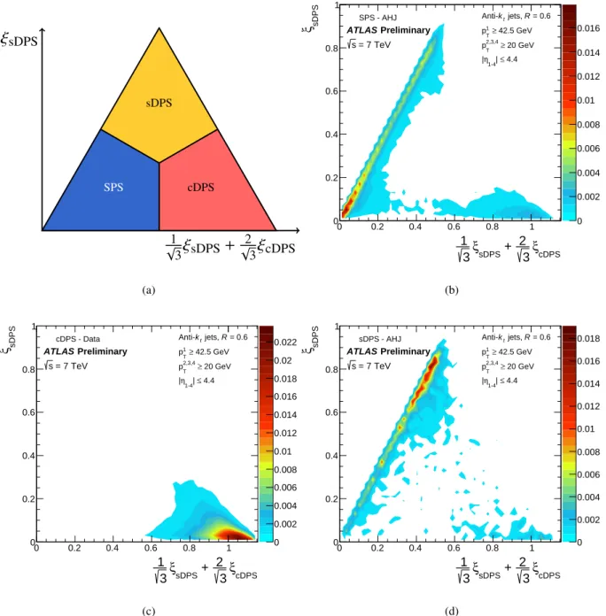
The NN used is a feed-forward multilayer perceptron with two hidden layers, implemented in the Root analysis framework [64]. The input layer has 21 neurons, corresponding to the variables defined in Eq. (15), and the first and second hidden layers have 30 and nine neurons, respectively. The output layer of the NN consists of three outputs, corresponding to three probabilities for the event to be SPS ( ξ

), cDPS ( ξ

) or sDPS ( ξ

). For each event, the three outputs are plotted as a single point inside an equilateral triangle (Dalitz plot) using the constraint ξ

+ ξ

+ ξ

= 1. A point in the triangle expresses the three probabilities as three distances from each of the sides of the triangle. The vertices would therefore be populated according to the probability to belong to one of the samples. Figure 3(a) shows an illustration of the Dalitz plot, where the horizontal axis corresponds to

3

ξ

+

3

ξ

and the vertical axis to the value of ξ

. The colored areas illustrate where each of the three classes of events is expected to populate the Dalitz plot.

The separation power of the NN is presented in the distributions of the three samples in the Dalitz plot, as shown in Figs. 3(c), (b) and (d). Events in the SPS sample are mostly classified as expected, with a sharp peak visible in the bottom left corner in Fig. 3(b). However, a contribution from SPS events in the bottom right corner is also visible. A ridge of SPS events extending towards the sDPS corner is observed as well. The clearest peak is seen for events from the cDPS sample in the bottom right corner in Fig. 3(c).

A visible cluster of sDPS events is seen in Fig. 3(d), concentrated around ξ

∼ 0 . 8 and there is a tail of events along the side connecting the SPS and sDPS corners.

Based on these observations, it is clear that event classification on an event-by-event basis is indeed impossible. However, the peak structure suggests that an estimation of the different contributions can be performed. To estimate the cDPS and sDPS fractions in four-jet events, the two-dimensional Dalitz distribution in data ( D ) is fitted to a weighted sum of the two-dimensional Dalitz distributions in the SPS ( M

), cDPS ( M

) and sDPS ( M

) samples, each normalized to the measured four-jet cross- section in data, with the fractions as free parameters. The optimal fractions are obtained using a fit of the form,

D = ( 1 − f

− f

) · M

+ f

· M

+ f

· M

, (17) where a χ

minimization is performed, as implemented in the Minuit package in Root [64], taking into account statistical uncertainties of all the samples in each bin.

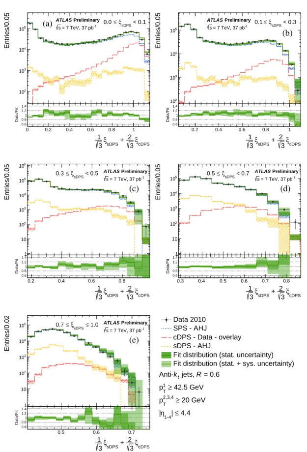
In order to visualize the results of the fit, the triangle is divided into five slices, 1. 0 . 0 ≤ ξ

< 0 . 1,

2. 0 . 1 ≤ ξ

< 0 . 3, 3. 0 . 3 ≤ ξ

< 0 . 5, 4. 0 . 5 ≤ ξ

< 0 . 7, 5. 0 . 7 ≤ ξ

≤ 1 . 0.

The fit is performed in two dimensions, but the fit results and NN output distributions are shown in the

one-dimensional slices. The results of the fit are shown in Fig. 5 in Section 7.

√1

3

ξ

+

3

ξ

ξ

SPS cDPS

sDPS

(a)

ξcDPS

3 + 2 ξsDPS

3 1

0 0.2 0.4 0.6 0.8 1

sDPSξ

0 0.2 0.4 0.6 0.8 1

0 0.002 0.004 0.006 0.008 0.01 0.012 0.014 0.016 Preliminary

ATLAS = 7 TeV s

SPS - AHJ Anti-k_t jets, R = 0.6 42.5 GeV

≥ 1 pT

20 GeV

≥ 2,3,4 pT

≤ 4.4 1-4| η

|

(b)

ξcDPS

3 + 2 ξsDPS

3 1

0 0.2 0.4 0.6 0.8 1

sDPSξ

0 0.2 0.4 0.6 0.8 1

0 0.002 0.004 0.006 0.008 0.01 0.012 0.014 0.016 0.018 0.02 0.022 Preliminary

ATLAS = 7 TeV s

cDPS - Data Anti-k_t jets, R = 0.6 42.5 GeV

≥ 1 pT

20 GeV

≥ 2,3,4 pT

≤ 4.4 1-4| η

|

(c)

ξcDPS

3 + 2 ξsDPS

3 1

0 0.2 0.4 0.6 0.8 1

sDPSξ

0 0.2 0.4 0.6 0.8 1

0 0.002 0.004 0.006 0.008 0.01 0.012 0.014 0.016 0.018 Preliminary

ATLAS = 7 TeV s

sDPS - AHJ Anti-k_t jets, R = 0.6 42.5 GeV

≥ 1 pT

20 GeV

≥ 2,3,4 pT

≤ 4.4 1-4| η

|

(d)

Figure 3: (a)Illustration of the Dalitz plot constructed from three NN outputs,ξ_SPS,ξ_cDPS, andξ_sDPS, with the constraint,ξ_SPS+ξ_cDPS+ξ_sDPS=1. The vertical and horizontal axes are defined in the figure. The colored areas illustrate the zones closest to the corresponding vertex.(b)-(d)Normalized distributions of the NN outputs, mapped to a two-dimensional Dalitz plot as described in the text, in the(b)SPS,(c)cDPS and(d)sDPS test samples selected in the phase-space defined in the legend.

5.4 Methodology validation

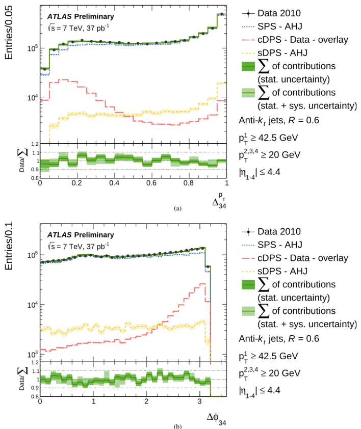
A sizable discrepancy was found in the ∆

34

and ∆ φ

distributions between the data and AHJ (see Fig. 8 in the Appendix), suggesting that there are more sub-leading jets (jets 3 and 4) which are back-to-back in AHJ than in the data. In order to test that the discrepancies are not from mis-modelling of SPS in AHJ, the ∆

34

and ∆φ

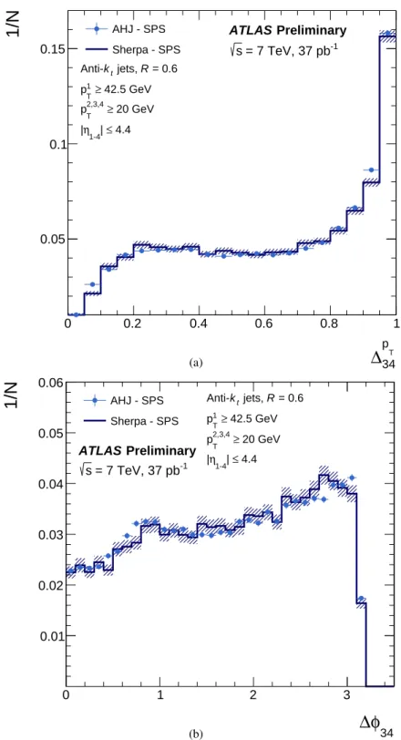
distributions in the SPS sample extracted from AHJ were compared to the distributions in the SPS sample generated in Sherpa (see Fig. 9 in the Appendix). A good agreement in the shapes of the distributions was observed for both variables. This and further studies performed indicate that the excess of events with jets 3 and 4 in the back-to-back topology is due to an excess of DPS events in the AHJ sample compared to the data.

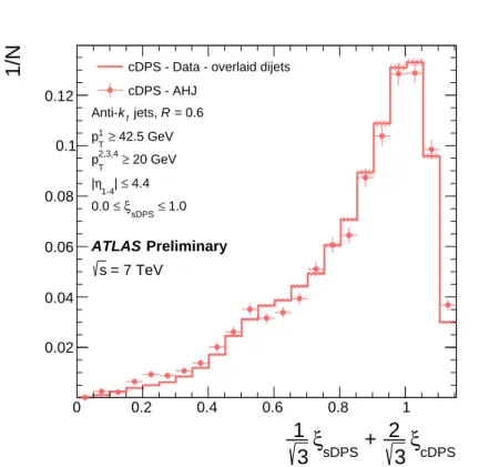
In order to verify that the topology of cDPS events is reproducible by overlaying two dijet events, the dijet overlay sample is compared to the cDPS sample extracted from AHJ. An extensive comparison between all the data and AHJ distributions used as inputs to the NN was performed and good agreement was observed. This can be summarised by comparing the NN output distributions. The NN is applied to the cDPS sample extracted from AHJ and the output distribution is compared to the output distribution of the cDPS sample constructed from dijets in data. Normalized distributions of the projection of the full Dalitz plot on the horizontal axis are shown in Fig. 4, where a good agreement is observed between the two distributions. Based on these results, it is concluded that the topology of the four jets in the overlaid dijet events is comparable to that of the four leading jets in cDPS events extracted from AHJ. An additional advantage of using overlaid dijets from data to construct the cDPS sample is that the jets are at the same JES as the jets in four-jet events in data. This leads to a smaller systematic uncertainty in the final result.

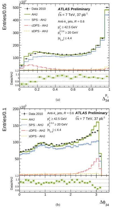
As an additional validation step, the NN is applied to the inclusive AHJ sample and the resulting distribution is fitted with the NN output distributions of the SPS, cDPS and sDPS samples (see Fig. 10 in the Appendix).

The fractions obtained from the fit, f

cDPS

and f

sDPS

, are compared to the fractions at parton-level, f

cDPS

and f

sDPS

, extracted from the event record, f

cDPS

= 0 . 094 ± 0 . 001 (stat.) , f

cDPS

= 0 . 094 ± 0 . 003 (stat.) , f

sDPS

= 0 . 048 ± 0 . 001 (stat.) , f

sDPS

= 0 . 041 ± 0 . 008 (stat.) .

(18)

The values obtained from the fit agree within their statistical uncertainties with those at parton-level. The larger statistical uncertainties on f

cDPS

and f

sDPS

obtained by the fit reflect the loss of statistical power due to the use of a template fit to estimate the fractions and the fact that their uncertainties are fully correlated.

6 Uncertainties

The combined statistical uncertainty on σ

is determined by performing many pseudo-experiments,

∆σ

=

%. The statistical uncertainty on α

2j

(of ∼ 1%) is propagated as a systematic uncertainty on

σ

. The systematic uncertainties associated with the integrated luminosity measurement ( ± 3 . 5%), the

re-weighting of AHJ ( ± 6%), the jet reconstruction efficiency ( ± 0 . 1%) and the selection of single-vertex

events ( ± 0 . 1%) are added in quadrature to the uncertainty on σ

. The combined uncertainty on σ

due to the jet energy resolution uncertainty and the jet angular resolution uncertainties is ± 12%. Various

sources of uncertainty on the JES are considered [57] and their combined contribution amounts to

%.

ξ

3 + 2 ξ

3 1

0 0.2 0.4 0.6 0.8 1

1/N

0.02 0.04 0.06 0.08 0.1 0.12

Preliminary ATLAS

= 7 TeV s

cDPS - Data - overlaid dijets cDPS - AHJ

= 0.6 R jets, kt

Anti-

42.5 GeV

≥

1

pT

20 GeV

≥

2,3,4

pT

≤ 4.4

1-4| η

|

≤ 1.0 ξsDPS

≤ 0.0

Figure 4: Normalized distributions of the NN outputs,^√1

3ξ_sDPS+^√2

3ξ_cDPS, in the range 0.0≤ξ_sDPS≤1.0 in cDPS events extracted from AHJ (red dots), selected in the phase space defined in the figure, and in the cDPS sample constructed from dijet events in data (red histogram).

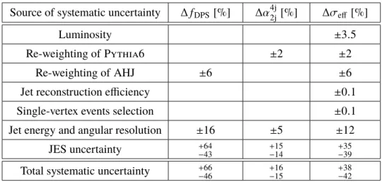
The relative systematic uncertainties on f

, α

2j

and σ

are summarized in Table 1. The dominant systematic uncertainty on f

originates from the JES variation, mainly through large variations of f

. A variation in the JES results in modified NN output distributions in the sDPS and SPS templates used in the fit to extract f

and f

. Due to the difficulty in differentiating between the sDPS and SPS topologies, and in particular the dependence on the transverse momentum of the fourth jet, the f

value changes substantially when using distributions that are modified by the JES variation.

The stability of the measured value of σ

with respect to the various parameter values used in the measurement was studied. Parameters such as p

T

and ∆R

were varied and the requirement

∆R

≤ 0 . 6 was applied, leading to a relative change in σ

of the order of a few percent. A

full study of the effects of these parameter values is not possible, as it would require repeating the

measurement using a different set of observables, e.g., anti- k

jets with a distance parameter of 0.4 or

generating a new AHJ sample with a different matching scale. However, since the observed relative

changes are small compared to the statistical uncertainty on σ

, no systematic uncertainty is assigned

due to these parameters.

Source of systematic uncertainty ∆ f

[%] ∆ α

2j

[%] ∆ σ

[%]

Luminosity ± 3 . 5

Re-weighting of Pythia6 ± 2 ± 2

Re-weighting of AHJ ± 6 ± 6

Jet reconstruction efficiency ± 0 . 1

Single-vertex events selection ± 0 . 1

Jet energy and angular resolution ± 16 ± 5 ± 12

JES uncertainty

Total systematic uncertainty

Table 1: Summary of the relative systematic uncertainties on f_DPS,α^4j

2jandσ_eff.

7 Determination of σ

To determine f

and σ

and their statistical uncertainties taking into account all of the correlations, many pseudo-experiments (fits) are performed. The systematic uncertainties are obtained by propagating the expected variations into the analysis and the resulting shifts are added in quadrature. The result for

f

is

f

= 0 . 084

(stat.)

(syst.) , (19) where the systematic uncertainties on f

are detailed in Table 1. The intermediate results for f

and

f

can be quantified as

f

= 0 . 052

(stat.) ± 0 . 008 (syst.) , f

= 0 . 032

(stat.)

(syst.) , (20) where the quoted systematic uncertainties do not include any positivity constraint on the fractions. When taking into account the systematic uncertainties of the templates in the calculation of the goodness-of-fit χ

(without re-doing the fit), a value for χ

/ NDF of 0.7 is obtained, where NDF is the number of degrees of freedom of the fit. This indicates that the sum of the SPS, cDPS and sDPS contributions after the fit has been performed provides a good description of the data.

A comparison of the fit distributions with the distributions in data in five one-dimensional slices of the Dalitz plot is shown in Fig. 5. The statistical uncertainty in each bin in the fit distribution is shown as the dark shaded area while the light shaded area represents their sum in quadrature with the systematic uncertainties. The distributions of the SPS, cDPS and sDPS contributions are also shown, normalized to their respective fraction in the data as obtained by the fit. Considering the systematic uncertainties, the most significant disagreement with the data is seen for the left-most bin in the range 0 . 0 ≤ ξ

< 0 . 1 (Fig. 5(a)) of the Dalitz plot. This bin is dominated by the SPS contribution. Thus, a discrepancy between the data and the fit result in this bin is expected to have a negligible effect on the measurement of the double parton scattering rate.

The distributions of the ∆

34

and ∆φ

variables in data are compared to a combination of the distributions

in the three samples, SPS, cDPS and sDPS in Fig. 6. The latter three distributions are normalized to their

respective fraction in the data as obtained by the fit. A good description of the data is achieved.