ATLAS NOTE ATLAS-CONF-2016-042

A TLAS-CONF-2016-042 08 August 2016

ATLAS NOTE

ATLAS-CONF-2016-042

2nd August 2016

Search for long-lived neutral particles decaying into displaced lepton-jets in proton–proton collisions at √

s = 13 TeV with the ATLAS detector

The ATLAS Collaboration

Abstract

This note presents the results of a search for long-lived neutral particles decaying into collimated jets of light leptons and mesons, so-called “lepton-jets”, using a sample of 3.4 fb

of proton-proton collisions data at a centre-of-mass energy of

√ s =13 TeV collected during 2015 with the ATLAS detector at the LHC. No deviations from Standard Model expectations are observed. Limits on models predicting Higgs boson decays to neutral long-lived particles (dark photons γ

), which in turn produce lepton-jets, are derived as a function of the particle proper decay length, c τ . Assuming the Standard Model gluon-fusion production cross section for a 125 GeV Higgs boson, its branching ratio to dark photons is found to be below 10%, at 95% CL, for dark-photon lifetimes in the range 2.2 ≤ c τ ≤ 111.3 mm in a Higgs → 2 γ

+ X benchmark model and in the range 3.8 ≤ c τ ≤ 163 mm in a Higgs → 4 γ

+ X model. These limits improve upon the results of a similar search previously performed during Run 1 of the LHC, due to enhancements in the trigger and reconstruction of highly-collimated muons.

© 2016 CERN for the benefit of the ATLAS Collaboration.

Reproduction of this article or parts of it is allowed as specified in the CC-BY-4.0 license.

1 Introduction

Several possible extensions of the Standard Model (SM) predict the existence of a dark sector that is weakly coupled to the visible one [1–6]. Depending on the structure of the dark sector and its coupling to the SM, some unstable dark states may be produced at colliders and decay back to SM particles with sizeable branching fractions.

An extensively studied case is one in which the two sectors couple via the vector portal, where a dark photon ( γ

) with mass in the MeV to GeV range mixes kinetically with the SM photon [7–9]. If the dark photon is the lightest state in the dark sector, it will decay to SM particles, mainly to leptons and possibly light mesons. Due to its weak interactions with the SM, it can have a non-negligible lifetime.

At the LHC, these dark photons would typically be produced with large boost, due to their small mass, resulting in collimated jet-like structures containing pairs of leptons and/or light hadrons (lepton-jets, LJs). If produced away from the interaction point (IP), they are referred to as “displaced LJs”. In this note, the search is limited to displaced LJs, and the LJ constituents are limited to electrons, muons, and pions.

Electrically neutral particles which decay far from the IP into collimated final states represent a challenge both for the trigger and for the reconstruction capabilities of the ATLAS detector. Collimated charged particles in the final state can be difficult to reconstruct, due to the limited granularity of the detector. For decays displaced far enough from the IP to occur past the inner tracking system, only information from the calorimeters – and in the case of final-state muons, the Muon Spectrometer (MS) – is available for the reconstruction of the decay products.

The high-resolution, high-granularity measurement capability of the ATLAS “air-core” MS is ideal for this type of search. In addition, the ATLAS inner tracking system, despite not being used for the physics object definition, can be used to define track isolation criteria useful to significantly reduce the otherwise overwhelming SM background.

The search for displaced LJs presented in this note employs the full dataset collected by ATLAS during 2015 at

√ s = 13 TeV, corresponding to an integrated luminosity of 3.4 fb

. Similar searches were performed using the data collected by ATLAS in 2011 and 2012 at 7 and 8 TeV respectively [10, 11].

Related searches for prompt LJs have been performed both at the Tevatron [12, 13] and at the LHC [14–16].

Additional constraints on scenarios with dark photons are extracted from, e.g., beam-dump and fixed- target experiments [17–26], e

e

colliders [27–29], B-factories [30, 31], electron and muon anomalous magnetic moment measurements [32–34] and astrophysical observations [35, 36].

The properties of the LJ, such as its shape and particle multiplicity, strongly depend on the unknown structure of the dark sector and its couplings to the visible sector. Therefore the search criteria are designed to be as model-independent as possible, targeting the basic experimental signatures that correspond to these objects. A mapping of the results of this search onto a specific model can then follow.

The analysis strategy divides the various LJs into categories based on the species of the constituent particles. For each category, LJs are defined using a basic clustering algorithm with a cone of a fixed angular size. Dedicated triggers that are not linked to the interaction point position are employed to target the displaced decays. The main backgrounds to the analysis are multijet production, cosmic-ray muons, and beam halo. A strict set of selection requirements is chosen to optimise the signal significance. A combination of Monte Carlo (MC) and data-driven techniques is used to evaluate the residual backgrounds.

Despite the lower integrated luminosity of the 2015 dataset at

√ s = 13 TeV compared to the 2012 dataset

at 8 TeV, the sensitivity to displaced LJ signatures is comparable. This is due to the improvements in the

trigger and reconstruction efficiencies for collimated muons. In addition, larger production cross-sections

are expected at 13 TeV than at 8 TeV for a wide variety of physics models with LJ signatures. For example,

the gluon–gluon fusion Higgs production cross section is higher by a factor of approximately 2.3 [37], leading to increased expected production of LJs in models where dark photons appear in decay chains starting from a Higgs.

The LJ definition and two simplified benchmark models for LJ production are presented in Section 2. A brief description of the ATLAS detector follows in Section 3. The signature and the search criteria used to select LJs are discussed in Section 4 and Section 5. Section 6 describes two additional cuts imposed at event level to improve the selection of LJs. In the Section 7 the acceptance time reconstruction efficiency for the signal models is reported. The final results, the residual background evaluated using a data-driven method and the systematic uncertainties on the search, are presented in Section 8. The results of the search are also used to set upper limits on the product of cross section and Higgs decay branching fraction to LJs, as a function of the dark photon ( γ

) mean lifetime. Section 9 summarizes the results of this search.

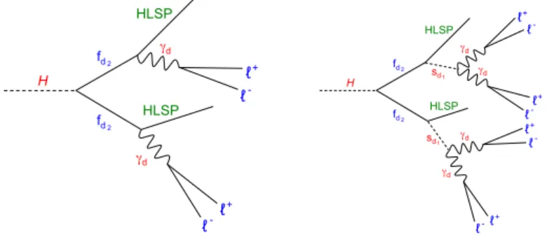
2 Signal benchmark models

Amongst the numerous models predicting γ

, one class particularly interesting for the LHC features the hidden sector communicating with the SM through the Higgs portal. The two benchmark models used in this analysis are the Falkowsky-Ruderman-Volansky-Zupan (FRVZ) models [8, 9] where the Higgs boson decays to a pair of hidden fermions f

. As shown in Figure 1, the first benchmark model produces two γ

while the second produces four γ

. In the first benchmark model (left), the dark fermion decays to a γ

and a lighter dark fermion f

, assumed to be the HLSP (Hidden Lightest Stable Particle). In the second model (right), the dark fermion f

decays to an HLSP and a dark scalar s

that in turn decays to pairs of dark photons. In general, dark sector radiation can produce extra dark photons, but the number

γd

H f_d2

fd₂

γd

HLSP

HLSP

ℓ ⁺ ℓ ^-

ℓ ⁺ ℓ ^-

γd H

fd2

f_d2 γd HLSP

HLSP

γd γd sd1

s_d1

ℓ ⁺ ℓ ^-

ℓ ⁺ ℓ ^-

ℓ ⁺ ℓ ^-

ℓ ⁺ ℓ ^-

Figure 1: The two FRVZ models used as benchmarks in the analysis. In the first model (left), the dark fermion decays to a γ

and a HLSP. In the second model (right), the dark fermion f

decays to an HLSP and a dark scalar s

that in turn decays to pairs of dark photons.

produced is model-dependent because the number of radiated dark photons is proportional to the size of the dark gauge coupling α

(see, for example, equation 3.1 in [7].) The dark radiation is not included in the signal MC, which corresponds to assuming weak dark coupling, α

. 0 . 01.

A low-mass dark photon mixing kinetically with the SM photon will decay mainly to leptons and possibly light mesons, with branching fractions that depend on its mass [8, 38, 39]. In the models considered, the decays to tau-leptons are not included. The γ

decay lifetime, τ (expressed throughout this note as τ times the speed of light c ), is controlled by the kinetic mixing parameter, [39] and is a free parameter of the model. The set of parameters used to generate the signal MC is listed in Table 1. The Higgs boson is generated through the gluon–gluon fusion production mechanism, the dominant process for a low-mass Higgs. The gluon–gluon fusion Higgs boson production cross section in pp collisions at

√ s = 13 TeV,

estimated at the next-to-next-to-leading order (NNLO) [40], is σ

= 43.87 pb for m

= 125.09 GeV. The masses of f

and f

are chosen to be light relative to the Higgs boson mass, and far from the kinematic threshold at m

d1/LSP

+ m

d

= m

d2

. For the chosen dark-photon mass (0.4 GeV), the γ

decay branching ratios ( BR ) are expected to be 45% e

e

, 45% µ

µ

, 10% π

π

[8]. The mean lifetime τ of the γ

is a free parameter of the model. In the generated samples c τ is chosen such that, accounting for the boost of the γ

, a large fraction of the decays occurs inside the sensitive ATLAS detector volume (i.e. up to 7 m in radius and 13 m along the z -axis, where the muon trigger chambers are located.) The detection efficiency can then be estimated for a range of γ

mean lifetimes through reweighting of the decay position in the generated samples. A second set of MC events with a Higgs-like scalar at high mass (800 GeV), and the same decay chain, has also been simulated.

The MG5_aMC@NLO v2.2.3 generator [41], linked together with the PYTHIA8 generator [42] v8.186, is used for gluon–gluon fusion production of the Higgs boson and the subsequent decay to dark-sector particles.

The generated Monte Carlo events are processed through the full ATLAS simulation chain based on GEANT4 [43, 44] and then reconstructed and processed in the same manner as the data.

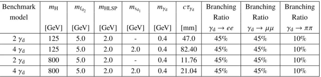
Benchmark m

m

d2

m

m

d1

m

d

cτ

d

Branching Branching Branching

model Ratio Ratio Ratio

[GeV] [GeV] [GeV] [GeV] [GeV] [mm] γ

→ ee γ

→ µµ γ

→ ππ

2 γ

125 5.0 2.0 - 0.4 47.0 45% 45% 10%

4 γ

125 5.0 2.0 2.0 0.4 82.40 45% 45% 10%

2 γ

800 5.0 2.0 - 0.4 11.76 45% 45% 10%

4 γ

800 5.0 2.0 2.0 0.4 21.04 45% 45% 10%

Table 1: Parameters used for the Monte Carlo simulation, for m

= 125 and m

= 800 GeV. The first and the third rows are for the 2 γ

final state (first benchmark model). The second and fourth rows are for the 4 γ

final state (second benchmark model). Each dataset consists of approximately 300000 events.

3 ATLAS detector

ATLAS is a multi-purpose detector [45] at the LHC, consisting of an inner tracking system (ID) contained in a superconducting solenoid, which provides a 2 T magnetic field parallel to the beam direction, electromagnetic and hadronic calorimeters (EMCAL and HCAL) and a muon spectrometer (MS) that has a system of three large air-core toroid magnets.

The ID combines high-resolution detectors at the inner radii with continuous tracking elements at the outer radii. It provides measurements of charged-particle momenta in the region of pseudorapidity1

|η | ≤ 2.5. The highest granularity is obtained around the interaction point using semiconductor pixel detectors arranged in four barrel layers and three disks on each side2, followed by four layers of silicon microstrip detectors and a transition radiation tracker.

1

ATLAS uses a right-handed coordinate system with its origin at the nominal interaction point in the centre of the detector and the

-axis coinciding with the beam pipe axis. The

-axis points from the interaction point to the centre of the LHC ring, and the

-axis points upward. Cylindrical coordinates (

,φ) are used in the transverse plane,

being the azimuthal angle around the beam pipe. The pseudorapidity is defined in terms of the polar angle

as

=

ln tan(

/2).

2

The outermost barrel layer has an average radius 12.25 cm, and the outermost endcap layer at

65 cm. The innermost

barrel layer, composed by planar and 3D pixel sensors, is the Insertable B-layer (IBL).

The EMCAL and HCAL calorimeters cover |η | ≤ 4.9, and have a total depth of 22 radiation lengths and 9.7 interaction lengths, respectively, at η = 0. The barrel EMCAL starts at a radial distance of 1.44 m and ends at 1.90 m with a z extension of ± 3.21 m, covering the |η | ≤ 1 . 5 interval. The barrel HCAL starts at a radial distance of 2.20 m and ends at 3.72 m with a z extension of ± 4.10 m, with the same η -coverage of the EMCAL. The EM endcap part starts at z ± 3.70 m and ends at ± 4.25 m and the HCAL part starts immediately after the EM part and ends at ± 5.98 m with an |η | coverage up to 4.8.

The muon spectrometer (MS) provides trigger information ( |η | ≤ 2.4) and momentum measurements ( |η | ≤ 2.7) for charged particles. It consists of one barrel ( |η| ≤ 1.05) and two endcaps (1 . 05 ≤ |η | ≤ 2 . 7), each with 16 sectors in φ , equipped with fast detectors for triggering and with chambers measuring the tracks of the outgoing muons with high spatial precision. The MS detectors are arranged in three stations at increasing distance from the IP: inner, middle and outer. Monitored drift tubes are used for tracking in the region |η | ≤ 2.7, except for the innermost layer of endcaps which uses cathode strip chambers in the interval 2.0 ≤ |η | ≤ 2.7. The toroidal magnetic field allows for precise reconstruction of charged-particle tracks independent of the ID information. The three planes of MS trigger chambers (resistive plate chambers in the barrel and thin gap chambers in the endcaps) are located in the middle and outer (only in the barrel) stations.

The trigger system has two levels [46] called Level-1 (L1) and High-Level Trigger (HLT). The L1 is a hardware-based system using information from the calorimeters and MS. It defines one or more region-of- interest (RoIs), geometrical regions of the detector, identified by ( η , φ ) coordinates, containing interesting physics objects. The HLT is a software-based system and can access information from all sub-detectors.

The L1 muon trigger requires hits in the middle stations to create a low transverse momentum ( p

) muon RoI or hits in both the middle and outer stations for a high- p

muon RoI. The muon RoIs have a spatial extent of 0.2 × 0.2 ( ∆η × ∆φ ) in the barrel and of 0.1 × 0.1 ( ∆η × ∆φ ) in the endcaps. L1 RoI information seeds the reconstruction of muon momenta by the HLT, which uses precision chamber information.

4 Lepton-jet object definition

In the benchmark models considered for this study, the dark photons are produced from the decays of heavy particles and two LJs are expected to be produced back-to-back in the azimuthal plane. In this Section the single LJ definition and reconstruction is described.

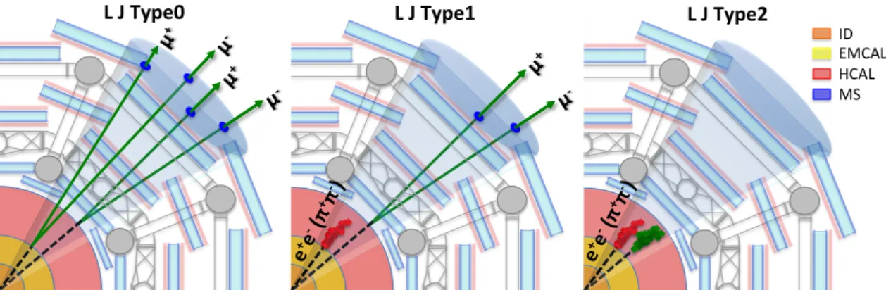
LJs are defined and classified according to the muon and/or jet content found within a cone of opening

∆R = p

(∆η)

+ (∆φ)

and satisfying dedicated selection criteria. If at least two muons and no jets are found in the cone, the LJ is classified as Type0. Otherwise, if there are at least two muons and only one jet in the cone, the LJ is of Type1. The remaining jets satisfying the selection criteria, and with no muons in their cones, are defined as Type2 LJs. The LJ four-momentum is obtained from the vector sum over all momenta of constituents of the LJ. Figure 2 schematically shows the LJ classification. Limiting the search to γ

displaced decays greatly reduces the SM background. Muonic LJs decays are defined as “displaced”

if the decay happens beyond the last pixel detector layer and uses muons reconstructed using only MS information. The ATLAS standard muon reconstruction [47] matches the muon tracks in the MS to ID tracks to form combined muons. Since the ID track reconstruction in ATLAS requires at least one hit in the ID pixel layers, the use of non-combined muons rejects muons coming from the main proton-proton interaction point. The search is limited to the pseudorapidity interval |η| < 2 . 4 corresponding to the ID and muon trigger coverage. Tracks in the |η | interval 1.0 to 1.1 are rejected, avoiding the magnetic field transition region in the MS between barrel and endcap.

Muonic LJs are reconstructed using a simple clustering algorithm that combines all the muons lying within

Cone%of%opening%angle%ΔR%

J%%TYPE0%

L% L J Type0

Cone%of%opening%angle%ΔR%

J%%TYPE1%

L% L J Type1

Cone%of%opening%angle%ΔR%

ID#EMCAL#

HCAL#

MS#

J%%TYPE2%

L% L J Type2

Figure 2: Schematic picture of the LJ classification according to the γ

decay final states. Electrons and pions originating from γ

decay appear as jets. Type0 LJ is composed of only muons (left). Type1 LJ is composed of muons and a jet (centre). Type2 LJ is composed of only jets (right).

a cone of a fixed ∆R . The algorithm is seeded by the highest- p

muon. If at least two muons are found in the cone, the LJ is accepted. The search is then repeated with any unassociated muon until no muon seed is left. For Type0 LJs, the size of the search cone is optimised using the distribution of the maximum opening angle between the muons or between muons and jets in the benchmark model MC. It is found that for the benchmark models considered in this analysis, a cone size of ∆R = 0.5 contains all the dark photons decay products.

For the Type2 LJs an anti- k

calorimetric jet search algorithm [48], with the radius parameter R = 0.4, is used to select γ

decaying into an electron or pion pair. Jets must satisfy the standard ATLAS quality selection criteria [49] with the requirement p

≥ 20 GeV. The otherwise standard requirement on the electromagnetic (EM) fraction, defined as the ratio of the energy deposited in the EM calorimeter to the total jet energy, is removed to accommodate decays in the HCAL. The jet energy scale correction as defined in [50] is applied. LJs produced by a single dark photon decaying into an electron/pion pair and LJs containing two dark photons, each decaying to an electron/pion pair, are always expected to be reconstructed as a single jet due to their large boost.

5 Event preselection and background rejection

Data used for this analysis were collected during the entire 2015 data taking period, where only runs in which all the ATLAS subdetectors were running at nominal conditions are selected.

5.1 Triggers

A large fraction of the standard ATLAS triggers [46] are designed assuming prompt production and therefore are very inefficient in selecting the products of displaced decays. The logical OR of the following dedicated triggers is used:

• Narrow-Scan: The Narrow-Scan trigger was introduced for the 2015 data-taking, and adopts a

specialised and novel approach for a wide range of signal models featuring highly collimated muons

such as in the LJ case. The Narrow-Scan algorithm begins with requiring at least one L1 trigger

muon object. Other multi-muon triggers, which usually require more L1 trigger muon objects, have

large associated signal efficiency losses in the case where the muons are produced close together.

These losses are mainly due to the limited granularity at L1, resulting in fewer reconstructed L1 muon objects than “real” muons, and due to the inevitable matching ambiguity between the L1 and the HLT muon objects. To compensate for the high rate from only one L1 muon object (which is fully matched at HLT), a “scan” is performed for another muon at HLT without requiring it to match a L1 muon object. To limit the online resources consumption, the scan is limited to a narrow cone around the previously fully matched muon, where e.g. other constituents of the lepton-jet are expected to be found. In the trigger used in this analysis, neither of the fully matched HLT muons is required explicitly to have a matching ID track, while the “scanned” muon is explicitly required to be unmatched to an ID track. In this analysis the trigger is implemented such that the fully matched muon must have p

≥ 20 GeV, while the “scanned” muon must lie in the a cone of ∆R = 0 . 5 around the leading muon and have p

≥ 6 GeV.

• Tri-muon MS-only [51]: selects events with at least three MS-only muons with p

≥ 6 GeV. It is seeded at L1 by a cluster of three muon ROIs in a ∆R = 0.4 cone, and is required to have no reconstructed jets within a cone of ∆R = 0.5.

• CalRatio [51]: selects events with an isolated jet of low EM fraction. The CalRatio trigger is seeded by a L1 tau-lepton trigger with p

≥ 60 GeV. A L1 tau-lepton seed was chosen over a jet seed because the L1 τ seed uses a narrower calorimeter region than the L1 jet seed. Decays of γ

in the HCAL tend to produce narrow jets. The trigger requires the jet to have |η| ≤ 2 . 4 (to ensure that ID tracks can be matched to it) and E

≥ 30 GeV. A selection requirement on the calorimeter energy ratio is then imposed, requiring log (E

/E

) ≥ 1 . 2. Finally, ID track isolation selection around the jet axis (no track with p

≥ 2 GeV within ∆R ≤ 0 . 2 from the jet axis) and BIB tagging are performed to reject fake jets from beam-halo muons.

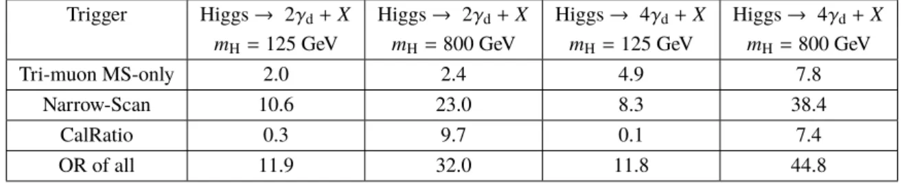
The resulting trigger acceptance times efficiencies on the benchmark models, defined as the ratio between the number of triggered events and the total number of MC generated ones, are shown in Table 2. The Narrow-Scan trigger, which was not available in Run 1, provides a large increase in trigger efficiency. The CalRatio trigger has lower efficiency for this analysis in Run 2, due to the increased minimum tau-lepton p

threshold at L1.

Trigger Higgs → 2 γ

+ X Higgs → 2 γ

+ X Higgs → 4 γ

+ X Higgs → 4 γ

+ X m

= 125 GeV m

= 800 GeV m

= 125 GeV m

= 800 GeV

Tri-muon MS-only 2.0 2.4 4.9 7.8

Narrow-Scan 10.6 23.0 8.3 38.4

CalRatio 0.3 9.7 0.1 7.4

OR of all 11.9 32.0 11.8 44.8

Table 2: The acceptance times efficiency (in %) of the triggers for MC of the benchmark processes.

5.2 Rejection of cosmic-ray muons background

Cosmic-ray muons that cross the detector in time coincidence with a pp interaction constitute the main source of background to the Type0 signal, and a sub-dominant background to the Type1 and Type2 signals.

A sample of events collected in the empty bunch-crossings (bunches not filled with protons) with the same

triggers as in the 2015 collision data is used to study this background.

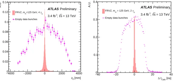
To reduce contamination of LJ Type0 and Type1 by cosmic-ray muons, a selection requirement on the longitudinal muon track impact parameter | z

| is used, where | z

| is defined as the minimum distance in the z -coordinate of the non-combined muon track to the primary interaction vertex. The primary interaction vertex is defined to be the vertex whose constituent tracks have the largest Σp

T

. Figure 3 (left) shows the | z

| distributions for muonic LJ constituents in empty bunch-crossings (cosmic-ray muons) of the 2015 data taking, and in the m

= 125 GeV FRVZ Higgs → 4 γ

+ X sample. (Amongst the FRVZ samples, the Higgs → 4 γ

+ X exhibits the widest |z

| distribution, due to the lower LJ boost.) A selection requirement | z

| ≤ 280 mm is used; in this way only 5% of the signal in the Higgs → 4 γ

+ X sample is lost while eliminating 96% of the cosmic-ray background. Energy deposits from hard bremsstrahlung of

[mm]

z0

−4000 −2000 0 2000 4000

A.U.

0 0.02 0.04 0.06 0.08 0.1 0.12 0.14

γd

=125 GeV, 4 FRVZ, mH

Empty data bunches

Preliminary ATLAS

= 13 TeV s

-1, 3.4 fb

[ns]

tCalo

∆

−40 −20 0 20 40

A.U.

0 0.1 0.2 0.3 0.4

γd

= 125 GeV, 2 FRVZ, mH

Empty data bunches

Preliminary ATLAS

= 13 TeV s

-1, 3.4 fb

Figure 3: The muon impact parameter |z

| (left) for muonic LJ constituents in empty bunch-crossings (cosmic-ray muons) and for muonic LJ constituents in the m

= 125 GeV FRVZ Higgs → 4 γ

+ X case. The jet timing, ∆t

, (right) of Type2 LJs from signal MC and single jet triggered events in empty bunch-crossings. In both plots, data refers to the 2015 data taking.

cosmic-ray muons in the HCAL can be reconstructed as jets with low EM fraction, creating a background to the Type1 and Type2 LJ selections. The observable used to remove jets from cosmic-ray events is the jet timing ∆t

, defined as the energy-weighted mean time difference between the bunch-crossing time and the time of the energy deposition in the calorimeter cells. Figure 3 (right) shows that cosmic rays tend to have a wide ∆t

distribution, while the signal MC Type1 and Type2 jets have a narrow peak at the bunch-crossing time. Removing jets with ∆t

outside the interval between − 4 ns and +4 ns removes a large fraction of the cosmic-ray jets, with a loss of signal less than 5%.

5.3 Rejection of multijet production background

Multijet production constitutes the main background to the Type2 LJ signal. The search explicitly targets γ

decays in the HCAL, resulting in most of the energy deposition occurring in the HCAL rather than in the ECAL. Therefore, low EM fraction is an effective criterion to distinguish jets in Type1 and Type2 LJs from multijet background.

Another effective discriminating variable is the jet width W , defined as the average distance of a jet

constituent to the jet direction weighted with the energy of the constituent:

W = P

i

∆R

· p

T

P

i

p

T

, (1)

where ∆R

=

p ( ∆ φ

)

+ ( ∆ η

)

is the distance between the jet axis and the i

jet constituent and p

T

is the constituent p

with respect to the beam axis. The jet constituents are calorimeter clusters, as defined in [52].

In addition, a third discriminating variable is provided by the jet vertex tagger [53] (JVT), which exploits the sum of the p

of tracks associated with the jets from the primary interaction. The JVT selection requirement is designed to reject jets originating from pile-up, while retaining jets coming from the primary interaction; since Type2 LJs tend not to be associated with the primary interaction (due to their displacement), the JVT selection is used oppositely to its typical usage.

The selection requirements are optimised against the expected multijet background using a di-jet control sample from data. A tag-and-probe method is used with 1.0 fb

of the 2015 data. The leading jet in the event defines the “tag jet”, while the sub-leading is the “probe jet”. Only events that have both a tag and a probe jet with E

≥ 20 GeVand |η | ≤ 2.4 are considered. An additional requirement of ∆ φ ≥ 2 . 5 between the tag and the probe is imposed to select back-to-back topologies, which is expected in di-jet production.

The outcome of the optimization is:

• EM fraction < 0 . 1,

• W < 0 . 058,

• JVT < 0 . 56.

5.4 Rejection of background due to jets in HCAL transition region

A source of background jets with artificially low EM fraction consists of jets reconstructed in the crack region of the calorimeters, corresponding to the transition region between the barrel and end-cap cryostat.

These are removed by requiring the fraction of energy in the HCAL region between 1 . 0 < |η | < 1 . 6, where the HCAL consists of only scintillators (“tile-gap scintillators”), to be less than 0.1 of the total jet energy.

5.5 Rejection of beam-induced background

Beam-induced background (BIB), consisting of high energy beam-halo muons undergoing hard bremss-

trahlung in the calorimeters, is another sub-dominant source of background for Type2 LJs. The bremsstrah-

lung manifests itself as a calorimeter deposit that is reconstructed as a jet; if it occurs in the HCAL, the

fake jet is reconstructed with a very low EM fraction. BIB “tagging” searches for two track segments

parallel to the beam line in the forward MDT chambers, together with a low EM fraction HCAL jet, all

within 4 degrees in φ . Such an HCAL jet is tagged as BIB and removed from the data set.

5.6 Additional backgrounds

Apart from the backgrounds described in the previous sections, other potential backgrounds to our signal include all the processes which lead to real prompt muons and muons plus jets in the final state such as the SM processes W +jets, Z +jets, t t ¯ , single-top, WW , WZ, and ZZ . However, the main contribution to the background is expected from processes giving a high production rate of secondary muons which do not point to the primary vertex, such as decays in flight of K/π and heavy flavour decays in multijet processes, or muons due to cosmic-ray. ATLAS MC for these processes are used, and the generated MC events are processed through the full ATLAS simulation and reconstruction chain. The selection for LJ events is run on all the above MC, using a simulation of the same triggers used to collect data. After the previous described cuts, the events surviving are mainly Type1–Type1 and Type0–Type1, these events are fully removed by applying the additional cut on the muons of the LJ to be non-combined (“no-CB”).

5.7 Summary of preselection requirements

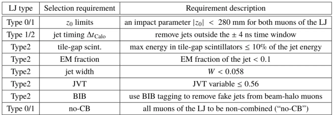
A summary of the LJ signal selection requirements is given in Table 3.

LJ type Selection requirement Requirement description

Type 0/1 z

limits an impact parameter |z

| < 280 mm for both muons of the LJ Type 1/2 jet timing ∆t

remove jets outside the ± 4 ns time window

Type2 tile-gap scint. max energy in tile-gap scintillators ≤ 10% of the jet energy Type2 EM fraction EM fraction of the jet < 0 . 1

Type2 jet width W < 0 . 058

Type2 JVT JVT variable ≤ 0.56

Type2 BIB use BIB tagging to remove fake jets from beam-halo muons Type 0/1 no-CB all muons of the LJ to be non-combined (“no-CB”)

Table 3: LJ signal selection requirements.

6 Completion of the event selection

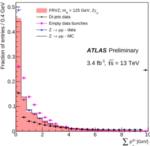
Two LJ objects passing the complete list of selection criteria in Table 3 are required in the event, and two additional requirements are then imposed at event level: ID track isolation, and ∆φ between the two LJs.

Displaced LJs are expected to be well isolated in the ID. Therefore the multijet background can be significantly reduced by requiring track isolation around the LJ direction in the ID. The track ID isolation Σp

T

is defined as the sum of the transverse momenta of the tracks with p

> 500 MeV, reconstructed in the ID and matched to the primary vertex of the event, inside a cone of size ∆R = 0.5 around the direction of the LJ. Matching to the primary vertex helps reduce the dependence of Σp

T

on the pile-up events.

The Σp

T

for the LJs from the benchmark models is very similar to that for muons from Z → µµ decays, and there is no significant difference in the behaviour of Σp

T

between the different LJ types; hence the behaviour of Σp

T

in Z → µµ is employed to study the behaviour of Σp

T

in the benchmark models. In order to verify that the Z → µµ MC models the Σp

T

accurately, the Σp

T

in this MC is compared to

that in 2015 data using muons from a selected sample of Z → µµ decays (Figure 4), removing the p

of the ID track matched to the muon. The level of disagreement between the Z → µµ data and MC, seen in the first bin of the histogram in Figure 4, is due to a possible mis-modelling of the underlying event and pileup and becomes negligible for Σp

T

>3 GeV. The Figure also shows the Σp

T

distribution for the LJs found in the di-jet control sample of 2015 data; the overflow events ( Σp

T

> 10 GeV) are filled in the last interval for illustration. Clearly Σp

T

is highly effective in distinguishing the LJ signal from the

[GeV]

ID T

∑

0 2 4 6 8 10

Fraction of entries / 0.4 GeV

0 0.1 0.2 0.3 0.4 0.5

γd

= 125 GeV, 2 FRVZ, mH

Di-jets data Empty data bunches

- data µ µ

→ Z

- MC µ µ

→ Z

Preliminary ATLAS

= 13 TeV s

-1, 3.4 fb

Figure 4: The distributions of Σp

T

for the 2015 data di-jet control sample (black circles), Z → µµ sample (blue triangles), and cosmic sample in empty bunch-crossings (violet squares). The similarity between Z → µµ distributions (in data and MC) and the signal distribution (solid red area) enables to use these distributions for validating the signal modelling in this variable. All distributions are normalized to unit area. The overflow events for the di-jet control sample ( Σp

T

> 10 GeV) are filled in the last interval.

multijet background. A selection is imposed on the maximum value of Σp

T

amongst all LJs in a given event; the criterion Max Σp

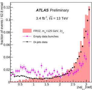
< 4.5 GeV greatly reduces the multijet background while maintaining a very high LJ signal selection efficiency. The two LJs in the FRVZ models are expected to be back-to-back in the transverse plane, as can be seen from the |∆φ| distribution between the two reconstructed LJs in the FRVZ 125 GeV Higgs → 2 γ

+ X MC (Figure 5). The multijet background remains flat at small angle.

Therefore, an additional selection requirement on the ∆φ between the two LJs in the azimuthal plane,

|∆φ|

> 0 . 63 rad, reduces the multijet background without significantly affecting the signal.

7 Lepton-jet signal selection efficiencies

In this section we address the efficiency for a γ

(or a collimated pair of dark photons from the decay of

a heavier dark sector particle, e.g. in the benchmark models described in Section 2) to be reconstructed

as one of the LJ types. For Type0 LJs, the γ

acceptance times reconstruction efficiency, defined as the

ratio between the number of γ

→ µµ reconstructed as LJs and the total number of γ

→ µµ in a given

interval of decay distance, is shown in Figure 6 as a function of the γ

transverse decay distance L

in the

barrel and of the longitudinal decay distance L

in the endcap, for the m

= 125 and 800 GeV samples.

[rad]

|LJ

φ

∆

0.5 1 1.5 2 2.5| 3

fraction of events / 62.8 mrad

0 0.02 0.04 0.06 0.08 0.1 0.12

γd

=125 GeV, 2 FRVZ, mH

Empty data bunches Di-jets data

Preliminary ATLAS

= 13 TeV s

-1, 3.4 fb

Figure 5: |∆φ| between the two reconstructed LJs from the FRVZ Higgs → 2 γ

+ X and Higgs → 4 γ

+ X benchmark MC. The mass of the Higgs boson is 125 GeV. For comparison the distribution of the cosmics sample from empty bunch-crossings data and that of di-jets from the control sample of 2015 data are superimposed. The uncertainties are statistical only.

The efficiency decreases with increasing distance from the interaction point, due to the decrease of the separation between the two muons in the innermost MDT stations. The increase in efficiency after the innermost chambers ( ∼ 4 . 5 m in the barrel, ∼ 7 . 5 m in the endcaps) is due to the separation of the two muons under the influence of the MS magnetic field.

The acceptance times efficiency for the m

= 800 GeV sample is systematically lower due to the higher boost of the γ

with the consequent decrease of the separation between the two tracks.

For Type2 LJs, the acceptance times reconstruction efficiency, defined as the ratio between the number of γ

→ ee ππ reconstructed as LJs and the total number of γ

→ ee ππ in a given decay distance interval, is shown in Figure 7 as a function of the γ

transverse decay distance L

in the barrel and of the longitudinal decay distance L

in the endcap, for the m

= 125 and 800 GeVsamples. The reconstructed efficiency at m

= 800 GeV is systematically higher than at 125 GeV, due to the higher p

of the LJs. For Type1 LJs, the acceptance times reconstruction efficiency is equal to that for Type0 times the standard jet reconstruction efficiency, as described in detail in [11].

8 Results and interpretation

8.1 Systematic uncertainties on the signal modelling

The following effects are considered as possible sources of systematic uncertainty on the expected number of signal events.

• Luminosity

The uncertainty of the integrated luminosity is 2.1%. It is derived, following a methodology similar

d [m]

γ

Lxy

0 2 4 6 8 10

Efficiency / 0.5 m

0 0.1 0.2 0.3 0.4 0.5 0.6 0.7

γd

=125 GeV, 2 mH

γd

=800 GeV, 2 mH

ATLAS Simulation Preliminary

First MDT

Second MDT

[m]

γd

Lz

0 5 10

Efficiency / 0.5 m

0 0.1 0.2 0.3 0.4 0.5 0.6 0.7 0.8

γd

=125 GeV, 2 mH

γd

=800 GeV, 2 mH

ATLAS Simulation Preliminary

First MDT

Second MDT

Third MDT

Figure 6: The acceptance times muon reconstruction efficiency in the ATLAS barrel for γ

→ µµ as a function of the γ

transverse decay distance L

(left) and acceptance times muon reconstruction efficiency in the endcaps as a function of the γ

longitudinal decay distance L

(right). They are evaluated using the Higgs → 2 γ

+ X benchmark model MC for a SM-like Higgs of mass 125 GeV and for a BSM heavy scalar of mass 800 GeV. The dashed grey vertical lines display the positions of the MDT stations in the barrel (left) and in the endcaps (right).

The uncertainties are statistical only.

d [m]

γ

Lxy

0 2 4 6 8

Efficiency / 0.5 m

0 0.1 0.2 0.3 0.4 0.5 0.6 0.7 0.8

→ ee γd

=125 GeV, mH

→ ee γd

=800 GeV, mH

π π

d→ γ

=125 GeV, mH

π π

d→ γ

=800 GeV, mH

ATLAS Simulation Preliminary

HCAL start

HCAL end

d [m]

γ

Lz

0 2 4 6 8

Efficiency / 0.5 m

0 0.1 0.2 0.3 0.4 0.5 0.6

→ ee γd

=125 GeV, mH

→ ee γd

=800 GeV, mH

π π

d→ γ

=125 GeV, mH

π π

d→ γ

=800 GeV, mH

ATLAS Simulation Preliminary

HCAL start

HCAL end

Figure 7: Left (right): Acceptance times reconstruction efficiency in the barrel (endcaps) for Type2 LJs containing

only one γ

→ ee ππ , as a function of the γ

transverse (longitudinal) decay distance L

( L

). They are evaluated

using the Higgs → 2 γ

+ X benchmark model MC for a SM-like Higgs of mass 125 GeV and for a BSM heavy

scalar of mass 800 GeV. The grey dashed vertical lines display the boundaries of the HCAL in each region. The

uncertainties are statistical only.

to that detailed in [54, 55], from a calibration of the luminosity scale using x – y -beam-separation scans performed in August 2015.

• Trigger

The systematic uncertainty on the Narrow-Scan trigger efficiency is evaluated using a tag-and-probe method applied to J/ψ → µµ 2015 data and MC. We assume the trigger simulation in the signal MC behaves the same as in the J/ψ → µµ MC, as was observed in various studies, and evaluate (as a function of the opening angle between the two muons) the difference between the trigger efficiency in J/ψ → µµ data and MC. In the ∆R interval where the γ

→ µµ of the FRVZ models are detected, namely ∆R ≤ 0.05, this difference is taken as the uncertainty; it amounts to 6%. The systematic uncertainty on the Tri-muon-MS-only trigger efficiency is considered the same as for the 2012 data [11], 5.8%.

The systematic uncertainty on the CalRatio trigger is considered the same as for 2012 data [56]; the largest uncertainty, coming from the low EM fraction requirement, is 11%.

• Muon reconstruction

The systematic uncertainty on the single γ

reconstruction efficiency is evaluated using the tag-and- probe method applied to J/ψ → µµ 2015 data and MC. Again, we assume the trigger simulation in signal MC behaves the same as for the J/ψ → µµ MC, so that the difference between J /ψ → µµ data and MC can be taken as the uncertainty. The J /ψ → µµ decays are selected and the efficiency evaluated as a function of the opening angle ∆R between the two muons, both for data and for J/ψ MC events. For low ∆R values the efficiency decreases due to the difficulty for the MS tracking algorithms to reconstruct two tracks with small angular separation. The difference between MC and J /ψ → µµ reconstruction efficiency in the ∆R interval between 0.02 and 0.06 (where the LJ sample is concentrated) amounts to 15%.

• Jet energy scale (JES)

The effect of the JES uncertainty components [57] is evaluated for the Type1 and Type2 LJs. This uncertainty is applied to the MC signal samples. The variation in event yield is below 1% for the two- γ

and four- γ

samples.

• Effect of pile-up on Σ p

T

The presence of multiple collisions per bunch crossing (pile-up) affects the efficiency of the ID track isolation criterion defined by the Σp

T

. The systematic uncertainty on the Σp

T

due to pile-up is evaluated by comparing the Σp

T

for muons from a sample of reconstructed Z → µµ in data and in MC, as a function of the number of interaction vertices in the event. The effect of the pile-up on the ID track isolation is quantified as the maximum variation of the Σp

T

at the value of the selection requirement on Max Σp

. It amounts to 5.1%.

• γ

detection efficiency and p

resolution

Two additional effects were considered: the statistical uncertainty on the detection efficiency as a function of the decay position of the γ

, and the resolution effects on the p

of the γ

. The statistical uncertainty on the detection efficiency comes out to be negligible. The reconstructed p

of the γ

differs from the MC generator-level p

value due to resolution, inducing a 10% uncertainty from all systematic uncertainties on the signal modelling.

Table 4 summarizes all signal systematic uncertainties considered and the corresponding values.

Systematic uncertainty Value

Luminosity 2.1%

Trigger: Narrow Scan 6.0%

Trigger: Tri-muon-MS-only 5.8%

Trigger: CalRatio 11.0%

Reconstruction efficiency of single γ

15.0%

Effect of pile-up on Σp

T

5 . 1%

Reconstruction of the p

of the γ

10.0%

Table 4: Summary of systematic uncertainties on the expected number of signal events.

8.2 Final data-driven background estimation

In order to extract the signal yield, taking into account the multijet and the cosmic-ray background residual contaminations, a data-driven likelihood-based ABCD method is used. This is a simultaneous data-driven background estimation and signal hypothesis test in the signal and control regions, robust against control regions with small number of events. The method is also used to find optimised values for the selection requirements defining the signal region. The analysis was blinded, with unoptimised approximate values employed for the selection requirements defining the signal region, until the method was completely validated in the control regions. The two variables, Max Σp

and |∆φ|

, are used to define the ABCD

[rad]

|LJ

φ

∆

|

0.5 1 1.5 2 2.5 3

[GeV] T pΣMax

0 2 4 6 8 10 12 14 16 18 20

Preliminary ATLAS

= 13 TeV s

-1, 3.4 fb

A B

D C

Figure 8: Schematic of the ABCD method in the ( |∆φ|

, Max Σp

) plane with the definition of the ABCD regions.

regions as shown in Figure 8. These two variables are highly uncorrelated, with a correlation factor of

2% in data (evaluated after application of all the selection criteria in Table 3.) The selection requirements

optimization method is run with the different benchmark models, with very similar results in all cases for

the requirement values. The two lines in the Figure correspond to the result of the optimization defining

the signal region A: Max Σp

≤ 4.5 GeV and |∆φ|

≥ 0.628 rad. These values define the final set of

selection requirements and allow the expected background to the signal region to be derived from the control regions B, C and D.

As a validation of the ABCD method, region B is populated using somewhat looser selection requirements than those specified in Table 3, in order to increase the statistics. Region B is then divided into 4 sub- regions. The sub-region with lower Max Σp

and higher |∆φ|

is treated as a mock signal region, with the other sub-regions serving as control regions. Applying the method, the expected number of events in the mock signal region is in good agreement with the observed number. The ABCD method is also tested using two independent data samples. One is equivalent to 1 fb

of 2015 di-jet data which is obtained by loosening the requirement on EM fraction to < 0 . 6 in order to increase the statistics. The second sample is cosmic-ray-dominated, obtained by inverting both the | z

| and the jet timing requirements. The expected number of events in the signal region for the di-jet data sample is 169 ± 72, compared with the observed 141 ± 12 in the nominal selection. The expected number of events in the signal region for the cosmic-ray sample is 1257 ± 361, compared with the observed 1082 ± 33 in the nominal selection. The two samples are combined with a scale factor derived by fitting the sum of the two |∆φ|

distributions to the data. The resulting number of events in the signal region for the combined sample is 329 ± 75, compared with the observed 270 ± 27 in the nominal selection, implying the closure of the method within the uncertainties.

The ABCD method has two sources of systematic uncertainty. One contribution originates from a possible residual correlation between the two observables used in the ABCD method: |∆φ|

and Max Σp

. This contribution is estimated by recomputing the expected number of background events in the signal region excluding the events falling in a gap between the signal region and the control regions. The signal region is kept fixed, while the size of the gap is varied based on the expected resolution on the

|∆φ|

variable (estimated comparing the LJ direction at the MC generator level with the reconstructed direction, σ

≈ 0 . 1 rad), and on the Max Σp

(estimated from the ID track isolation distribution using the Z → µµ data sample, σ

≈ 0 . 25 GeV). A bootstrap resampling method is applied to deconvolute the contribution from statistical fluctuation. This technique is applied only to the set of events with a Type2–Type2 LJ pair, and then to the orthogonal set of events with all LJ pair types except Type2–Type2. Similar results are obtained for the two sets; the expected systematic uncertainty on the number of expected background events in the signal region is taken to be the larger of the two results as 15%.

The second contribution comes from the non-closure of the ABCD method performed on the sum of cosmic-ray and di-jets samples, as described above. The systematic uncertainty from this contribution amounts to 22%. Adding the two contributions in quadrature, the final systematic uncertainty is 27%.

The additional effect of signal leakage into the control regions are taken into account by the simultaneous ABCD method used.

Table 5 shows the final result: the observed data events in the signal region, and the expected multijet and cosmic-ray residual contaminations. Taking into account the expected high background for the Type2–

Type2 events, the ABCD method is performed on three categories: all events, excluding the Type2–Type2 event, and only the Type2–Type2 event. In all categories, no evidence of signal is observed. Assuming a

Category Observed events Expected background All events 285 231 ± 12 (stat) ± 62 (syst) Type2–Type2 excluded 46 31.8 ± 3.8 (stat) ± 8.6 (syst)

Type2–Type2 only 239 241 ± 41(stat) ± 65(syst)

Table 5: Results of the ABCD compared with the observed events on data after all selection requirements are applied.

10% BR of the 125 GeV Higgs boson to the dark sector, the expected number of signal events following the application of all selection requirements to the two models with 2 and 4 γ

are shown in Table 6. The number of events is normalized to that expected in 3.4 fb

total integrated luminosity. After all selections, the expected signal is 113 ± 2 events for the 2 γ

and 96 ± 2 events for the 4 γ

models respectively.

For the 800 GeV heavy-scalar case and assuming a 100% BR of the heavy scalar to the dark sector, the expected number of signal events for the two models are shown also in Table 6. The number of expected events in 3.4 fb

is calculated, using a reference cross section σ = 1.0 pb to allow easy rescaling to any other cross section.

Category m

= 125 GeV m

= 125 GeV m

= 800 GeV m

= 800 GeV Higgs → 2γ

+ X Higgs → 4γ

+ X Higgs → 2γ

+ X Higgs → 4γ

+ X

All events 113 ± 2 96 ± 2 53.0 ± 0.6 112 ± 1

Type2–Type2 excluded 111 ± 2 96 ± 2 43.0 ± 0.5 109 ± 1

Type2–Type2 2.0 ± 0.5 0.34 ± 0.10 10.0 ± 0.3 3.2 ± 0.2

Table 6: Expected number of LJ pairs after the full set of selection criteria for each FRVZ-model sample in 3.4 fb

.

8.3 Limits

In the absence of a signal, the results of the search for LJ production with the likelihood-based ABCD method are used to set upper limits on the product of cross section and Higgs decay branching fraction to LJs, as a function of the γ

mean lifetime, in the FRVZ models. Taking into account the relatively low signal efficiency for the Type2–Type2 event in all models and the high background, the Type2–Type2 events are excluded from the limit setting. The CLs method [58] is used to determine these limits, where the signal region is populated from the data-driven background estimate and from the appropriate signal hypothesis.

In order to determine these limits as a function of the γ

lifetime the following procedure is used. The acceptance times efficiency with the selection criteria described above for the γ

is evaluated as a function of the decay position L

(barrel) or L

(endcap) and as a function of the p

of the γ

in the MC simulated FRVZ samples with lifetime c τ = 47 mm. A large number of MC pseudo experiments with different c τ (ranging from 0.5 to 5000 mm) for the Higgs → 2 γ

+ X model are produced. For each γ

of the pseudo experiments, the p

and the η are extracted from the signal MC events at truth level, and the decay length from an exponential distribution with the proper decay length c τ of the pseudo experiment; in this way the γ

decay point in the detector is obtained. Using a matrix (constructed using the signal MC) describing the efficiency for reconstructing a γ

of a given p

and c τ , each event is weighted by the detection probability of its dark photons. The number of selected events in each pseudo experiment are then rescaled by the ratio of the integrated detection efficiency at a given c τ , ε(cτ) , to the efficiency for the reference sample, ε(47 mm). This procedure is repeated separately for the Higgs → 4 γ

+ X benchmark model. Figure 9 shows, for the Higgs → 2 γ

+ X model, the ratio ε ( c τ)/ε( 47 mm ) as a function of c τ . The solid black diamonds in the Figure show the relative efficiency found using full simulation Monte Carlo samples with c τ = 4.7 mm, 20 mm, 47 mm, and 470 mm, indicating a good agreement with the pseudo experiment process.

These numbers, together with the expected number of background events (multijets and cosmic rays),

are used as input to obtain limits at the 95% confidence level (CL) on the cross section times branching

[mm]

τ c

1 10 10² 10³

(47 mm)ε)/τc(ε

0 0.2 0.4 0.6 0.8 1 1.2 1.4

Simulation ATLAS

Preliminary

γd = 125 GeV, 2 FRVZ, mH

= 47 mm τ0 c full simulation

Figure 9: Ratio of the acceptance times efficiency at a given c τ to that at c τ = 47 mm (red line) of the reference SM 125 GeV Higgs → 2 γ

+ X MC. Solid black diamonds show the values of this ratio found directly from additional full-simulation MC at other γ

lifetimes; the good compatibility of these points with the curve validates the efficiency-finding method.

ratio ( σ× BR) for the various benchmark models. The resulting exclusion limits on the σ× BR, assuming the 125 GeV Higgs boson SM gluon-fusion production cross section σ

= 44.13 pb [40] and removing the Type2–Type2, are shown in Figure 10 as a function of the γ

mean lifetime (expressed as c τ ) for the Higgs → 2 γ

+ X and Higgs → 4 γ

+ X models. The expected limit is shown as the dashed curve and the solid curve shows the observed limit. The horizontal lines correspond to σ× BR for two values of the BR of the Higgs boson decay to dark photons. The same exclusion limits for the 800 GeV heavy scalar are shown in Figure 11; the horizontal line defines a 95% CL exclusion limit for the γ

lifetime assuming a σ× BR of 5 pb for the heavy scalar decay to two or four γ

. Table 7 shows the ranges in which the γ

[mm]

τ Dark photon c

1 10 10²

+X) [pb]dγ 2→BR(H×σ95% CL Limit on

1 10 102

Preliminary ATLAS

= 13 TeV s

-1,

3.4 fb _model

γd

FRVZ 2 = 400 MeV γd

= 125 GeV m mH

σ

± 2 expected

1σ expected ± observed limit

expected limit

+X) = 100%

γd

→ 2 BR(H

+X) = 10%

γd

→ 2 BR(H

[mm]

τ Dark photon c

1 10 10² 10³

+X) [pb]dγ 4→BR(H×σ95% CL Limit on

1 10 102

Preliminary ATLAS

= 13 TeV s

-1,

3.4 fb _model

γd

FRVZ 4 = 400 MeV γd

= 125 GeV m mH

σ

± 2 expected

1σ expected ± observed limit

expected limit

+X) = 100%

γd

→ 4 BR(H

+X) = 10%

γd

→ 4 BR(H

Figure 10: The 95% upper limits on the σ× BR for the FRVZ 125 GeV Higgs → 2 γ

+ X (left) and Higgs → 4 γ

+ X (right) benchmark models as a function of the γ

lifetime (c τ ). The horizontal lines correspond to σ× BR for two values of the BR of the Higgs boson decay to dark photons.

lifetime (c τ ) is excluded at the 95% CL for the m

= 125 GeV Higgs → 2 γ

+ X and Higgs → 4 γ

+ X ,

assuming a BR of 10%, with Type2–Type2 events removed. It also shows the 95% CL c τ exclusion ranges for the m

= 800 GeV, assuming a 5 pb production cross section and a 100% BR to γ

.

FRVZ model m

(GeV) Excluded c τ [mm]

Higgs → 2 γ

+ X 125 2.2 ≤ c τ ≤ 111.3 Higgs → 4 γ

+ X 800 3.8 ≤ c τ ≤ 163.0 Higgs → 2 γ

+ X 125 0.6 ≤ c τ ≤ 63 Higgs → 4 γ

+ X 800 0.8 ≤ c τ ≤ 186

Table 7: Ranges of γ

lifetime (c τ ) excluded at 95% CL for Higgs → 2 γ

+ X and Higgs → 4 γ

+ X , assuming for the 125 GeV Higgs a 10% BR and the Higgs boson SM gluon fusion production cross section, and for the 800 GeV Higgs-like scalar a σ × BR = 5 pb. Type2–Type2 events are excluded.

[mm]

τ Dark photon c

1 10 10²

+X) [pb]dγ 2→BR(H×σ95% CL Limit on

−1

10 1 10 102

Preliminary ATLAS

= 13 TeV

-1 s

3.4 fb _model

γd

FRVZ 2 = 400 MeV γd

= 800 GeV m mH

σ

± 2 expected

σ

± 1 expected observed limit

expected limit expected limit

+X) = 5pb γd

→ 2

×BR(H σ

[mm]

τ Dark photon c

1 10 10²

+X) [pb]dγ 4→BR(H×σ95% CL Limit on

−1

10 1 10 102

Preliminary ATLAS

= 13 TeV

-1 s

3.4 fb model

γd

FRVZ 4 = 400 MeV γd

= 800 GeV m mH

σ

± 2 expected

σ

± 1 expected observed limit

expected limit

+X) = 5pb γd

→ 4

×BR(H σ

Figure 11: The 95% upper limits on the σ× BR for the FRVZ 800 GeV Higgs → 2 γ

+ X benchmark model as a function of the γ

lifetime (c τ ). The horizontal lines correspond to a σ× BR of 5 pb.

9 Conclusions

The ATLAS detector at the LHC is used to search for the production of displaced LJs in a 3.4 fb

sample of

√ s = 13 TeV p p collisions. Starting from a generic and model-independent definition of displaced LJs produced from the decay of long-lived neutral particles, a set of selection criteria capable of isolating their signature from the SM and cosmic-ray backgrounds are defined. No significant signal-like behaviour is found, and the observed data in the signal region after applying the full set of selection criteria are consistent with the background expectations within the uncertainties. The results of the search are used to set upper limits on non-SM Higgs boson decays to LJs in two benchmark models, where one predicts Higgs → 2 γ

+ X and the other Higgs → 4 γ

+ X , with a γ

mass of 0.4 GeV. Limits are set on the σ× BR for these benchmark models at m

= 125 and 800 GeV as a function of the γ

mean lifetime.

Assuming the SM gluon fusion production cross section for a 125 GeV Higgs boson, its BR to dark photons is found to be below 10%, at 95% CL, for dark photon c τ in the range 2.2 mm ≤ c τ ≤ 111.3 mm for the Higgs → 2 γ

+ X model and in the range 3.8 mm ≤ c τ ≤ 163 mm for the Higgs → 4 γ

+ X model.

While the data sample is less than one-fifth the size of that employed in the similar

√ s = 8 TeV search

performed previously, these new limits are stronger due to improvements in trigger and reconstruction efficiencies.

Assuming conventional production cross section σ × BR to the dark sector of 5.0 pb for a 800 GeV heavy

scalar boson, dark photon c τ is excluded in the range 0.6 mm ≤ c τ ≤ 63 mm for the Higgs → 2 γ

+ X

model and in the range 0.8 mm ≤ c τ ≤ 186 mm for the Higgs → 4 γ

+ X model.