ATLAS-CONF-2010-046 28July2010
ATLAS NOTE
ATLAS-CONF-2010-046
July 20, 2010
Charged particle multiplicities in pp interactions for track p
T> 100 MeV
at √
s = 0.9 and 7 TeV measured with the ATLAS detector at the LHC
The ATLAS Collaboration
Abstract
New measurements are presented from proton-proton collisions at centre-of-mass ener- gies of
√s =0.9 and 7 TeV recorded with the ATLAS detector at the LHC. The 0.9 TeV
data uses the same runs as the first publication, while the 7 TeV data sample is increased to a total of ten million events, corresponding to an integrated luminosity of
∼190µb−1. These events were all collected using a single-arm minimum-bias trigger. The charged particle multiplicity, its dependence on transverse momentum and pseudorapidity, and the relation- ship between mean transverse momentum and charged particle multiplicity are measured for events with at least two charged particles in the kinematic range
|η|<2.5 and
pT>100 MeV.
This analysis follows closely the strategy used in our earlier
√s =
0.9 TeV publication and the
√s =
7 TeV CONF note. The principle improvement with respect to previous analy-
ses is the lowering of the track
pTthreshold from 500 MeV to 100 MeV. The results are
compared to various Monte Carlo models, including the new ATLAS AMBT1 tune. The
charged particle multiplicity per event and unit of pseudorapidity for
η =0 is measured to
be 5.635
±0.002(stat.)
±0.149(syst.) at 7 TeV and 3.486
±0.008(stat.)
±0.077(syst.) at
0.9 TeV.
Contents
1 Introduction 2
2 Data Samples and Event Selection 2
2.1 Event Selection . . . . 2
3 Performance of the Track Reconstruction Algorithms 4
3.1 Low p
TTracking Validation . . . . 4
3.2 Transverse Momentum Resolution at High p
T. . . . 4
4 Analysis Procedure Overview 4
4.1 Trigger Efficiency . . . . 5
4.2 Vertex Reconstruction Efficiency . . . . 7
4.3 Track Reconstruction E
fficiency . . . . 7
4.3.1 Systematic Uncertainties on the Track Reconstruction Efficiency . . . . 9
4.4 Estimation of the Fraction of Tracks Originating from Non-Primary Particles . . . . 14
4.5 Unfolding the p
TDistribution . . . . 14
4.5.1 Systematic Uncertainties on the p
TUnfolding . . . . 14
4.6 Closure Test . . . . 14
5 Results 16
5.1 Total Uncertainties . . . . 16
5.2 Final Plots . . . . 16
5.3 Interpretation . . . . 17
6 Conclusions 18 A Beam Backgrounds 28 B Pile-Up Removal 28 C Track Reconstruction Algorithms 29
C.1 Particle to Track Matching in Monte Carlo . . . . 29
D
p
TUnfolding Procedure 291 Introduction
The first ATLAS measurements of charged particle distributions at
√s
=7 TeV [1] and
√s
=0.9 TeV [2]
were recently presented. Results were presented for charged particles within the kinematic phase space p
T>500 MeV,
|η|<2.5, and n
ch≥1 where p
Tis the momentum of the particle in the direction transverse to the beam,
ηis its pseudorapidity and n
chis the number of charged particles in an event. Results were also recently presented in a diffractive limited phase space, using a cut on n
chat six particles per event, and a new minimum bias tune, AMBT1, was produced using those results [3].
This note presents results using the first
∼190µb−1of data recorded by the ATLAS experiment at 7 TeV and a similar sample at 0.9 TeV as used for the first publication [2]. The detector configuration is unchanged relative to [1], whereas an additional tracking algorithm has been used in order to reach to lowest track momentum. In this analysis we lower the p
Tthreshold of the tracks to 100 MeV, but increase the requirement on the minimum number of tracks per event to two, due to the constraints on the vertex reconstruction algorithm.
The following distributions are measured in this note:
1
N
ev ·dN
chdη
,1 N
ev ·1
2πp
T ·d
2N
chdηdp
T,1
N
ev ·dN
evdn
chand
hpTivs. n
ch,where N
evis the number of events with at least two charged particles inside the selected kinematic range, N
chis the total number of charged particles in the data sample and
hpTiis the average p
Tfor a given number of charged particles
1.
The charged particle multiplicity results are compared to Monte Carlo (MC) predictions at both energies. Primary charged particles are defined as charged particles with a mean lifetime
τ >0.3
·10
−10s directly produced in pp interactions or from subsequent decays of particles with a shorter lifetime.
Only the aspects of the analysis that di
ffer from those presented in [1] are discussed here. We first briefly present, in Section 2, the data samples used and the event and track selection criteria. Section 3 shows the validation of the tracks at lower p
T, as well as the treatment of the highest p
Ttracks. The overview of the analysis procedure is presented in Section 4. The main changes with respect to previous iterations are: the different parametrisation of the vertex reconstruction efficiency, the determination of the track reconstruction efficiency systematic uncertainties, the measurement of the fraction of non- primary tracks and the new method for unfolding the p
Tspectrum. Section 5 presents the final results of this analysis compared to various Monte Carlo models and tunes. Some brief conclusions are drawn in Section 6.
2 Data Samples and Event Selection
The 7 TeV data set used for this iteration is about a factor of thirty larger than used in [1]. In total 10,066,072 events passed our event selection, containing a total of 209,809,430 selected tracks. The 0.9 TeV data sample is almost the same as used in [2]. There were a total of 4,532,663 selected tracks in the 357,523 events that passed our event selection.
2.1 Event Selection
The track and event selection used for this analysis is derived from that used in the previous analysis. Due to the fact that the track selection in the analysis is now very close to that used by the vertex algorithm,
1The factor 2πpTin thepTspectrum comes from the Lorentz invariant definition of the cross section in terms ofd3p. This can be expressed asdφ·dy·d pT. Furthermore, we use the massless approximation:dy≈dη.
we increase the minimum number of tracks per event to two as the vertex requires a minimum of two tracks [1]. The rest of the event selection remains the same. The events are thus required
•
to have all Inner Detector (ID) sub-systems at nominal conditions, stable beam and defined beam spot values,
•
to have passed the Level 1 Minimum Bias Trigger Scintillator (MBTS) single-arm trigger,
•
to have a reconstructed primary vertex,
•
to not have a second reconstructed primary vertex with four or more tracks in the same bunch crossing (to remove pile-up),
•
to have at least two good tracks in the event.
A good track is defined as one that satisfies
•
p
T>100 MeV,
•
a hit in the first layer of the Pixel detector (layer-0) if one is expected
2,
•
a minimum of one Pixel hit in any of the 3 layers,
•
at least two (p
T >100 MeV), four (p
T >200 MeV) or six ( p
T >300 MeV) SemiConductor Tracker (SCT) hits,
•
transverse and longitudinal impact parameters calculated with respect to the event primary vertex
|d0|<
1.5 mm and
|z0·sin
θ|<1.5 mm, respectively,
• χ2
probability
>0.01 for reconstructed tracks with p
T >10 GeV, to remove mis-measured tracks (Section 3.2).
The vertex reconstruction algorithm uses the beam spot position as one of the constraints in the fit and so, for this analysis, we exclude all luminosity blocks where the beam spot (BS) is not defined. The total recorded luminosity is approximately 7
µb−1at
√s
=0.9 TeV and 190
µb−1at
√s
=7 TeV.
In addition to the good track definition, we have two additional track definitions: one that defines the tracks used by the vertex reconstruction algorithm, vertex tracks, and one that defines the variable (n
BSsel) used to parametrise the vertex reconstruction and trigger efficiencies, pre-selected tracks.
The pre-selected tracks matches the final track selection as closely as possible without requiring the presence of a primary vertex; the cuts on the impact parameters with respect to the vertex are replaced with a cut on the transverse impact parameter relative to the beam spot,
|dBS0 |, at 1.8 mm.
To be considered by the vertex reconstruction algorithm the track must have: p
T >100 MeV, trans- verse distance of closest approach with respect to the beam spot of
|dBS0 |<4 mm, transverse and longi- tudinal errors of
σ(dBS0)
<5 mm and
σ(zBS0)
<10 mm, respectively, at least one Pixel and four SCT hits and at least six silicon hits in total. The tracks selected for the vertex reconstruction algorithm are thus very similar to those used in the analysis but in some respects slightly tighter, giving a vertex reconstruc- tion e
fficiency below 100% in our analysis. A vertex is defined with a minimum of two tracks plus the beam spot constraint, giving a minimum of three constraints on the position. The vertex reconstruction e
fficiency for events with n
ch =1 and a vertex is extremely low, which is the reason for the n
ch ≥2 requirement in the analysis. The constraint on the beam spot position is very weak in the direction along the beam axis as it is dominated by the bunch length.
2Meaning that the layer-0 module is not our of the configuration and the track is not close to the module edge
The beam backgrounds are, as for the previous analyses, found to be less than 0.1% of the events after final event selection and are thus neglected for the analysis, with the exception of the primary vertex reconstruction efficiency measurement. The systematic uncertainty associated to the pile-up removal cut, that rejects events that have a second vertex with four or more tracks, is found to be less than 0.2% for all but the events with the highest number of charged particles where it is found to be of the order of 1%.
Appendices A and B provide more details for the background and pile-up studies, respectively.
3 Performance of the Track Reconstruction Algorithms
Details of the track reconstruction algorithms used are given in Appendix C. This Appendix also contains the new definition of the criteria used to match a charged particle to a reconstructed track in Monte Carlo.
Section 3.1 describes the basic track validation for the tracks not used in the previous analyses, i.e. below 500 MeV. With more data we are able to increase also the upper reach in p
T. Section 3.2 details the special care that needs to be taken to understand mis-measured tracks at high p
T.
3.1 Low p
TTracking Validation
As the track reconstruction for p
T >500 MeV has been validated previously [1], we study tracks with 100
<p
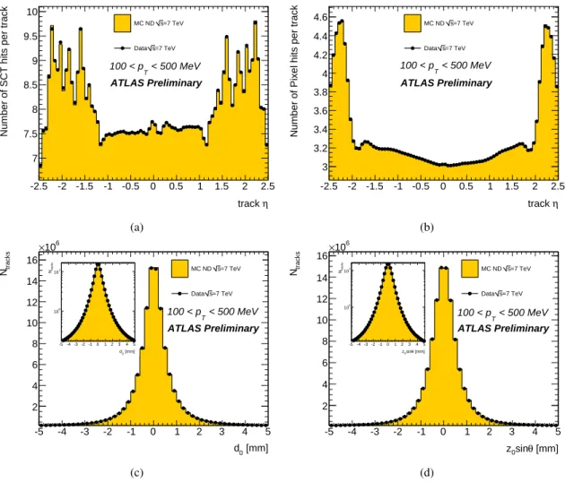
T <500 MeV here. Figure 1 shows the comparison between data and non-di
ffractive (ND) MC of those same basic track variables at 7 TeV; similar agreement is seen at 0.9 TeV. In order to remove the dependency on the physics in these plots, the p
Tspectrum of the MC is re-weighted to match that of the data. For all four variables plotted, the agreement between data and simulation is excellent and comparable to results for p
T >500 MeV.
3.2 Transverse Momentum Resolution at High p
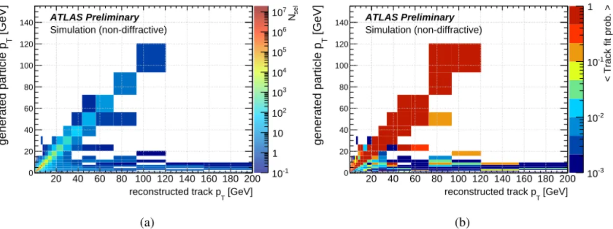
TSection 2.1 alluded to a new cut to remove mis-measured tracks. Figure 2(a) shows, in Monte Carlo, the particle p
Tversus the reconstructed track transverse momentum. This shows that while for most events the values are strongly correlated there are a number of lower p
Ttracks that are reconstructed with very high p
T. These tracks come from the non-Gaussian tails of the track momentum resolution. While these tails are small relative to the number of events in the bulk of the distribution, the p
Tspectrum is very steeply falling. Without the
χ2probability cut, these tails constitute around 30% of the tracks in the region 30
<p
T <50 GeV. We define here mis-measured tracks as those with a fractional difference in p
Trelative to the particle which is greater than 50%. As no Monte Carlo can be trusted to describe such non-Gaussian tails to such a high accuracy, it was necessary to find a cut that could remove most of such mis-measured tracks. The track fit
χ2probability of those tracks was found to be very low, as can be seen in Figure 2(b); a very loose cut at 0.01 was found to remove most mis-measured tracks in MC. Figure 3 shows, in simulation, the fraction of mis-measured tracks as a function of p
Tbefore and after this cut.
The fraction of mis-measured tracks in the highest p
Tbin used (30
<p
T <50 GeV) is reduced to 6%
after this cut. The systematic uncertainty due to the residual mis-measured tracks in data is explored in Section 4.5.
4 Analysis Procedure Overview
This section outlines the various contributions to the final corrected multiplicity distributions: the trigger,
vertex and track reconstruction efficiencies, the fraction of non-primary tracks and a new unfolding for
the track p
Tspectrum. These are all presented in the next sections where only the differences with
η track -2.5 -2 -1.5 -1 -0.5 0 0.5 1 1.5 2 2.5
Number of SCT hits per track
7 7.5 8 8.5 9 9.5 10
=7 TeV s MC ND
=7 TeV s Data
ATLAS Preliminary < 500 MeV 100 < pT
(a)
η track -2.5 -2 -1.5 -1 -0.5 0 0.5 1 1.5 2 2.5
Number of Pixel hits per track
3 3.2 3.4 3.6 3.8 4 4.2 4.4
4.6 MC ND s=7 TeV
=7 TeV s Data
ATLAS Preliminary < 500 MeV 100 < pT
(b)
[mm]
d0
-5 -4 -3 -2 -1 0 1 2 3 4 5
tracksN
2 4 6 8 10 12 14 16
106
×
=7 TeV s MC ND
=7 TeV s Data
ATLAS Preliminary < 500 MeV 100 < pT
[mm]
0 d -5 -4 -3 -2 -1012345
tracksN
106 107
(c)
[mm]
θ
0sin z
-5 -4 -3 -2 -1 0 1 2 3 4 5
tracksN
2 4 6 8 10 12 14 16
106
×
=7 TeV s MC ND
=7 TeV s Data
ATLAS Preliminary < 500 MeV 100 < pT
[mm]
θ 0sin z -5 -4 -3 -2 -1012345
tracksN
106 107
(d)
Figure 1: Comparison between data and simulation at
√s
=7 TeV for tracks between 100 and 500 MeV:
the number of silicon hits on track as a function of
ηin the SCT (a) and Pixel (b) detectors, the transverse impact parameter (c) and longitudinal impact parameters multiplied by sinθ (d). The inserts for the impact parameter plots show the log-scale plots. The p
Tdistribution of the tracks in MC is re-weighted to match the data and the number of events is scaled to the data.
respect to previous analyses are mentioned. There were no changes to the unfolding method used for the n
chspectrum so it is not described explicitly here.
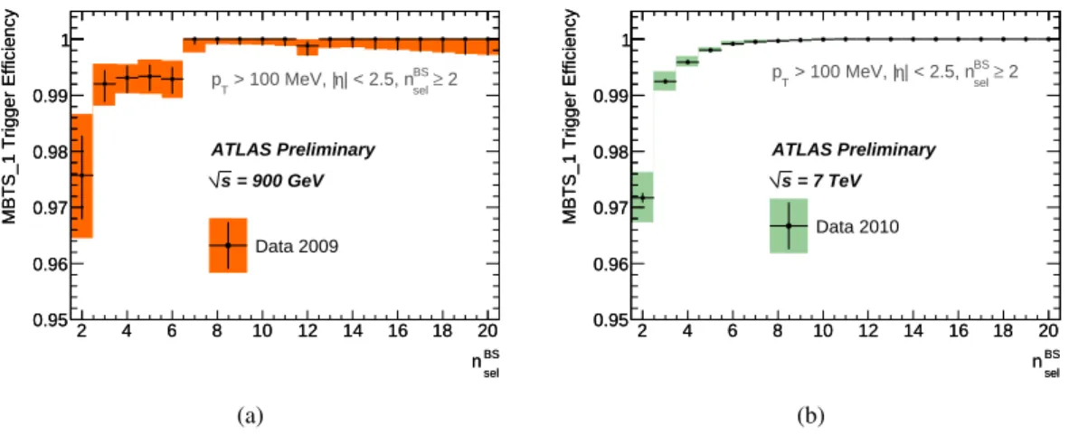
4.1 Trigger E ffi ciency
The trigger efficiency for the single-arm MBTS trigger is measured from an independent trigger in a similar way to the previous analyses. The systematic uncertainties are also derived in a similar manner.
The resulting measured trigger e
fficiency is shown in Figure 4 as a function of n
BSsel. The dependence
on other variables is again found to be negligible and is not considered further in the analysis. The
trigger e
fficiency is lower than in the previous analyses where at least one track with p
T>500 MeV was
required. This is due to the fact that events that satisfy our new selection criteria are less likely to have a
charged particle with a high enough p
Tto allow it to pass through one of the MBTS counters.
[GeV]
reconstructed track pT
20 40 60 80 100 120 140 160 180 200 [GeV] Tgenerated particle p
0 20 40 60 80 100 120 140
selN
10-1
1 10 102
103
104
105
106
107
Simulation (non-diffractive) ATLAS Preliminary
(a)
[GeV]
reconstructed track pT
20 40 60 80 100 120 140 160 180 200 [GeV] Tgenerated particle p
0 20 40 60 80 100 120 140
< Track fit prob. >
10-3
10-2
10-1
1 Simulation (non-diffractive)
ATLAS Preliminary
(b)
Figure 2: (a) MC distribution of the the particle p
Tvs the p
Tof the reconstructed tracks. The colour-scale (z-axis) indicates the number of entries, in a log-scale. Reconstructed tracks that cannot be matched to any generated particle are not displayed. (b) MC distribution of the mean track fit
χ2probability (z-axis) vs particle p
Tvs reconstructed track p
T.
[GeV]
track pT
10 20 30 40 50 60 70 80 90 100
Fraction of badly measured tracks
0 0.1 0.2 0.3 0.4 0.5 0.6 0.7 0.8 0.9
baseline cuts probability cut χ2
ATLAS Preliminary
=7 TeV s MC ND
Figure 3: Fraction of tracks as a function of the reconstructed track p
T, in simulation, where the recon-
structed p
Tdi
ffers by more than 50% from the particle p
Tbefore (black) and after (red) the track fit
χ2probability cut at 0.01. All other track selection cuts are applied.
BS
nsel
2 4 6 8 10 12 14 16 18 20
MBTS_1 Trigger Efficiency
0.95 0.96 0.97 0.98 0.99 1
≥ 2
BS
| < 2.5, nsel
η > 100 MeV, | pT
ATLAS Preliminary
BS
nsel
2 4 6 8 10 12 14 16 18 20
MBTS_1 Trigger Efficiency
0.95 0.96 0.97 0.98 0.99 1
Data 2009 = 900 GeV s
(a)
BS
nsel
2 4 6 8 10 12 14 16 18 20
MBTS_1 Trigger Efficiency
0.95 0.96 0.97 0.98 0.99 1
BS
nsel
2 4 6 8 10 12 14 16 18 20
MBTS_1 Trigger Efficiency
0.95 0.96 0.97 0.98 0.99 1
Data 2010 ATLAS Preliminary
= 7 TeV s
≥ 2
BS
| < 2.5, nsel
η > 100 MeV, | pT
(b)
Figure 4: Trigger efficiency as a function of n
BSselat 0.9 (a) and 7 TeV (b). The coloured error bands show the total uncertainty, the black vertical lines the statistical uncertainty of the events collected with the independent trigger.
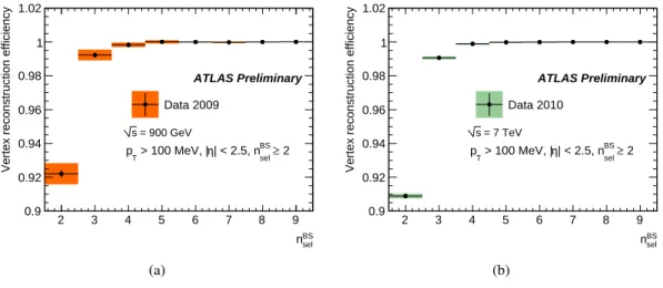
4.2 Vertex Reconstruction E ffi ciency
The method used to extract the vertex reconstruction efficiency is maintained with respect to the previous analyses; we look at the events that pass our modified event selection, where the tracks are defined with respect to the BS parameters, and measure the fraction of those events that have a reconstructed vertex. The efficiency is measured in bins of n
BSsel. The beam backgrounds are explicitly removed before calculating this ratio. An inefficiency is observed for vertices with two tracks in our phase space due to the track selection in the vertex reconstruction algorithm being tighter than the cuts for the analysis. For vertices with more than two tracks, the parametrisation with respect to only n
BSsel, shown in Figure 5, was found to be sufficient. For events with only two tracks, the reconstruction efficiency was found to depend on the projection along the beam axis of the separation between the two tracks,
∆z
BS0, when the tracks are extrapolated to the beam spot. Moreover, this parametrisation was found to depend on the p
Tof the tracks. The parametrisation, shown in Figure 6, in terms of
∆z
BS0is thus done for two bins, p
minT <200 and p
minT >200 MeV, where p
minTis the lowest p
Tof the two tracks.
The systematic uncertainties considered for the vertex reconstruction algorithm come from the re- moval or not of the beam background contribution. The efficiency without removing the beam back- ground contribution is calculated and the di
fference with respect to the nominal is taken as a systematic error.
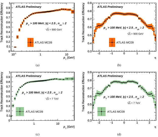
4.3 Track Reconstruction E ffi ciency
The track reconstruction efficiency is determined, as in the previous iterations, from simulation. Ex- tensive comparisons between data and simulation are performed to establish that the simulation of the silicon detectors describes the data to high accuracy. The track reconstruction e
fficiency is binned in p
Tand
η; its projection onto those two variables is shown in Figure 7. The difference in the track recon-struction e
fficiencies between the two energies is dominated by the di
fferent number and configuration
of the disabled Pixel and SCT modules in the 2009 data and in the 2010 run; there were fewer disabled
modules in the 2010 run.
BS
nsel
2 3 4 5 6 7 8 9
Vertex reconstruction efficiency
0.9 0.92 0.94 0.96 0.98 1 1.02
Data 2009
ATLAS Preliminary
= 900 GeV s
≥ 2
BS
| < 2.5, nsel
η > 100 MeV, | pT
(a)
BS
nsel
2 3 4 5 6 7 8 9
Vertex reconstruction efficiency
0.9 0.92 0.94 0.96 0.98 1 1.02
Data 2010
ATLAS Preliminary
= 7 TeV s
≥ 2
BS
| < 2.5, nsel
η > 100 MeV, | pT
(b)
Figure 5: Vertex reconstruction e
fficiency as a function of n
BSselat 0.9 (a) and 7 TeV (b). The coloured error bands show the total uncertainty, the black vertical lines the statistical uncertainty.
[mm]
BS
z0
∆
0 5 10 15 20 25 30 35 40 45
Vertex reconstruction efficiency
0 0.2 0.4 0.6 0.8 1 1.2
= 900 GeV s
Data 2009,
ATLAS Preliminary < 200 MeV
min
= 2, 100 MeV < pT BS
nsel
| < 2.5 η
|
(a)
[mm]
BS
z0
∆
0 5 10 15 20 25 30 35 40
Vertex reconstruction efficiency
0 0.2 0.4 0.6 0.8 1 1.2
= 900 GeV s
Data 2009,
ATLAS Preliminary
| < 2.5 η > 200 MeV, |
min
= 2, pT BS
nsel
(b)
[mm]
BS
z0
∆
0 10 20 30 40 50 60 70
Vertex reconstruction efficiency
0 0.2 0.4 0.6 0.8 1 1.2
= 7 TeV s Data 2010,
ATLAS Preliminary < 200 MeV
min
= 2, 100 MeV < pT BS
nsel
| < 2.5 η
|
(c)
[mm]
BS
z0
∆
0 10 20 30 40 50 60 70
Vertex reconstruction efficiency
0 0.2 0.4 0.6 0.8 1 1.2
= 7 TeV s Data 2010,
ATLAS Preliminary
| < 2.5 η > 200 MeV, |
min
= 2, pT BS
nsel
(d)
Figure 6: Vertex reconstruction e
fficiency at 0.9 TeV (a,b) and 7 TeV (c,d) for n
BSsel =2 vs
∆z
BS0for events
where the lowest track p
Tis below (a,c) and above (b,d) 200 MeV .
[GeV]
pT
10-1 1 10
Track Reconstruction Efficiency
0 0.1 0.2 0.3 0.4 0.5 0.6 0.7 0.8 0.9 1
ATLAS Preliminary
≥ 2
| < 2.5 , nch
η > 100 MeV, | pT
= 900 GeV s
ATLAS MC09
[GeV]
pT
10-1 1 10
Track Reconstruction Efficiency
0 0.1 0.2 0.3 0.4 0.5 0.6 0.7 0.8 0.9 1
(a)
η
-2 -1 0 1 2
Track Reconstruction Efficiency
0.3 0.4 0.5 0.6 0.7 0.8 0.9
ATLAS Preliminary
≥ 2
| < 2.5 , nch
η > 100 MeV, | pT
= 900 GeV s
ATLAS MC09
η
-2 -1 0 1 2
Track Reconstruction Efficiency
0.3 0.4 0.5 0.6 0.7 0.8 0.9
(b)
[GeV]
pT
1 10
Track Reconstruction Efficiency
0 0.1 0.2 0.3 0.4 0.5 0.6 0.7 0.8 0.9 1
ATLAS Preliminary
≥ 2
| < 2.5 , nch
η > 100 MeV, | pT
= 7 TeV s
ATLAS MC09
[GeV]
pT
1 10
Track Reconstruction Efficiency
0 0.1 0.2 0.3 0.4 0.5 0.6 0.7 0.8 0.9 1
(c)
η
-2 -1 0 1 2
Track Reconstruction Efficiency
0.3 0.4 0.5 0.6 0.7 0.8 0.9
ATLAS Preliminary
≥ 2
| < 2.5 , nch
η > 100 MeV, | pT
= 7 TeV s
ATLAS MC09
η
-2 -1 0 1 2
Track Reconstruction Efficiency
0.3 0.4 0.5 0.6 0.7 0.8 0.9
(d)
Figure 7: Track reconstruction e
fficiency as a function of p
T(a,c) and
η(b,d) for
√s
=0.9 TeV (a,b) and 7 TeV (c,d). The total uncertainties on each point are shown as coloured bands, the vertical error bars represent the statistical uncertainty of the Monte Carlo.
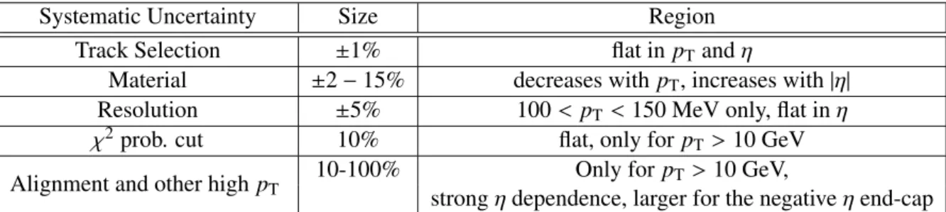
4.3.1 Systematic Uncertainties on the Track Reconstruction Efficiency
The summary of the systematic uncertainties on the track reconstruction e
fficiencies is shown in Table 1.
The track reconstruction efficiency systematic uncertainties are taken to be the same at both energies but are derived from studies done with the 7 TeV data and MC. The dominant systematic uncertainty is the material uncertainty which becomes large at high
ηand low p
T.
Material Uncertainty
Two di
fferent data driven methods are used to estimate the di
fference between the real detector and the material description in the simulation; the first reconstructs the invariant mass of the K
0sdecaying to two charged pions; the second is based on comparing the track lengths in data and simulation. The K
s0has greatest sensitivity to small radii, while the track length study probes the material description in the simulation in terms of nuclear interaction length (λ), starting after the Pixel detector.
Thus, the combination of both methods provides good sensitivity to the full Inner Detector.
The K
0smethod is similar to that used in [2] but uses significantly more data. The reconstructed mass
is measured as a function of
η,φand decay radius. The data is compared to the distributions obtained
with the nominal simulation as well as with a simulation in which the non-active material in the Inner
Systematic Uncertainty Size Region
Track Selection
±1%flat in p
Tand
ηMaterial
±2−15% decreases with p
T, increases with
|η|Resolution
±5%100
<p
T <150 MeV only, flat in
ηχ2
prob. cut 10% flat, only for p
T>10 GeV
Alignment and other high p
T10-100% Only for p
T >10 GeV,
strong
ηdependence, larger for the negative
ηend-cap Table 1: The systematic uncertainties on the tracking e
fficiency. All uncertainties are quoted relative to the track reconstruction e
fficiency.
+) π η (
-2.5 -2 -1.5 -1 -0.5 0 0.5 1 1.5 2 2.5
fitted mass ratio0 SK
0.997 0.998 0.999 1 1.001 1.002 1.003
Data 2010 / MC ND (nominal) MC ND (+5%) / MC ND (nominal) MC ND (+10%) / MC ND (nominal)
= 7 TeV s ATLAS Preliminary
(a)
-) π η (
-2.5 -2 -1.5 -1 -0.5 0 0.5 1 1.5 2 2.5
fitted mass ratio0 SK
0.997 0.998 0.999 1 1.001 1.002 1.003
Data 2010 / MC ND (nominal) MC ND (+5%) / MC ND (nominal) MC ND (+10%) / MC ND (nominal)
= 7 TeV s ATLAS Preliminary
(b)
Figure 8: Fitted K
s0mass ratios as a function of
ηfor data and various MC simulated material descriptions over to the nominal MC sample. The
ηvalues are obtained from the positive (a) and negative (b) track.
The K
s0candidates considered for these plots are required to have a reconstructed decay radius smaller than 25 mm, i.e. before the beam pipe. Furthermore, the two pion tracks of all K
s0candidates are required to have at least four silicon hits. The vertical error bars show the statistical uncertainty only (data and MC), while the horizontal orange bands indicate the uncertainty due to the magnetic field strength.
Detector has been increased by 10%, both in terms of radiation length and interaction length. The mass versus
ηis shown in figure 8. From this study, one can see that the material description in the nominal MC sample models the observed masses in the barrel (|η|
.1.3) well; one can conclude that in the region probed by this study, 10% is a good estimate for the possible amount of extra material present in the detector relative to the MC.
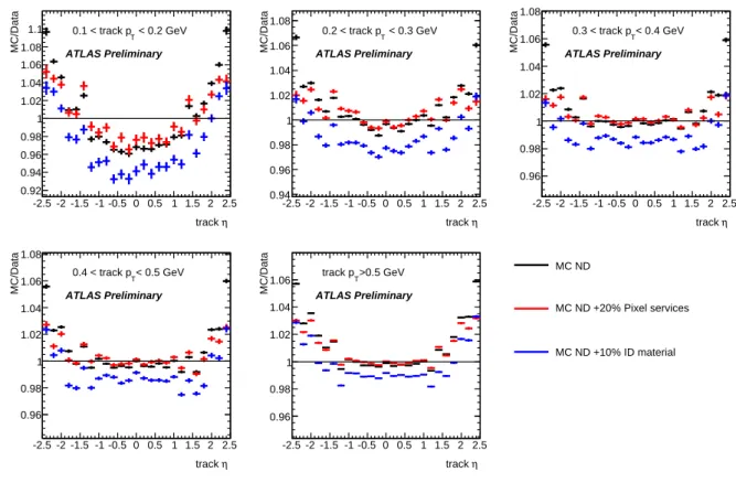
The track length method is also similar to that used in [2]; tracks are reconstructed using the Pixel detector only and are matched to our good tracks that have the full track selection cuts applied. The fraction of Pixel only tracks with a successful match to a full track defines the SCT extension rate.
This rate is compared between data and Monte Carlo simulation; some example regions are shown in
Figure 9. We compare to the nominal simulation, the additional 10% ID material sample and another
sample where only the external Pixel services are scaled by 20%. For this study the p
Tspectrum of
the Monte Carlo is re-weighted to reproduce the observed spectrum. The barrel region (|η|
<1.3) again
shows good agreement with the nominal Monte Carlo with small deviations observed in the lowest p
Tslice (100-200 MeV). The data in the region below
|η|of 2.0 agrees better with the nominal sample than
with the 10% enhanced material sample. The end-cap regions (|η|
>2.0) show deviations, in all p
Tslices, that are not covered by the 10% enhanced material sample. In this di
fficult detector region the
η track -2.5 -2 -1.5 -1 -0.5 0 0.5 1 1.5 2 2.5
MC/Data
0.92 0.94 0.96 0.98 1 1.02 1.04 1.06 1.08
1.1 < 0.2 GeV
0.1 < track pT
ATLAS Preliminary
η track -2.5 -2 -1.5 -1 -0.5 0 0.5 1 1.5 2 2.5
MC/Data
0.94 0.96 0.98 1 1.02 1.04 1.06 1.08
< 0.3 GeV 0.2 < track pT
ATLAS Preliminary
η track -2.5 -2 -1.5 -1 -0.5 0 0.5 1 1.5 2 2.5
MC/Data
0.96 0.98 1 1.02 1.04 1.06 1.08
< 0.4 GeV 0.3 < track pT
ATLAS Preliminary
η track -2.5 -2 -1.5 -1 -0.5 0 0.5 1 1.5 2 2.5
MC/Data
0.96 0.98 1 1.02 1.04 1.06 1.08
< 0.5 GeV 0.4 < track pT
ATLAS Preliminary
η track -2.5 -2 -1.5 -1 -0.5 0 0.5 1 1.5 2 2.5
MC/Data
0.96 0.98 1 1.02 1.04
1.06 >0.5 GeV
track pT
ATLAS Preliminary
MC ND
MC ND +20% Pixel services
MC ND +10% ID material
Figure 9: Ratio of the MC over data of the SCT extension rate in slices of p
Tand as a function of
η, forthe nominal MC (black) as well as the sample with 10% extra material in the ID (blue) and the sample with 20% more material in the external Pixel services (red). The horizontal black line at unity is to guide the eye.
service structures (cooling pipes, cables, etc.) of the Pixel detector are the most likely place where the MC material description is not accurate. The 20% enhanced Pixel service material and 10% enhanced ID material samples have a similarly strong e
ffect on the SCT extension rate in these most forward regions.
Two slightly different approaches have been used to determine the final material uncertainty on the track reconstruction e
fficiency. The first combines the uncertainty due to the 10% increased material sample with the full di
fference between data and simulation of the SCT extension rate; the second com- bines the uncertainties of the 10% increased material sample with that of the 20% increased Pixel services sample. These two methods yield very similar uncertainties for most bins in p
Tand
η. For the bins wherethe methods di
ffer, the most conservative number is considered. The total uncertainty due to the material goes from 8% at low p
Tdown to 2% above 500 MeV for the barrel region; it increases with
ηwith the largest uncertainties being for 2.3
<|η|<2.5 which is 15% in the first p
Tbin and 7% above 500 MeV.
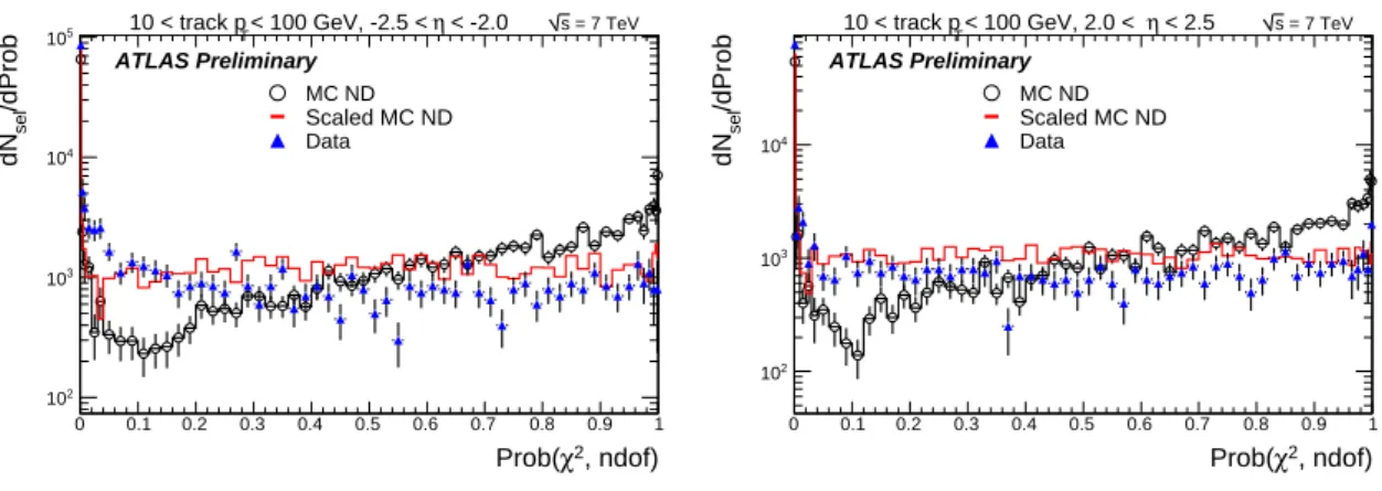
Uncertainty due to theχ2Probability Cut
The track-fit probability has been shown, Figure 2(b), to
offer powerful discrimination against the badly measured tracks. Unfortunately, the distribution of this
variable is not well modelled in the MC. The differences between data and MC in the
χ2probability
distributions are caused by di
fferences either in the number of degrees-of-freedom or in the
χ2distribu-
tions. Figure 10 shows, for one particular
|η|region, the
χ2probability distribution in data compared to
MC. From studies, we find that the number of degrees-of-freedom is in reasonably good agreement for
the end-cap, while a clear shift is seen in the barrel; the
χ2is smaller in MC than in data. The track-fit
, ndof) χ2
Prob(
0 0.1 0.2 0.3 0.4 0.5 0.6 0.7 0.8 0.9 1
/dProbseldN
102
103
104
105 < 100 GeV, -2.5 <η < -2.0
10 < track pT s = 7 TeV
MC ND Scaled MC ND Data ATLAS Preliminary
, ndof) χ2
Prob(
0 0.1 0.2 0.3 0.4 0.5 0.6 0.7 0.8 0.9 1
/dProbseldN
102
103
104
< 2.5 η < 100 GeV, 2.0 <
10 < track pT s = 7 TeV
MC ND Scaled MC ND Data ATLAS Preliminary
Figure 10: Comparison of track-fit probability for
−2.5< η <−2.0 (left) and 2.0< η <2.5 (right) . All plots are for a reconstructed track p
Tabove 10 GeV. The blue filled triangles show the data, while the black histogram indicates the MC (normalised to the number of data entries). The red histogram shows the MC with a scale factor of 1.3 applied to the
χ2.
[GeV]
track pT
10 15 20 25 30 35 40 45 50
prob-cut2χwithout /NTrkprob-cut2χwith NTrk
0 0.2 0.4 0.6 0.8 1
=7 TeV s MC ND
=7 TeV s Data
ATLAS Preliminary
Figure 11: Fraction of tracks in data (black) and in MC (red) that pass the
χ2probability cut of 0.01 as a function of the reconstructed track p
T. The cut is only applied for tracks with p
T >10 GeV.
probability distributions are not flat, as one would expect in a
χ2-fit with correct Gaussian errors.
In order to get a better agreement with the data, a scaling factor is introduced to increase the
χ2values of the tracks in the MC. Figure 10 shows in red the distribution after the error scaling is applied;
this shows that after error scaling the distribution in MC models the data significantly better.
Figure 11 shows the fraction of tracks in data and in MC that pass the
χ2probability cut at 0.01 as a function of the reconstructed track p
T. The fraction is 1 for tracks below 10 GeV where the cut is not applied. The maximum difference between data and MC is found to be 10%, which is taken as a conservative estimate of the systematic uncertainty due to this cut. The uncertainty is taken to be flat in
p
T.
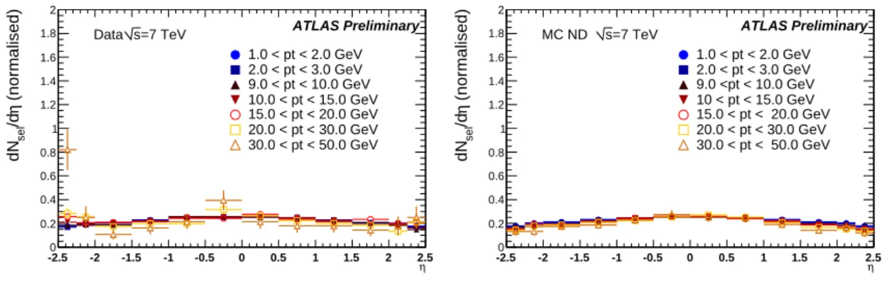
Alignment and Other High-pT Effects
Despite the
χ2probability cut, some mis-measured tracks
remain in our data sample. In MC we expect the fraction of bad tracks in the bin from 30-50 GeV to be
roughly 6% of the total number of tracks. By looking at the distribution of the
ηdistribution of the tracks
in p
Tbins, one sees strong indications that there are significantly more mis-measured tracks in data than
-2.5 -2 -1.5 -1 -0.5 0 0.5 1 1.5 2 2.5η
(normalised)η/dseldN
0 0.2 0.4 0.6 0.8 1 1.2 1.4 1.6 1.8 2
1.0 < pt < 2.0 GeV 2.0 < pt < 3.0 GeV 9.0 < pt < 10.0 GeV 10.0 < pt < 15.0 GeV 15.0 < pt < 20.0 GeV 20.0 < pt < 30.0 GeV 30.0 < pt < 50.0 GeV
=7 TeV s
Data ATLAS Preliminary
-2.5 -2 -1.5 -1 -0.5 0 0.5 1 1.5 2 2.5η
(normalised)η/dseldN
0 0.2 0.4 0.6 0.8 1 1.2 1.4 1.6 1.8 2
1.0 < pt < 2.0 GeV 2.0 < pt < 3.0 GeV 9.0 <pt < 10.0 GeV 10 < pt < 15.0 GeV 15.0 < pt < 20.0 GeV 20.0 < pt < 30.0 GeV 30.0 < pt < 50.0 GeV
=7 TeV s
MC ND ATLAS Preliminary
Figure 12:
ηdistribution in data (left) and MC (right) in di
fferent bins in p
T. In MC there seems to be very little variation with p
T. In data the variations are used to estimate the uncertainty due to residual mis-alignment and other sources of mis-measured tracks. The different p
Tbins are normalised such that the integral
−1.0< η <1.0 is the same.
in MC even after this cut. Figure 12 shows the
ηdistribution in bins of p
Tfor data (left) and MC (right).
Only tracks above 1 GeV are considered in this study. In MC one sees there is no noticeable variation of the shape as a function of p
T. In data large variations are seen, in particular in the lowest and highest bins in
η. The effect on the negative
ηend-cap is more pronounced than on positive
ηend-cap. There is a known problem with the alignment in negative
ηend-cap in the data re-processing used for this analysis.
By taking the most conservative approach that there should be no dependency on p
Tof the
ηspectrum, one can estimate the systematic uncertainty in each bin in p
Tand
ηdue to non-modelled detector e
ffects.
We consider the tracks between 1 and 3 GeV as the control distribution; any deviation from this is taken as a systematic uncertainty. This systematic uncertainty is found to be consistent with zero for tracks below 10 GeV. The largest systematic uncertainty is for 30
<p
T <50 GeV and
−2.5< η <−2.25 wherethe systematic uncertainty is 100%.
Track Selection Uncertainty
The track selection uncertainty is determined by removing, or in the case of the impact parameter cuts widening to 2.5 mm, each of the track selection cuts one at a time and comparing the distributions between data and Monte Carlo; any di
fference is taken as a systematic uncertainty. The total uncertainty on the track selection is determined by adding each of these sources in quadrature. The uncertainty is found to be 1% at high
η, but for the sake of simplicity this uncertainty isconsidered to be a constant 1%.
Resolution Uncertainty
The applied minimum momentum requirement at various stages of the pattern recognition inside the track reconstruction algorithm introduces an inefficiency due to the momentum resolution. A significantly worse momentum resolution or a significant bias in the momentum estimation in data compared to MC can result in a change in the migration out of the first bin in p
T(100
<p
T <150 MeV). The track resolution at the seed finding stage in Monte Carlo was increased by a very
conservative 10 MeV, making the p
Tresolution e
ffectively 15 MeV instead of 10 MeV. The e
ffect of this
shift on the track reconstruction e
fficiency in the first p
Tbin was found to be about 5%.
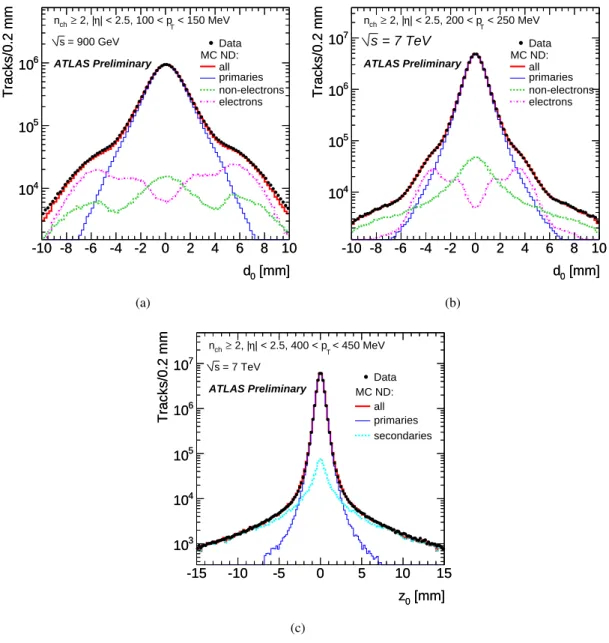
4.4 Estimation of the Fraction of Tracks Originating from Non-Primary Particles The method previously used to obtain the fraction of secondary tracks in data by using a fit to the tails of the d
0distribution is applied in this analysis to all non-primary tracks; a distinction is no longer made between secondary and fake tracks. Above 500 MeV the contribution from photon conversions to a pair of electrons is small, but this is no longer the case at lower p
T. We now fit separately for primaries, non- primaries from electrons and other non-primaries. The electron contribution dominates at larges values of d
0whereas the other non-primaries dominate under the peak. The layer-0 hit requirement removes a large fraction of the electrons in the tails of the distributions, which allows the fit to all three parameters to be performed on the data.
A separate fit was carried out in eight bins of 50 MeV for 100
<p
T <500 MeV with an additional single fit for p
T >500 MeV. For this last bin, there is no need to separate electrons from other non- primaries as the electron contribution is very low in both the tails and the peak.
These results are cross-checked by fitting the z
0distribution and the difference with respect to the fit to d
0is taken as a systematic uncertainty. For the fit to z
0, no distinction is made between non-primaries from electrons and non-electrons. The second contribution to the systematic uncertainty is due to the variation of the d
0region used for the fit.
Figure 13 shows examples of the the d
0distributions at
√s
=0.9 TeV (a) and
√s
=7 TeV (b) and the z
0distribution at
√s
=7 TeV (c) for the data and di
fferent components of the MC. The bumps in the d
0distributions at low p
Tin the secondaries are due to interactions with the beam pipe and the first pixel layer.
4.5 Unfolding the p
TDistribution
To fully account for and correct for the bin migration in p
Tof poorly-reconstructed tracks, an iterative unfolding method is applied on the corrected, reconstructed- p
Tdistribution after applying all the other corrections [4]. This method is similar to that implemented for the n
chunfolding. Appendix D describes this procedure in more detail. The e
ffect on the p
Tspectrum in data due to this new unfolding procedure is at most 10% at
√s
=0.9 TeV and 3% at
√s
=7 TeV.
4.5.1 Systematic Uncertainties on the
p
TUnfoldingThe iterative unfolding procedure is designed to be minimally dependent on the input spectrum used to fill the matrix. The nominal values are taken where for the first iteration the input spectrum is that of the MC; the results converge after 3 iterations
3. To estimate any residual effect due to the input spectrum at the first iteration, we assume a flat p
Tspectrum and take the di
fference between the final distributions as a systematic uncertainty. With a flat initial probability distribution, the unfolding converges after 6 iterations at 7 TeV and 5 at 0.9 TeV. The difference with respect to the nominal input distribution is found to be 4% or less for all bins. A similar di
fference is observed when using an exponential as the initial probability distribution.
4.6 Closure Test
The closure test exercise has been used in the previous analyses to demonstrate the performance of the corrections and Bayesian unfolding. The nominal MC samples were reconstructed and corrected back to the particle-level using the same procedure as applied to data. The corrected particle-level distributions were then compared to the initial known particle-level distributions from
pythia. We found a difference3Convergence is defined as the first iteration in which theχ2 difference between the result of the unfolding and the input distribution for that iteration is less than the number of bins.
[mm]
d0
-10 -8 -6 -4 -2 0 2 4 6 8 10
Tracks/0.2 mm
104
105
106
electrons non-electrons primaries all MC ND:
Data < 150 MeV
| < 2.5, 100 < pT
η 2, |
ch≥ n
= 900 GeV s
ATLAS Preliminary
[mm]
d0
-10 -8 -6 -4 -2 0 2 4 6 8 10
Tracks/0.2 mm
104
105
106
(a)
[mm]
d0
-10 -8 -6 -4 -2 0 2 4 6 8 10
Tracks/0.2 mm
104
105
106
107
electrons non-electrons primaries all MC ND:
Data < 250 MeV
| < 2.5, 200 < pT
η 2, |
ch≥ n
= 7 TeV s
ATLAS Preliminary
[mm]
d0
-10 -8 -6 -4 -2 0 2 4 6 8 10
Tracks/0.2 mm
104
105
106
107
(b)
[mm]
z0
-15 -10 -5 0 5 10 15
Tracks/0.2 mm
103
104
105
106
107
secondaries primaries all MC ND:
Data < 450 MeV
| < 2.5, 400 < pT
η 2, |
ch≥ n
= 7 TeV s
ATLAS Preliminary
[mm]
z0
-15 -10 -5 0 5 10 15
Tracks/0.2 mm
103
104
105
106
107
(c)
Figure 13: d
0distribution for primary (blue) and non-primary particles after scaling them to the best fit value for p
T =100
−150 MeV at
√s
=0.9 TeV (a) and p
T =200
−250 MeV at
√s
=7 TeV (b).
The non-primary particles are split into electrons (pink) coming mostly from photon conversions and non-electrons (green) which are the dominant contribution after the analysis cuts are applied. (c) shows the fit to the z
0distribution at
√s
=7 TeV in the range p
T =450
−500 MeV; the non-primaries are
shown as pale blue lines.
of 1.5% between the generated and corrected particle-level distributions in the second bin (n
ch =3) of the n
chdistribution. In all other bins the corrections and unfolding reproduce the original particle-level dis- tributions. The agreement of the charged-particle multiplicity spectrum as a function of pseudorapidity and the average p
Tvs n
chis at the level of 1% in all bins.
5 Results
5.1 Total Uncertainties
The various uncertainties are propagated through the entire analysis by fluctuating the correction factors up and down by their uncertainties; the resulting di
fference on the unfolded distribution is taken as a systematic error. All sources of uncertainty are assumed to be un-correlated. Any correlations between the number of events in the denominator and the distribution in the numerator are thus automatically taken into account. The statistical errors are shown in all plots as vertical error bars, the total uncertainties as coloured bands.
For the sake of illustration, the summary of the systematic uncertainties considered for this analysis are shown in Table 2 for both
√s
=0.9 TeV and
√s
=7 TeV separated out into the components that a
ffect the number of events and those that a
ffect the
ηdistribution. The largest systematic uncertainties come from the measurement of the track reconstruction efficiency.
Systematic uncertainty on the number of events,Nev
√
s
=0.9 TeV
√s
=7 TeV
Trigger e
fficiency 0.2% 0.2%
Vertex-reconstruction efficiency
<0.1%
<0.1%
Track-reconstruction e
fficiency 1.0% 0.7%
Different Monte Carlo tunes 0.4% 0.4%
Total uncertainty on N
ev1.1% 0.8%
Systematic uncertainty on (1/Nev)·(dNch/dη) atη=0
Track-reconstruction efficiency 3.1% 3.1%
Trigger and vertex e
fficiency
<0.1%
<0.1%
Secondary fraction 0.4% 0.4%
Total uncertainty on N
ev −1.1% −0.8%Total uncertainty on (1/N
ev)·(dN
ch/dη) atη=0 2.1% 2.3%
Table 2: Summary of systematic uncertainties on the number of events, N
ev, and on the charged-particle density (1/N
ev)·(dN
ch/dη) atη=0. All sources of uncertainty are assumed to be uncorrelated.
5.2 Final Plots
The corrected distributions of primary charged particles for
√s
=0.9 TeV with p
T >100 MeV and
|η|<