ATLAS NOTE ATLAS-CONF-2014-046

ATLAS-CONF-2014-046 06July2014

ATLAS NOTE

ATLAS-CONF-2014-046

July 3, 2014

Calibration of the performance of b-tagging for c and light-flavour jets in the 2012 ATLAS data

The ATLAS Collaboration

Abstract

A variety of algorithms have been developed, within the ATLAS experiment at the Large Hadron Collider, to distinguishb-quark jets from jets containing only lighter quarks. This note describes measurements of the efficiency of the most performant of these b-tagging algorithms, as carried out on the data collected at √

s = 8 TeV in 2012, for charm and light-flavour jets. The results, which correct the efficiency in simulation to that measured in data, are presented in the form of jet transverse momentum dependent (and in the case of the light-flavour jets, pseudorapidity dependent) scale factors. Compared to previous calibration analyses, improvements have been made driven by the larger dataset collected in 2012, as well as by a refinement of the existing analyses. These results complement those obtained forbjets as presented in a previous note.

⃝c Copyright 2014 CERN for the benefit of the ATLAS Collaboration.

Reproduction of this article or parts of it is allowed as specified in the CC-BY-3.0 license.

1 Introduction

This note describes the methods used to calibrate the performance of theb-tagging algorithms used by the ATLAS experiment [1] at the Large Hadron Collider. As an example, it discusses the results obtained for the so-called MV1 algorithm, which is used in many physics analyses carried out in the experiment.

The performance ofb-tagging algorithms is characterised by the efficiency of tagging abjet,ϵb, and the probabilities of mistakenly tagging as abjet a jet originating from a cquark, ϵc, or a light-flavour parton,ϵl. Here, “light-flavour” partons areu,d,squarks or gluonsg; the resulting efficiency is referred to as the “mistag rate”. For each b-tagging algorithm, working points are defined as a function of the averageb-jet efficiency as measured in simulation.

The efficienciesϵb,ϵcand the mistag rateϵlare measured on data. The calibration results are provided as data/MC efficiency scale factors, e.g.,κ^datac ^/sim ≡ ϵc^data/ϵc^sim and similarly forband light-flavour jets.

The calibration of the performance forbjets has been described in a separate note [2]; this note describes the corresponding performance calibrations forcand light-flavour jets.

This note is subdivided as follows: Section 2 describes the samples and object selections used for the calibration measurements, as well as the object reconstruction, calibration, and correction procedures.

Section 3 provides a description of the MV1 tagging algorithm and of the strategy used to calibrate its performance. Thec-jet tagging efficiency is measured in an inclusive sample of jets with associatedD^∗ mesons, as described in Section 4. The mistag rate is measured in an inclusive jet sample, as detailed in Section 5. Section 6 concludes this note.

2 Data and simulation samples, object selection

The studies presented in this note are based on a data sample corresponding to 20.3 fb⁻¹of 8 TeV proton- proton collision data collected by the ATLAS experiment during 2012. The triggers used to collect the data for the specific studies are described in the corresponding sections.

The key objects forb-tagging are the jets reconstructed from the energy deposits measured in the calorimeter, the tracks reconstructed in the inner detector, and the selected primary vertex. The tracks are associated with the calorimeter jets based on their angular distance¹ ∆R ≡ √

∆η²+ ∆ϕ². The track selection criteria depend on theb-tagging algorithm, and are detailed in Refs. [3, 4].

Jets are reconstructed from topological clusters [5] formed from energy deposits in the calorimeter using the anti-k_t algorithm with a radius parameter of 0.4 [6–8]. Two approaches towards jet clustering are employed by ATLAS: one starting from energy clusters calibrated at the electromagnetic scale (“EM jets”), and one starting from clusters calibrated using the local cluster weighting (LCW) method (“LC jets”). The measured jet energies are corrected using the jet area method [9, 10] to reduce effects due to additional proton-proton interactions in the same or neighbouring bunch crossings, referred to as pile-up in the following. The results shown in this note will pertain to LC jets; the procedure and results obtained for EM jets are very similar.

Jets are calibrated using a transverse momentum, p_T, andηdependent simulation-based calibration scheme independent of quark flavour, with in situ corrections based on data. Only jets withpT >20 GeV and |η| < 2.5 are in general used for b-tagging in physics analyses. To reduce the contribution from jets arising from pile-up, jets with p_T < 50 GeV and|η| < 2.4 are required to satisfy JVF> 0.5, where JVF is the “jet vertex fraction”, i.e., the ratio of the sum of the pT of tracks associated with the jet and also associated with the primary vertex, to the sum of pT of all tracks associated with the jet. The

1ATLAS uses a right-handed coordinate system with its origin at the nominal interaction point in the centre of the detector, and thezaxis along the beam line. Thexaxis points to the centre of the LHC ring, and theyaxis points upwards. Cylindrical coordinates (r, ϕ) are used in the transverse plane, withϕbeing the azimuthal angle around the beam line. The pseudorapidity ηis defined in terms of the polar angleθasη=−ln tan(θ/2).

measurement of the jet energy, the jet energy scale determination and the specific cuts used to reject jets of bad quality are described in Ref. [11].

Several Monte Carlo (MC) simulated samples are used throughout this note. To reproduce the pile-up conditions in the data, minimum bias interactions generated with Pythia8 [12] have been superimposed on the simulated events. To simulate the detector response, the generated events are processed through a GEANT4 [13] simulation of the ATLAS detector, and then reconstructed and analysed in the same way as the data. The simulated detector geometry corresponds to a perfectly aligned inner detector and the ma- jority of its disabled pixel modules and front-end chips seen in data are masked in the simulation. Some samples employed for the evaluation of systematic uncertainties use a fast simulation instead, where the interactions in the calorimeters are simulated using parametrised functions. The ATLAS simulation infrastructure is described in more detail elsewhere [14].

To bring the simulation into agreement with data for distributions where discrepancies are known to be present, corrections have been applied to simulated samples. The distribution of the average number of interactions per bunch crossing (⟨µ⟩) has been reweighted to ensure good agreement in the number of reconstructed primary vertices between data and simulation.

The labelling of the flavour of a jet in simulation is done by spatially matching the jet with generator level partons: if abquark (after final-state radiation) is found within∆R < 0.3 of the jet direction, the jet is labelled as abjet. If nobquark is found the procedure is repeated forcquarks. A jet for which no such association can be made is labelled as a light-flavour jet.

3 Taggers and working points

Several algorithms to identifybjets have been developed. They range from relatively simple algorithms based on impact parameter (IP3D) and secondary vertex (SV1) to the more refined JetFitter algorithm, which exploits the topology of weakb- andc-hadron decays, using a Kalman filter to search for a com- mon line connecting the primary vertex to beauty and charm decay vertices. These algorithms are docu- mented in Ref. [4].

The most discriminating variables resulting from these algorithms are combined in artificial neural networks, and output weight probability densities evaluated separately for b, c, and light-flavour jets.

The MV1 algorithm employs an artifical neural network based on IP3D, SV1 and JetFitter. It is trained withbjets as signal and light-flavour jets as background, and computes atag weightfor each jet.

The calibrations described in this note apply to cases where fixed cuts are applied to the tag weight distribution. These fixed cuts orworking pointsare generally tuned to obtain specifiedb-jet efficiencies intt¯samples (for jets satisfyingpT > 20 GeV and|η| <2.5). Fig. 1 shows the performance of the MV1 tagging algorithm evaluated under these conditions for at¯tsample produced using Powheginterfaced to Pythia6 [15] with the Perugia 2011C tune [16], and CT10 parton density functions (PDFs) [17].

The performance of the MV1 algorithm has been calibrated at working points corresponding to efficiencies of 60%, 70% and 80%. The results shown in this note are for the 70% nominalb-jet efficiency working point; calibration results obtained for other working points are generally similar. The efficiency of the MV1 algorithm to tagb,c, and light-flavour jets asbjets, for this working point, is shown in Fig. 2 as a function of jetp_Tand|η|, again for simulatedtt¯events.

4 c-jet e ffi ciency calibration: D

method

The efficiency with which ab-tagging algorithm tagscjets is referred to as thec-jet tagging efficiency.

This efficiency is measured using a sample of jets containingD^∗+mesons (where charge-conjugate de- cays are implicitly included), by comparing the yield of D^∗+ mesons before and after the tagging re- quirement. The D^∗+ → D⁰π⁺ decay mode offers distinctive kinematic features, resulting in a modest

b-jet efficiency

0.55 0.6 0.65 0.7 0.75 0.8 0.85 0.9

Light-flavour jet rejection rate

1 10 102

103

104

MV1 ATLAS Preliminary

=8 TeV s simulation, t t

|<2.5 ηjet

>20 GeV, |

jet T

p

Figure 1: Performance (light-flavour rejection, defined as the inverse of the mistag rate, versus b-jet efficiency) of the MV1 tagging algorithm, as evaluated for jets with p_T > 20 GeV and|η| < 2.5 in a sample of simulatedt¯tevents.

[GeV]

jet T

p

0 100 200 300 400 500 600 700 800

Efficiency

10-2

10-1

1

b jets c jets light-flavour jets

ATLAS Preliminary tt simulation, s=8 TeV

| < 2.5 ηjet

> 20 GeV, |

jet T

p

| ηjet

|

0 0.5 1 1.5 2 2.5

Efficiency

10-2

10-1

1

b jets c jets light-flavour jets

ATLAS Preliminary tt simulation, s=8 TeV

| < 2.5 ηjet

> 20 GeV, |

jet T

p

Figure 2: Efficiency of the MV1 tagger to selectb,c, and light-flavour jets, as a function of jet pT (left) and|η|(right). The weight selection on the MV1 output discriminant is chosen to be 70% efficient forb jets with p_T>20 GeV and|η|<2.5, as evaluated on a sample of simulatedt¯tevents.

combinatorial background. The contamination with D^∗+ mesons that result from b-hadron decays is measured with a fit to theD⁰pseudo-proper time distribution.

4.1 Data and simulated samples

The data sample used in theD^∗+measurement was collected using a logical OR of single jet triggers.

Events with at least one jet with transverse energy above a given threshold at the highest trigger level are selected, covering the 20 – 300 GeV jet pTrange.

The analysis also makes use of a simulated multijet sample, generated with Pythia8 [12,15], utilising EvtGen[18] for b-hadron andc-hadron decays. An additional requirement is made that each event in the sample must contain aD^∗+meson, in the decay modeD⁰(→K⁻π⁺)π⁺.

As the trigger algorithms requiring at least one jet with a pT below approximately 250 GeV were prescaled in data but not in simulated events, the p_T spectrum of jets in the multijet samples is harder in data than in simulation. Therefore the simulated jetpT distribution is reweighted to match that observed in data.

4.2 D^∗+ selection

D^∗+mesons are reconstructed in the decayD^∗+→D⁰π⁺, withD⁰→K⁻π⁺. Pairs of oppositely charged tracks are considered for the D⁰ candidates, assigning both kaon and pion mass hypotheses to them.

Studies on simulated data confirm that only the correct combination of mass hypotheses produces aD⁰ in the expected mass region. The D⁰ candidates are then combined with charged particle tracks with opposite sign to that of the kaon candidate, assigning the pion mass to them. TheD^∗+candidate is then associated with a reconstructed jet requiring its direction to be within∆R=0.3 of the jet direction.

TheD^∗+candidate selection is the same as in Ref. [19]; the only difference is that the selection on the momentum of theD^∗+candidate projected along the jet direction has moved from 30% to 50% of the jet energy to improve the signal to combinatorial background ratio.

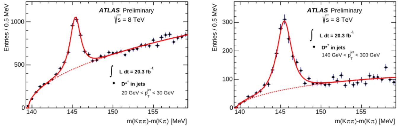
Figure 3 shows the distributions of the mass difference,∆m ≡m(Kππ)−m(Kπ), for theD^∗+candi- dates in the lowest and highest jet p_Tbins used in the analysis.

) [MeV]

π )-m(K π π m(K

140 145 150 155

Entries / 0.5 MeV

0 500 1000

ATLAS = 8 TeV s

Preliminary

< 30 GeV

jet T

20 GeV < p

-1

L dt = 20.3 fb

∫

in jets D*+

) [MeV]

π )-m(K π π m(K

140 145 150 155

Entries / 0.5 MeV

0 100 200 300

ATLAS = 8 TeV s

Preliminary

< 300 GeV

jet

140 GeV < pT -1

L dt = 20.3 fb

∫

in jets D*+

Figure 3: Mass difference distribution of theD^∗+candidates associated with jets with 20 GeV < pT <

30 GeV (left), and 140 GeV< p_T<300 GeV (right). The solid curve shows the fit to the distribution, as described in Sec. 4.3, while the dotted curve shows only the background contribution to the fit.

4.3 Method

A fit of the mass difference∆mdistribution in each jet pT interval being calibrated is done in order to determine the yield of theD^∗+mesons. The signal partS is fitted using a modified Gaussian function:

S ∝exp[−0.5·x^{(1+1+0.5x1 )}], x=|(∆m−∆m₀)/σ| (1)

which provides a better description of the signal tails than a simple Gaussian. The mean and width of the∆mpeak,∆m0andσ, are free parameters in the fit. The combinatorial backgroundBis fitted with a power function multiplied by an exponential function:

B∝(∆m−m_π)^αe^{−β(∆m−mπ)}, (2) whereαandβare also free fit parameters. The resulting fits in the lowest and highest jetp_Tbins are also shown in Figure 3.

Background subtraction technique

The selection ofD^∗+meson decays associated with jets allows background subtraction techniques to be used to perform comparisons between data and simulation in any variable related to theD^∗+mesons or jets, for the mixture ofbandcjets present in data.

Signal and background regions are defined as the region within 3σ of the∆mpeak centre and the region above 150 MeV, respectively. The choice of the∆mintervals for the (disjoint) signal and back- ground regions aims at including almost all the signal events in the signal region and ensuring a negligible fraction of signal events in the background region.

For each variable, the data distribution extraction proceeds as follows: the distribution of events from the background region, normalised to the fitted background fraction in the signal region, is subtracted from the corresponding distribution in the signal region.

The procedure relies on the assumption that the distribution of the variable of interest is the same for the combinatorial background under the peak and in the sideband. This assumption has been verified to be valid in simulated events. It is further supported by the observation in data that the distributions ob- tained from two different contiguous sideband regions (∆m∈[150,160] MeV and∆m∈[160,168] MeV) are compatible with each other within their statistical uncertainty.

Measuring the flavour composition in the background-subtracted D^∗+sample

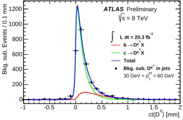
The measurement of the flavour composition for the selected D^∗+ sample is a key ingredient for its use inb-tagging calibration studies. The discriminating variable adopted to identify beauty and charm components is theD⁰pseudo-proper time defined as:

t(D⁰)=sign(L_xy(D⁰)·p_T(D⁰))·m_D0 ·L_xy(D⁰)

p_T(D⁰), (3)

where m_D0 is the D⁰ meson mass [20], p_T(D⁰) is the transverse momentum of the reconstructed D⁰ candidate, andLxy(D⁰) is the distance, in the transverse plane, between its decay vertex and the primary vertex in the event; pT(D⁰) andLxy(D⁰) are the vectorial equivalents of the latter two variables.

The fit used to extract the beauty fraction is described in Ref. [19]. Thet(D⁰) distribution for the charm component, Fc(t), is modelled as a single exponential function with a time constant equal to the measuredD⁰ lifetime [20], convolved with the pseudo-proper time resolution, described by the sum of a simple Gaussian and a modified Gaussian. The t(D⁰) distribution for the beauty component, F_b(t), is modelled as the convolution of two exponential functions, further convolved with the pseudo-proper time resolution. In this case, the choice of the model cannot be easily inferred from physics arguments, as the pseudo-proper time of D⁰candidates from beauty depends on many variables such as the beauty hadron and D⁰decay times, the momenta and the angle between their flight paths. Therefore the model that provides the best agreement with the simulated distribution is used.

Once the models for charm and beauty components are fixed, their sum is built asF(t)= f_b·F_b(t)+ (1−fb)·Fc(t), where fbis the fractional beauty abundance. A binned maximum likelihood fit is performed on background-subtracted data, using the variable ct(D⁰) in the range [-1, 2] mm, and leaving the fb

parameter free.

The fit to background-subtracted data, in the jet pT bin 30–60 GeV, is shown in Figure 4, and the results in the four bins of jet pT are summarised in Table 1 and used in the following section to evaluate thec-jet tagging efficiencies.

Measuring the c-jet tagging efficiency using D^∗+candidates

The selected sample is used to measure thec-jet tagging efficiency for jets associated withD^∗+ candi- dates, by performing a simultaneous fit to the∆mdistributions forD^∗+mesons in jets satisfying and not satisfying theb-tagging requirement.

The fit parameters describing the signal and the background shapes are required to be equal for the two distributions and the simultaneous fit only introduces theD^∗+tagging efficiencyϵD^∗+ as an extra

JetpT[GeV] Fitted fbvalue 20–30 0.193±0.017 30–60 0.197±0.014 60–140 0.157±0.014 140–300 0.171±0.023

Table 1: Beauty fractions determined by pseudo-proper time fits to the data in four jet p_T bins. Uncer- tainties are statistical only.

) [mm]

ct(D0

-1 -0.5 0 0.5 1 1.5 2

Bkg. sub. Events / 0.1 mm

0 200 400 600 800 1000

1200 ATLAS

= 8 TeV s

Preliminary

-1

L dt = 20.3 fb

∫

+

→ D*

c Total

in jets Bkg. sub. D*+

< 60 GeV

jet

30 GeV < pT

Figure 4: Fitted D⁰ pseudo-proper time distributions to background-subtractedD^∗+data samples in the jet p_Tbin 30–60 GeV. The solid lines show the complete fit (blue), the beauty component (red) and the charm component (green).

parameter accounting for the different yield ofD^∗+candidates in tagged and untagged jets. The procedure was tested in simulation and it has been verified that the measured efficiency on jets associated with a D^∗+meson is unbiased.

Using the method described it is possible to obtain the efficiency to tag jets associated with aD^∗+

candidate. This efficiency ϵD^∗+ is then decomposed into the efficiency forbandc jets containing D^∗+

using:

ϵD^∗+ = fbϵb(D^∗+)+(1− fb)ϵc(D^∗+), (4)

where fbis the fraction of D^∗+from beauty, before theb-tagging selection, determined by the fit to the pseudo-proper time distribution (see Table 1). The efficiency to tag a b jet, ϵb, is taken from simula- tion and corrected by the data-to-simulation scale factors obtained from theb-jet efficiency calibration analysis [2].

Extrapolation to inclusive charm

The calibration procedure described in the previous paragraph measures the c-jet tagging efficiency, and hence the corresponding scale factorκ^datac ^/sim(D^∗+) = ϵ_c^data(D^∗+)/ϵ^sim_c (D^∗+), forc → D^∗+(→ D⁰(→

K⁻π⁺)π⁺)X jets. Charm jets containing a D^∗+ meson are tagged more often than generic charm jets because of the requirement of having at least three reconstructed charged tracks. The extrapolation to a corresponding scale factorκ^datac ^/sim for inclusivecjets has to be evaluated.

The efficiency extrapolation factors,X, are defined by

ϵc^data = X^data·ϵc^data(D^∗+), (5)

ϵ_c^sim = X^sim·ϵ_c^sim(D^∗+), (6)

where ϵc(D^∗+) is the c-jet tagging efficiency measured in this analysis using jets associated with D^∗+

mesons andϵcis thec-jet tagging efficiency on a inclusive sample of cjets. The inclusivec-jet tagging scale factor is given by

κc^data/sim≡ ϵ_c^data ϵc^sim

= X^data

X^simκ^datac ^/sim(D^∗+). (7) The typical values ofX^sim, evaluated for the MV1 tagger, range between 0.5 and 0.7, depending on the working point. However, it is not currently possible to measure the corresponding factor in data.

The extrapolation factor in data can be different from that in simulation, either because the production fractions of the various charm hadron species are different, or because of different charged-particle mul- tiplicity distributions for the decays of a given charm hadron. The extrapolation factor in data is therefore estimated from simulation, after reweighting both the production fractions and branching ratios in the simulation to the best experimental values. In particular, for the production fractions a combination of the HERA and LEP measurements [21] is used, and for theD⁰branching ratios ton-prong final states, the values reported by the PDG [20]. No measurements are currently available for the branching ratio ton-prong final states for the other charm species, therefore the EvtGensimulation branching ratios are considered as central values.

The extrapolation factorX^data/X^simcan then be expressed as X^data

X^sim = ϵ^data/ϵ^data(D^∗+)

ϵ^sim/ϵ^sim(D^∗+) ≈ ϵcorr^sim/ϵcorr^sim(D^∗+) ϵ^sim/ϵ^sim(D^∗+) = ϵcorr^sim

ϵ^sim, (8)

since ϵ^sim(D^∗+) = ϵcorr^sim(D^∗+) (as the efficiency for the fully exclusive decay mode studied here is not affected by the correction reweighting procedure). In this equation, the second equality reflects the approximation of efficiencies in data by the ones in the simulation corrected for the above-mentioned effects.

The main discrepancies between the Monte Carlo simulation and the experimental knowledge are theΛ⁺c production fraction and the D⁰ → 0−prong decay branching ratio, which are both lower in the simulation. Since both of these lead to low tagging efficiencies (due to the short Λ⁺c lifetime and the absence of charged particles for theD⁰ →0−prong decays), the effect of the extrapolation procedure is to decrease the estimated inclusiveb-tagging efficiency. The extrapolation factor ranges indeed between 0.85 and 0.95, depending on the tagging working point. The variation with jet p_Tis a few percent only.

4.4 Systematic uncertainties

The dominant systematic uncertainties are those related to the fit of the yield of D^∗+ mesons, to the extractions of the fraction ofD^∗+mesons originating from beauty hadrons and to the extrapolation of the c-jet tagging efficiency scale factor measured on jets associated with aD^∗+meson to that of an inclusive c-jet sample. The sources of systematic uncertainty are discussed in more detail in the following and summarised in Table 2.

D^∗+mass fit and background parametrisation

The systematic uncertainty in the mass fit is evaluated by removing the constraint that the width of the D^∗+ mass peak and the parametrisation of the background shape are the same in the pre-tagged and tagged sample. The fit is repeated removing separately either of these constraints, and the resulting efficiency variations are taken as two separate systematic uncertainties.

b-tagging efficiency scale factor

The tagging efficiency for bjets is evaluated by multiplying the value found in simulation by the scale factor obtained in the b-jet performance calibration [2]. The variation of this scale factor within its uncertainty is propagated to the final result as a systematic uncertainty.

Beauty fraction fit

To study the effects of imperfect modelling of the pseudo-proper time resolution in simulation and the beauty lifetime uncertainty, the following procedure is adopted:

• Resolution systematics: the fit results have a weak dependence on the assumed resolution func- tions, and a conservative systematic uncertainty is assigned by fixing the Gaussian and modified Gaussian widths to 0.5 and 1.5 times the resolution fitted on the simulated sample. This mainly affects small pseudo-proper time values, while the fit results are mainly influenced by the beauty tails at high positive values.

• Lifetime uncertainty: the lifetimes of the two exponentials used in modelling the beauty compo- nent are each varied by the error obtained by fitting the template on simulated data (more details in Ref. [19]).

In both cases the maximum positive and negative variations in the beauty fraction central value are taken as an estimate of the corresponding systematic uncertainty. The total uncertainty on the beauty fraction is calculated by combining the fit statistical error together with the resolution and lifetime systematics, and is used to evaluate the systematic uncertainty on thec-jet tagging efficiency.

Jet energy scale

The systematic uncertainty originating from the jet energy scale is obtained by scaling thep_Tof each jet in the simulation up and down by one standard deviation, according to the uncertainty of the jet energy scale [11]. This systematic uncertainty impacts both the true c-jet tagging efficiency and the pseudo- proper time templates.

Jet energy resolution and jet vertex fraction

The jet energy resolution in data has been found to be generally well-modelled in simulation [22], and additional smearing was applied to the simulation in order to cover the uncertainties and residual differ- ences.

The jet vertex fraction requirement JVF>0.5 has been found to be very useful in removing pile-up jets from an event, but its distribution for pile-up jets is not very well modelled in the simulation [10]. A systematic uncertainty relating to JVF is calculated by varying the JVF cut values in simulated events to cover the observed discrepancies with the data.

Extrapolation

The uncertainties on the extrapolation factor are obtained by varying individually each charm production fraction andD⁰→n−prong branching ratio within its experimental uncertainty. For then−prong branch- ing ratios of the other charm species no experimental measurements are available; therefore the largest difference between the EvtGen(default used in the simulation) and either Pythiaor Herwigsimulations is used to evaluate the systematic uncertainties. A further systematic uncertainty due to possible mis- modelling of thec-quark fragmentation functions is evaluated by taking the difference between Pythia and Herwigsimulations.

4.5 Results

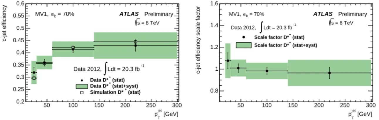
The measuredc-jet tagging efficiencies in data, thec-jet tagging efficiencies in simulation and the result- ing data-to-simulation scale factors for the 70% efficiency working point of the MV1 tagging algorithm are shown in Fig. 5, for jets containing D^∗+ mesons. The corresponding results after extrapolation to inclusive charm jets are shown in Fig. 6. The systematic and statistical uncertainties on thec-jet tagging efficiency scale factors for the 70% efficiency MV1 working point are shown in Table 2. The total un- certainties for this working point range between 8% and 15%. The scale factors are around 0.9, caused mostly by the extrapolation to inclusive charm jets. No significant p_Tdependence is observed. Similar conclusions hold for other working points.

[GeV]

jet

pT

50 100 150 200 250 300

c-jet efficiency

0.2 0.25 0.3 0.35 0.4 0.45 0.5 0.55 0.6

Data 2012,

∫

(stat+syst) Data D*+

(stat) Simulation D*+

ATLAS Preliminary = 8 TeV s

∈ MV1, _b = 70%

[GeV]

jet

pT

50 100 150 200 250 300

c-jet efficiency scale factor

0.8 1 1.2 1.4 1.6

(stat) Scale factor D*+

(stat+syst) Scale factor D*+

ATLAS Preliminary = 8 TeV s

∈ MV1, b = 70%

Data 2012,

∫

Figure 5: Thec-jet tagging efficiency in data and simulation (left) and the data-to-simulation scale factor (right) for jets containingD^∗+, for the 70% working point of the MV1 tagger.

[GeV]

jet

pT

50 100 150 200 250 300

c-jet efficiency scale factor

0.6 0.8 1 1.2 1.4

Scale factor inclusive (stat) Scale factor inclusive (stat+syst)

ATLAS Preliminary = 8 TeV s

∈ MV1, b = 70%

Data 2012,

∫

Figure 6: Data-to-simulation scale factor for inclusive charm jets, after the extrapolation procedure de- scribed in Sec. 4.3, for the 70% working point of the MV1 tagger.

5 Mistag rate calibration

The mistag rate is defined as the fraction of jets originating from light flavour which are tagged by a b-tagging algorithm. The mistag rate is measured in an inclusive jet sample, using the negative tag method.

Source Jetp_T[GeV]

20–30 30–60 60–140 140–300

Scale factor 0.97 0.90 0.86 0.86

D^∗+mass fit 9.4 2.8 3.4 5.1

background parametrisation 2.5 1.1 0.7 0.5

b-jet efficiency scale factor 4.5 1.2 0.7 2.0

beauty fraction fit 4.5 3.5 2.7 8.5

jet energy scale 4.4 1.3 0.5 1.9

jet energy resolution 0.7 0.1 0.4 1.4

jet vertex fraction 0.7 0.1 <0.1 <0.1

extrapolationc→D⁺ 1.2 1.1 0.8 0.7

extrapolationc→D⁰ 0.7 0.6 0.4 0.5

extrapolationc→Ds <0.1 <0.1 0.1 0.1

extrapolationc→Λc 2.1 2.0 1.9 1.5

extrapolationD⁰ →4 prongs 0.2 0.2 0.2 0.2 extrapolationD⁰ →2 prongs 0.2 0.5 1.0 0.5 extrapolationD⁰ →0 prongs 2.2 3.2 4.6 3.9

extrapolationD⁺→prongs 0.9 0.9 0.8 0.7

extrapolationD_s→prongs 1.0 1.1 1.3 1.2

extrapolationΛc →prongs 0.2 0.2 0.2 0.1

extrapolation fragmentation 1.9 1.3 0.8 0.6

systematic uncertainty 13 6.6 7.0 11

statistical uncertainty 6.8 3.9 3.1 5.4

total uncertainty 15 7.7 7.7 13

Table 2: Data-to-simulationc-jet tagging efficiency scale factors for the MV1 tagging algorithm at 70%

efficiency; and corresponding relative systematic and statistical uncertainties, in %.

5.1 Data and simulation samples

The event sample for the mistag rate measurement was collected using a logical OR of single jet triggers, analogous to that used in the D^∗ analysis (see Sec. 4). At least two jets are required in each event, and the two leading jets must be separated in azimuth by∆ϕ > 2. The mistag rate is then measured on the sample obtained by using only the leading jet in each event.

The analyses also make use of simulated multijet samples, similar to those used in the D^∗ c-jet tagging efficiency measurement, but without anyD^∗filter.

5.2 The negative tag method

Light-flavour jets are tagged asbjets mainly because of the finite resolution of the inner detector and the presence of tracks from displaced vertices of long-lived particles or material interactions. For prompt tracks the distributions of the lifetime-signed impact parameter (the sign is chosen positive if the angle between the jet direction and the line joining the primary vertex to the point of closest approach is less than π/2, and negative otherwise) and of the signed decay length of vertices reconstructed using these tracks are expected to be symmetric.

The inclusive tag rate obtained by reversing the impact parameter significance sign of tracks for impact parameter based tagging algorithms, or reversing the decay length significance sign of secondary vertices for secondary vertex based tagging algorithms, is therefore expected to be a good approximation of the mistag rate due to resolution effects. For the MV1 tagging algorithm, the negative tag rate is computed by defining a negative version of the tagging algorithm which internally reverses the impact parameter and the decay length selections. A jet is then considered negatively tagged if the tag weight discriminant variable computed by this negative tagger version satisfies the normal weight criterion.

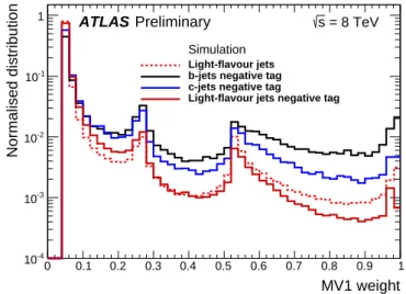
Figure 7 shows the standard and negative weight distributions for the MV1 algorithm in simulation.

While the tag weight distributions for b andc jets differ greatly between the two choices of tagging, the standard and negative tag weight distributions for light-flavour jets are substantially more similar in shape.

MV1 weight

0 0.1 0.2 0.3 0.4 0.5 0.6 0.7 0.8 0.9 1

Normalised distribution

10-4

10-3

10-2

10-1

1 ATLAS Preliminary s = 8 TeV

Simulation Light-flavour jets b-jets negative tag c-jets negative tag

Light-flavour jets negative tag

Figure 7: The MV1 negative tag weight distributions forb,cand light-flavour jets, as well as the standard MV1 weight distribution for light-flavour jets (dashed line), in simulation.

The mistag rateϵlis then estimated as the negative tag rate of the inclusive jet sample,ϵ_inc^neg, corrected for two further effects:

• As can be seen from Fig. 7, the negative tag rate forbandcjets differs from that for light-flavour jets. The bandcjets are tagged mainly because of the measurable lifetimes ofb- andc-hadron decays, shifting impact parameter and decay length significance distributions towards larger val- ues. However, effects like the finite jet direction resolution can flip the sign of the discriminating variable, increasing significantly the negative tag rate forbandcjets. A correction factork_hf=ϵ_l^neg /ϵ_inc^negis defined to account for this effect. Because of the effects described above and the relatively small fractions ofb andcjets in the inclusive sample, khf is typically smaller than, but close to unity.

• A symmetric decay length or impact parameter significance distribution for light-flavour jets is only expected for fake secondary vertices arising e.g. from track reconstruction resolution effects.

However, a significant fraction of reconstructed secondary vertices have their origin in charged particle tracks stemming from long-lived particles (KS,Λetc.) or material interactions (hadronic interactions and photon conversions). These vertices will show up mainly at positive decay length significances and thus cause an asymmetry for the positive versus negative tag rate for light-flavour jets. A correction factorkll=ϵl /ϵ_l^negis defined to account for this effect. Because of the sources in light-flavour jets showing positive decay length,k_llis larger than unity. For the MV1 algorithm in particular,k_llranges between 1 and 13, depending on the jetp_T and on the operating point. For the 70% working point, it ranges between 1 and 3.

The measured negative tag rate value ϵ_inc^neg is converted to mistag rate ϵl using the two correction factorsk_hfandk_lldefined above: ϵl =ϵ_inc^negk_hfk_ll. Both correction factors are inferred from the simulated samples.

5.3 Systematic uncertainties

The main systematic uncertainties affecting the mistag rate calibration are discussed in the following, and summarised in Tables 3 and 4 for jets with |η| < 1.2 and 1.2 < |η| < 2.5, respectively. In cases where the statistics in simulation are not sufficient to evaluate the effect of a given systematic variation, the systematic uncertainty has been evaluated by merging two adjacent jet pTbins.

Simulation statistics

The statistical uncertainties on k_hf and k_ll have been propagated through the analysis. The resulting uncertainties range between 1% and 7%.

Jet energy scale

A bias in the jet energy measurement in simulation compared to data will result in biases in the correction factorskhf andkllif there is a correlation between the jet energy and these quantities. As the mistag rate increases with the jet energy, a shift in the jet energy scale in simulated events will also lead to an apparent mismatch between the mistag rate in data and simulated events. The resulting uncertainties are below 4%.

Jet energy resolution

The uncertainty on the jet energy resolution is estimated by an additional smearing of the jet energies in simulated events [22]. The difference from the nominal mistag rate is 12% for the first bin in the forward region and below 6% for all other bins.

Sample dependence

Generally, only one of the two leading jets is in the jet p_T region where the single-jet trigger used to select the events is fully efficient. Therefore, any mismodelling in the simulation of the trigger turn-on behaviour can lead to a bias. For example, it is found that the number of tracks associated to the leading and sub-leading jets in a given jetp_Tinterval differs in data but not to the same extent in simulated events.

In order to account for possible trigger effects, the measurement has been repeated using only jets with sub-leadingpT. The variation in the mistag rate is taken as a systematic uncertainty.

Data taking period dependence

The analysis shows a dependence of the scale factor on the data taking periods of up to 14%, evaluated by taking the root mean square of the mistag rate scale factors from different data taking periods. This effect may be related to biases introduced by the trigger selection (the inclusive jet triggers used in these analyses have undergone substantial changes in the prescale factors applied to them with evolving in- stantaneous luminosity) which have not been modelled in the selection of simulated events. Run periods with different instantaneous luminosity show also a dependence of the mistag rate due to the different amount of pile-up vertices.

Heavy flavour fractions

The fractions ofb andc jets enter directly into the correction factor khf for the negative tag analysis.

Uncertainties on theb- andc-jet fractions of 10% and 30% have been propagated through the analysis, resulting in uncertainties which are generally below 5%. These uncertainties are estimated by fitting templates of distributions that discriminate between the different flavours, e.g. the invariant mass of tracks significantly displaced from the primary vertex, to the data.

Heavy flavour tagging efficiencies

The tagging efficiencies forbandcjets directly enter into the negative tag analysis through the correction factork_hf. Theb- andc-jet efficiencies as obtained from simulation have been varied by 20% and 40%, respectively. The variations used for theb- andc-jet efficiencies have conservatively been doubled com- pared to the uncertainties derived using the corresponding b-jet performance calibration [2] and those quoted in Section 4, to account for the extrapolation from the positive tagging efficiency to the negative one. The resulting uncertainties are generally below 6% (9%) forbjets (cjets).

Long-lived particle decays, material interactions, fake tracks and photon conversions

The products of the decays of long-lived particles, e.g. K_S,Λ, hadronic interactions or photon conver- sions in the detector material (mainly interactions in the first material layers of the detector), may cause reconstructed secondary vertices in light-flavour jets. While the secondary vertex based algorithms apply a veto to secondary vertices consistent with these decays or interactions, not all of them can be detected and there is a sizeable fraction of vertices where one track arising from such decays or interactions is paired with a track from a different source to create a vertex. Fake or badly measured tracks and photon conversions may also give rise to additional vertices.

To estimate the resulting systematic uncertainty from an imperfect modelling of the rate of such vertices in simulated events, the fraction of jets containing fake tracks, long-lived particles, material interactions or photon conversions have been varied based on estimates in data. The modelling of fake tracks is evaluated by fitting the track parameter χ²/DOF distribution in data to a weighted sum of templates for true and fake tracks obtained in MC. The MC tracks are categorised as fake if the fraction

of hits due to other particles is more than 80%. This fraction is determined using the hit MC truth information. The fraction of jets withK_S orΛdecays in data and simulation are compared by counting the number of events in the K_S andΛmass peaks. Finally, a jet with a hadronic interaction or photon conversion is estimated in simulated events as a jet containing a selected track which originates from a vertex separated from the beam line by at least 25 mm. It is found that about 80% of all jets have at least one such track. The uncertainty on the interaction rate in the material is evaluated by fitting the data 1/|ηi−ηj|distribution (whereηis the track pseudorapidity) for all track pairs in a jet to a weighted sum of MC templates for tracks from conversion pairs and any other track pairs, and comparing the results of the fit to the MC prediction. As the opening angle between the tracks from conversion pairs is small, they contribute to the tail of the distribution. In all cases, the difference between the data and the MC prediction is evaluated separately for each jet p_Tandηbin and converted to the corresponding uncertainty in the mistag rate scale factor.

Track multiplicity

The simulation does not properly reproduce the multiplicity of tracks associated with jets observed in data. This could be due to imperfect modelling of fragmentation differences in the relative fraction of quark and gluon jets in the light-flavour sample or differences in the track reconstruction efficiency between data and simulation. A higher track multiplicity implies a larger probability of accidentally tagging a light-flavour jet as abjet for purely combinatorial reasons. The systematic uncertainty in the negative tag analysis due to the track multiplicity is estimated by reweighting the jet sample according to the ratio of distributions of the number of tracks associated to jets in data and simulation in each kinematic bin. The effect of the track multiplicity reweighting ranges between approximately 4% at medium jetp_T and about 40% at lowest jet pT bin in the forward region. The track multiplicity systematic uncertainty affects the lowest jet pT bin most because the discrepancy between data and simulation is larger in that region.

Impact parameter smearing

Inclusive secondary vertex reconstruction is very sensitive to the tracking resolution and the proper es- timation of the track parameter errors. The track impact parameter resolutions in simulation are slightly better than those in data; therefore, track impact parameters in the simulation have been smeared in order to bring data and simulation into agreement. The chosen smearing approach does not take into account correlated modifications of the impact parameters of tracks that pass through the same pixel module, as would be needed to model residual misalignments in the inner detector. The parameters for the smearing have been chosen to cover the observed differences in the impact parameter resolution between data and simulation. After having applied the track impact parameter smearing to the tracks in simulation, the primary vertex reconstruction andb-tagging have been rerun and the whole analyses repeated. The effect in the negative tag analysis is approximately 5% in the centralηregion but can be as large as 22% in the forwardηregion where the modelling of the impact parameter resolution is worse.

5.4 Results

The measured mistag rates in data and in simulation, along with the resulting data-to-simulation scale factors for the MV1 tagging algorithm at 70% efficiency are shown in Figure 8. For the chosen working point the mistag rate ranges between 0.5% to 2.5%. The data/MC mistag rate scale factors are slightly larger than unity, with relative total uncertainties ranging between 15% and 43%.

Source Jet pT[GeV]

20–30 30–60 60–140 140–300 300–450 450–750

Scale factor 1.20 1.32 1.22 1.39 1.47 1.25

simulation statistics 5.6 2.7 1.5 1.8 1.8 1.6

jet energy scale 1.4 3.9 0.2 1.0 0.5 0.6

jet energy resolution 0.7 0.3 2.2 1.4 0.6 2.9

sample dependence 4.7 4.7 2.9 6.5 1.0 0.4

data taking period dependence 4.4 2.1 1.0 0.6 0.5 0.4

k_hf:bfraction 0.9 0.5 1.7 2.7 2.9 2.5

khf:cfraction 0.7 2.2 4.4 5.7 5.5 5.1

k_hf:b-jet efficiency 2.5 1.4 4.0 5.8 6.2 6.2

k_hf:c-jet efficiency 2.9 4.9 8.0 9.3 9.0 9.3

kll: long lived particles 0.2 0.2 0.4 1.1 1.0 0.6

kll: hadronic interactions 0.3 1.2 1.8 5.8 4.2 1.7

k_ll: fake tracks <0.1 0.9 0.6 2.8 2.5 1.1

kll: photon conversions 0.1 0.6 0.6 1.7 1.6 1.0

track multiplicity 29 11 11 5.3 3.8 6.1

impact parameter smearing 2.9 2.9 5.8 5.8 3.6 3.6

systematic uncertainty 30 15 17 18 15 15

statistical uncertainty 4.4 2.1 1.0 0.6 0.5 0.4

total uncertainty 31 15 17 18 15 15

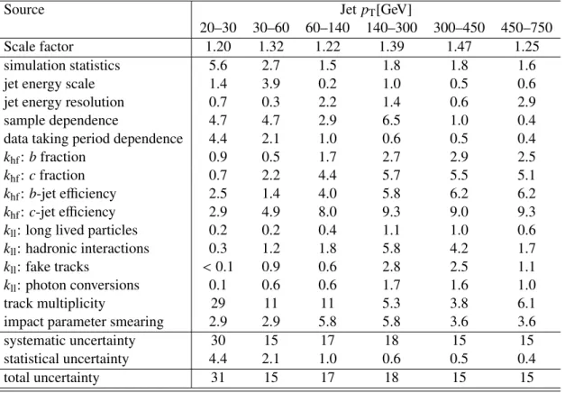
Table 3: Mistag rate scale factor κ_l^data/sim from the negative tag method for the 70% efficiency MV1 tagging working point for jets with|η|<1.2; and corresponding relative systematic and statistical uncer- tainties, in %.

Source Jet pT[GeV]

20–30 30–60 60–140 140–300 300–450 450–750

Scale factor 1.12 1.35 1.33 1.48 1.53 1.40

simulation statistics 7.0 3.2 1.8 1.8 2.6 4.9

jet energy scale 2.0 2.1 0.5 1.0 1.1 1.7

jet energy resolution 11 1.7 0.6 2.9 0.6 5.6

sample dependence 4.6 4.6 4.4 3.0 1.6 5.9

data taking period dependence 6.0 2.8 1.5 1.1 1.2 0.9

k_hf:bfraction 0.1 0.2 0.9 1.4 1.5 1.4

khf:cfraction 0.6 1.4 2.7 3.1 3.0 2.2

k_hf:b-jet efficiency 0.7 0.9 2.5 3.2 3.3 3.4

k_hf:c-jet efficiency 2.8 3.8 5.7 6.0 5.8 5.0

kll: long lived particles 0.4 0.1 0.3 0.8 0.2 0.5

kll: hadronic interactions 0.1 1.9 2.7 7.9 6.7 2.9

k_ll: fake tracks 0.4 0.4 0.1 0.7 2.0 0.5

kll: photon conversions <0.1 1.3 1.2 3.6 3.0 0.5

track multiplicity 38 14 16 8.3 4.9 8.9

impact parameter smearing 11 11 10 10 22 22

systematic uncertainty 42 20 21 18 25 27

statistical uncertainty 5.9 2.7 1.5 1.1 1.1 0.9

total uncertainty 43 20 21 18 25 27

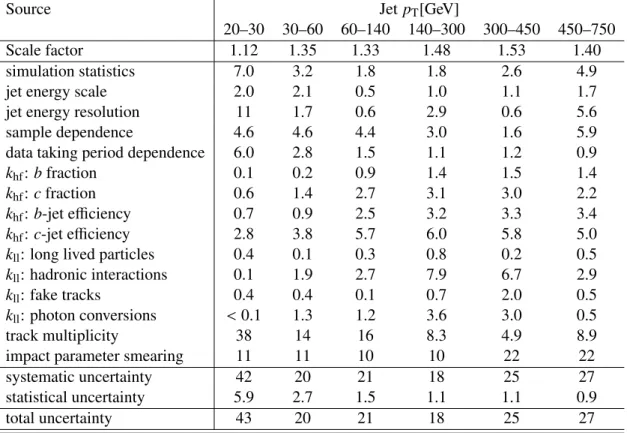
Table 4: Mistag rate scale factor κ_l^data/sim from the negative tag method for the 70% efficiency MV1 tagging working point for jets with 1.2< |η|< 2.5; and corresponding relative systematic and statistical uncertainties, in %.

[GeV]

jet

pT

30 40 50 100 200 300

Mistag rate

0 0.005 0.01 0.015 0.02 0.025 0.03 0.035 0.04

Data (stat) Data (stat+syst) Simulation (stat)

ATLAS Preliminary

∫

∈b

MV1, |η^jet| < 1.2

[GeV]

jet

pT

30 40 50 100 200 300

Mistag rate

0 0.005 0.01 0.015 0.02 0.025 0.03 0.035 0.04

Data (stat) Data (stat+syst) Simulation (stat)

ATLAS Preliminary

∫

∈b

MV1, 1.2 < |η^jet| < 2.5

[GeV]

jet

pT

30 40 50 100 200 300

Mistag rate scale factor

0.8 1 1.2 1.4 1.6 1.8 2 2.2 2.4

Scale factor (stat) Scale factor (stat+syst)

ATLAS Preliminary

∫

∈b

MV1, |η^jet| < 1.2

[GeV]

jet

pT

30 40 50 100 200 300

Mistag rate scale factor

0.6 0.8 1 1.2 1.4 1.6 1.8 2 2.2 2.4

Scale factor (stat) Scale factor (stat+syst)

ATLAS Preliminary

∫

∈b

MV1, 1.2 < |η^jet| < 2.5

Figure 8: The mistag rate in data and simulation (top) and the data-to-simulation scale factor (bottom) for the MV1 tagging algorithm at 70% efficiency obtained with the negative tag method, for jets with

|η|<1.2 (left) and jets with 1.2<|η|<2.5 (right).

6 Conclusions

The b-tagging efficiency ofcand light-flavour jets for severalb-tagging algorithms has been measured with 20.3 fb⁻¹ of data collected by the ATLAS detector in ppcollisions at 8 TeV. The results are ex- pressed in terms of scale factors, correcting the efficiencies in simulated events to those measured in data. The reference multivariate tagger (MV1) at 70% efficiency has been used as a benchmark.

ReconstructedD^∗+ mesons associated with jets have been exploited to measure theb-tagging effi- ciency oncjets. The scale factors are consistent with unity with uncertainties varying, depending on the jet p_T, from 8% to 15%.

The negative-tag method has been used to measure the light-jet efficiency (mistag rate) scale factors.

They are found to be larger than unity with a precision ranging between 15% and 43% depending on the p_Tandηregions.

References

[1] ATLAS Collaboration,The ATLAS Experiment at the CERN Large Hadron Collider, JINST3 (2008) S08003.

[2] ATLAS Collaboration,Calibration of b-tagging using dileptonic top pair events in a combinatorial likelihood approach with the ATLAS experiment, ATLAS-CONF-2014-004, http://cdsweb.cern.ch/record/1664335.

[3] ATLAS Collaboration,Performance of the ATLAS Secondary Vertex b-tagging Algorithm in 7 TeV Collision Data, ATLAS-CONF-2010-042,http://cdsweb.cern.ch/record/1277682.

[4] ATLAS Collaboration,Commissioning of high performance b-tagging algorithms with the ATLAS detector, ATLAS-CONF-2011-102,http://cdsweb.cern.ch/record/1369219.

[5] W. Lampl et al.,Calorimeter Clustering Algorithms: Description and Performance, ATL-LARG-PUB-2008-002. ATL-COM-LARG-2008-003.

[6] M. Cacciari, G. P. Salam, and G. Soyez,The anti-k_t jet clustering algorithm, JHEP04(2008) 063, arXiv:0802.1189 [hep-ph].

[7] M. Cacciari and G. P. Salam,Dispelling the N³myth for the k_t jet-finder, Phys. Lett.B641(2006) 057,arXiv:0512210 [hep-ph].

[8] M. Cacciari, G. P. Salam, and G. Soyez. http://fastjet.fr/.

[9] M. Cacciari and G. P. Salam,Pileup subtraction using jet areas, Phys. Lett.B659(2008) 119–126, arXiv:0707.1378 [hep-ph].

[10] ATLAS Collaboration,Pile-up subtraction and suppression for jets in ATLAS, ATLAS-CONF-2013-083,http://cds.cern.ch/record/1570994.

[11] ATLAS Collaboration,Jet energy measurement with the ATLAS detector in proton- proton collisions at √

s=7TeV, Eur. Phys. J.C73(2013) 2304,arXiv:1112.6426 [hep-ex].

[12] T. Sj¨ostrand, S. Mrenna, and P. Z. Skands,A Brief Introduction to PYTHIA 8.1, Comput. Phys.

Commun.178(2008) 852–867,arXiv:0710.3820 [hep-ph].

[13] GEANT4 Collaboration, S. Agostinelli et al.,GEANT4: A simulation toolkit, Nucl. Instrum. Meth.

A506(2003) 250–303.

[14] ATLAS Collaboration,The ATLAS Simulation Infrastructure, Eur. Phys. J.C70(2010) 823–874, arXiv:1005.4568 [physics.ins-det].

[15] T. Sj¨ostrand, S. Mrenna, and P. Z. Skands,PYTHIA 6.4 Physics and Manual, JHEP05(2006) 026.

[16] P. Z. Skands,Tuning Monte Carlo Generators: The Perugia Tunes, Phys. Rev.D82(2010) 074018,arXiv:1005.3457 [hep-ph].

[17] H. L. Lai et al.,New parton distributions for collider physics, Phys. Rev.D82(2010) 074024, arXiv:1007.2241 [hep-ph].

[18] D. J. Lange,The EvtGen particle decay simulation package, Nucl. Instr. Meth.A462(2001) 152.

[19] ATLAS Collaboration,b-jet tagging calibration on c-jets containing D^⋆mesons, ATLAS-CONF-2012-039,http://cdsweb.cern.ch/record/1435193.

[20] J. Beringer et al.,Review of Particle Physics (RPP), Phys. Rev.D86(2012) 010001, and 2013 partial update for the 2014 edition.

[21] E. Lohrmann,A Summary of Charm Hadron Production Fractions,arXiv:1112.3757v1 [hep-ex].

[22] ATLAS Collaboration,Jet energy resolution and reconstruction efficiencies from in-situ

techniques with the ATLAS Detector Using Proton-Proton Collisions at a Center of Mass Energy

√s=7TeV, ATLAS-CONF-2010-054,http://cdsweb.cern.ch/record/1281311.