e.g. the fluctuations of the topological charge are related to the mass of the flavour-singlet pseudoscalar

https://doi.org/10.1140/epjc/s10052-020-7984-9

Regular Article - Theoretical Physics

Comparison of topological charge definitions in Lattice QCD

Constantia Alexandrou^1,2, Andreas Athenodorou^1,2,a, Krzysztof Cichy^3,b , Arthur Dromard⁴, Elena Garcia-Ramos^5,6, Karl Jansen⁵, Urs Wenger⁷, Falk Zimmermann⁸

1Department of Physics, University of Cyprus, P.O. Box 20537, 1678 Nicosia, Cyprus

2Computation-based Science and Technology Research Research, The Cyprus Institute, 20 Kavafi Str., Nicosia 2121, Cyprus

3Faculty of Physics, Adam Mickiewicz University, ul. Uniwersytetu Poznanskiego 2, 61-614 Pozna´n, Poland

4Institute for Theoretical Physics, Regensburg University, 93053 Regensburg, Germany

5NIC, DESY, Platanenallee 6, 15738 Zeuthen, Germany

6Humboldt Universität zu Berlin, Newtonstr. 15, 12489 Berlin, Germany

7Universität Bern, Albert Einstein Center for Fundamental Physics, Institute for Theoretical Physics, Sidlerstrasse 5, 3012 Bern, Switzerland

8Helmholtz-Institut für Strahlen- und Kernphysik (Theorie) and Bethe Center for Theoretical Physics, Universität Bonn, 53115 Bonn, Germany

Received: 16 December 2019 / Accepted: 28 April 2020

© The Author(s) 2020

Abstract

In this paper, we show a comparison of different definitions of the topological charge on the lattice. We con- centrate on one small-volume ensemble with 2 flavours of dynamical, maximally twisted mass fermions and use three more ensembles to analyze the approach to the continuum limit. We investigate several fermionic and gluonic defini- tions. The former include the index of the overlap Dirac operator, the spectral flow of the Wilson–Dirac operator and the spectral projectors. For the latter, we take into account different discretizations of the topological charge operator and various smoothing schemes to filter out ultraviolet fluc- tuations: the gradient flow, stout smearing, APE smearing, HYP smearing and cooling. We show that it is possible to perturbatively match different smoothing schemes and pro- vide a well-defined smoothing scale. We relate the smoothing parameters for cooling, stout and APE smearing to the gra- dient flow time

. In the case of hypercubic smearing the matching is performed numerically. We investigate which conditions have to be met to obtain a valid definition of the topological charge and susceptibility and we argue that all valid definitions are highly correlated and allow good con- trol over topology on the lattice.

1 Introduction

QCD gauge fields can have non-trivial topological proper- ties, manifested in non-zero and integer values of the so- called topological charge. Such topological properties are believed to have important phenomenological implications,

ae-mail:andreas.athinodorou@pi.infn.it

be-mail:kcichy@amu.edu.pl(corresponding author)

e.g. the fluctuations of the topological charge are related to the mass of the flavour-singlet pseudoscalar

meson [1,2].

The topology of QCD gauge fields is a fully non-perturbative issue, hence lattice methods are well-suited to investigate it.

Naively, lattice gauge fields are topologically trivial, since they can always be continuously deformed to the unit gauge field. However, it can be shown that for smooth enough gauge fields (sufficiently close to the continuum limit), the notion of topology of lattice gauge fields is still meaningful [3]. Histor- ically, the first investigation aimed at studying the topologi- cal properties of a non-Abelian gauge theory was reported in Refs. [4,5] for the SU(2) gauge group case and then extended to SU(3) in Ref. [6].

Over the years, many definitions of the topological charge

of a lattice gauge field were proposed [7,8]. It is clear that

the definitions differ in terms of their computational cost and

convenience, but also theoretical appeal. These definitions

can be characterized either as fermionic or gluonic. During

the last decade, a number of efforts have revealed impor-

tant aspects of the topological susceptibility, which reflects

the fluctuations of the topological charge. Universality of the

topological susceptibility in fermionic definitions has been

demonstrated [9], giving an insight in the basic properties a

definition has to obey so that the topological susceptibility

is free of short-distance singularities, which have plagued

some of the earlier attempts at a proper and computation-

ally affordable fermionic definition [10,11]. On the other

hand, considering the gluonic definition, a theoretically clean

understanding on how the topological sectors emerge in the

continuum limit has been attained through the gradient flow

[12–16]. Further projects have also divulged the numerical

equivalence of the gradient flow with the smoothing tech-

nique of cooling at finite lattice spacing. Previous investi- gations, on the other hand, have shown numerically that the field theoretic topological susceptibility extracted with sev- eral smoothing techniques such as cooling, APE and HYP smearing give the same continuum limit. Although no solid theoretical argument suggests so, it is believed that all differ- ent definitions of the topological charge agree in the contin- uum limit. Good agreement has also been found between the gluonic definiton and a fermionic one in finite-temperature studies [17]. For an overview of topology-related issues on the lattice, we refer to the review paper by Müller-Preussker [8].

This aim of the paper is two-fold. The first purpose is to investigate the perturbative equivalence between the smooth- ing schemes of the gradient flow, cooling as well as APE, stout and HYP smearing. In Refs. [18,19] it was demon- strated that gradient flow and cooling are equivalent if the gradient flow time

and the number of cooling steps n

are appropriately matched. By expanding the gauge links pertur- batively in the lattice spacing a, at subleading order, the two methods become equivalent if one sets

n

15b

where b

is the Symanzik coefficient multiplying the rect- angular term of the smoothing action. It is, thus, interesting to extend the study of Ref. [18] and explore whether similar matching can also be derived for APE, stout and HYP smear- ings. Hence, we carry out such investigation and support it with the appropriate numerical results.

The second motivation of this paper is to attempt a system- atic investigation of different topological charge definitions.

We have computed them on selected ensembles generated by the European Twisted Mass Collaboration (ETMC)

. The included definitions are:

– index of the overlap Dirac operator on HYP-smeared and non-HYP-smeared configurations,

– Wilson-Dirac operator spectral flow (SF), – spectral projector definition,

– field theoretic (gluonic) definition, with gauge fields smoothed using:

– gradient flow (GF) with different smoothing actions and at different flow times. Namely, we smooth the gauge fields using the Wilson plaquette, Symanzik tree-level and Iwasaki actions at flow times t

, 2t

and 3t

; t

is defined in Sect.

– cooling (cool) with the three different smoothing actions and cooling steps matched to GF time for t

, 2t

and 3t

,

1In 2019, the name of the collaboration has been changed to Extended Twisted Mass Collaboration.

2For references on each of the following definitions, we refer to Sect.3.4.

– stout smearing with three different values of the stout parameter

and smearing steps matched to GF time at flow times t

, 2t

and 3t

,

– APE smearing with three different values of the parameter

and smearing steps matched to GF time for t

, 2t

and 3t

,

– HYP smearing for a given set of parameters

,

,

, and smearing steps numerically matched to GF time at flow times t

, 2t

and 3t

.

The outline of the paper is as follows: Sect.

describes our lattice setup as well as the relevant details regarding the production of the N

2 configurations. Section

intro- duces the topological charge definitions that we are using and includes the derivation of matching conditions between different smoothing schemes. In Sect.

pare different definitions of the topological charge, we ana- lyze the approach to the continuum limit and we show results for the topological susceptibility. Finally, in Sect.

we sum- marize and conclude.

2 Lattice setup

Motivated by the desire to cover as many definitions of the topological charge as possible, including the costly overlap definition, we performed our comparison of different topo- logical charge definitions on small volume ensembles (to keep the computational cost affordable and at the same time incorporate all definitions) generated by ETMC with N

2 [20–22] dynamical twisted mass fermions. The action in the gauge sector is

S

3

x

b

4

μ,ν=1 1≤μ<ν

Re Tr

1

P

+

b

4

μ,ν=1 μ=ν

Re Tr

1

P

,

(1)

with

6/g

, g

being the bare coupling and P

, P

the plaquette and rectangular Wilson loops respectively. The configurations were generated with the tree-level Symanzik improved action [23], i.e. b

, b

1

8b

. Note that for smoothing the gauge fields using the gradient flow and cooling, in addition to the tree-level Symanzik improved action, we use the Wilson plaquette action which corresponds to b

0 and b

1 as well as the Iwasaki improved action with b

b

3.648.

The fermionic action for the light quarks is the Wilson

twisted mass action [24–27], given in the so-called twisted

Table 1 Parameters of the employed ETMCN_f =2 gauge field con- figuration ensembles [20–22]. The columns contain: the inverse bare couplingβ, the approximate values of the lattice spacinga[28–30], r₀/a[28,30], the scheme- and scale-independent renormalization con-

stants ratioZ_P/Z_S[31–33], the lattice size(L/a)³×(T/a), the bare twisted light quark massaμl, the critical value of the hopping parameter (where the PCAC mass vanishes), physical extentLof the lattice in fm and the productm_πL

Ensemble β a[fm] r₀/a Z_P/Z_S lattice aμl κc L[fm] m_πL

b40.16 3.90 0.085 5.35(4) 0.639(3) 16³×32 0.004 0.160856 1.4 2.5

c30.20 4.05 0.067 6.71(4) 0.682(2) 20³×40 0.003 0.157010 1.3 2.4

d20.24 4.20 0.054 8.36(6) 0.713(3) 24³×48 0.002 0.154073 1.3 2.4

e17.32 4.35 0.046 9.81(13) 0.740(3) 32³×64 0.00175 0.151740 1.5 2.4

basis by

S

U] = a

x

¯ χl(x)

D

χl(x) ,

(2)

where

acts in flavour space and

is a two-component vector in flavour space, related to the one in the physical basis (

) by a chiral rotation,

exp(i

, with

being the twist angle (ω

maximal twist). The bare untwisted and twisted quark masses are, respectively, m

and

, while the multiplicatively renor- malized light quark mass is

Z

. D

is given by:

D

1 2

γμ(∇μ+ ∇_μ^∗)−

a

,

(3)

where

and

represent the forward and backward covari- ant derivatives, respectively.

Twisted mass fermions are providing an automatically

twist). This can be achieved by non-perturbative tuning of the hopping parameter

8

2am

to its critical value, i.e. such that the PCAC quark mass vanishes [25,34–38].

The details of the gauge field configuration ensembles that were used in this work are shown in Table

of our investigations are performed using the ensemble b40.16. However, we also investigate how the correlation between different topological charge definitions changes when approaching the continuum limit, thus using also ensembles c30.20, d20.24 and e17.32. For all of these ensem- bles the pion mass is close to 340 MeV

3 Definitions of the topological charge

In this section, we introduce the definitions of the topological charge that we use below for numerical studies. We attempted to include the most commonly used, theoretically sound defi- nitions of the topological charge. The relevant characteristics of each definition are summarized in Table

3.1 Index of the overlap Dirac operator

For many years, it was considered impossible that chiral symmetry can be realized on the lattice without violating certain essential properties, like locality, translational invari- ance and the absence of doublers. This feature of lattice Dirac operators was formulated in terms of a no-go theorem, the Nielsen-Ninomiya theorem [39]. Only after several years, it was realized that this theorem can be overcome by allowing a modified definition of chiral symmetry on the lattice. It was shown by Lüscher [40] that if the lattice Dirac operator sat- isfies the so-called Ginsparg-Wilson relation [41], there is a corresponding exact symmetry and this symmetry becomes just the standard chiral symmetry in the continuum limit.

Thus, any Dirac operator that satisfies the Ginsparg-Wilson relation is chirally symmetric. One of such operators is the overlap Dirac operator, introduced by Neuberger [42,43].

The overlap operator, as a chirally symmetric Dirac oper- ator, can have exact zero modes [44]. The famous Atiyah- Singer index theorem [45] relates in a simple way the number of these zero modes to the topological charge Q of a given gauge field configuration:

Q

n

n

(4)

where n

denotes the number of zero modes with posi- tive/negative chirality. This remarkable result, thus, links a property of gauge fields to a fermionic observable. By con- struction, it gives integer values of Q. Note, however, that the definition of the overlap operator is not unique – it depends on the details of the construction of the operator. In common notation, the massless overlap operator is

D

1 a

1

A

√

A

A

,

A

1

s

a D

(5)

with D

being the standard Wilson-Dirac operator, given by

Eq. (3). The s parameter, appearing in the kernel operator

A, can be tuned to optimize locality properties of the overlap

operator D [46–48]. It effectively introduces a dependence of

the index obtained on a given configuration on the used value

of s. This dependence vanishes towards the continuum limit,

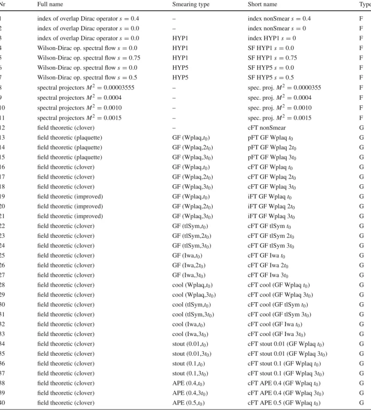
Table 2 The relevant characteristics of each topological charge defini- tion. For each definition, we give a number, full name, type of smear- ing of gauge fields (– = no smearing, HYPn =n iterations of HYP smearing, GF (action,t) = gradient flow with a given smoothing action (Wplaq = Wilson plaquette, tlSym = tree-level Symanzik improved, Iwa = Iwasaki) and at flow timet, cool (action,t) = cooling (smoothing action as for GF) and a number of steps corresponding to GF at flow

timet, stout (ρst,t) = stout smearing with a givenρst parameter and a number of steps corresponding to GF at flow timet, APE (αAPE,t)

= APE smearing with a givenαAPEparameter and a number of steps corresponding to GF at flow timet, HYP (t) = HYP smearing with a number of steps corresponding to GF at flow timet), short name (used in plots) and definition type (G=gluonic, F=fermionic)

Nr Full name Smearing type Short name Type

1 index of overlap Dirac operators=0.4 – index nonSmears=0.4 F

2 index of overlap Dirac operators=0.0 – index nonSmears=0 F

3 index of overlap Dirac operators=0.0 HYP1 index HYP1s=0 F

4 Wilson-Dirac op. spectral flows=0.0 HYP1 SF HYP1s=0.0 F

5 Wilson-Dirac op. spectral flows=0.75 HYP1 SF HYP1s=0.75 F

6 Wilson-Dirac op. spectral flows=0.0 HYP5 SF HYP5s=0.0 F

7 Wilson-Dirac op. spectral flows=0.5 HYP5 SF HYP5s=0.5 F

8 spectral projectorsM²=0.00003555 – spec. proj.M²=0.0000355 F

9 spectral projectorsM²=0.0004 – spec. proj.M²=0.0004 F

10 spectral projectorsM²=0.0010 – spec. proj.M²=0.0010 F

11 spectral projectorsM²=0.0015 – spec. proj.M²=0.0015 F

12 field theoretic (clover) – cFT nonSmear G

13 field theoretic (plaquette) GF (Wplaq,t0) pFT GF Wplaqt₀ G

14 field theoretic (plaquette) GF (Wplaq,2t0) pFT GF Wplaq 2t0 G

15 field theoretic (plaquette) GF (Wplaq,3t0) pFT GF Wplaq 3t0 G

16 field theoretic (clover) GF (Wplaq,t0) cFT GF Wplaqt₀ G

17 field theoretic (clover) GF (Wplaq,2t0) cFT GF Wplaq 2t0 G

18 field theoretic (clover) GF (Wplaq,3t0) cFT GF Wplaq 3t0 G

19 field theoretic (improved) GF (Wplaq,t0) iFT GF Wplaqt₀ G

20 field theoretic (improved) GF (Wplaq,2t0) iFT GF Wplaq 2t0 G

21 field theoretic (improved) GF (Wplaq,3t0) iFT GF Wplaq 3t0 G

22 field theoretic (clover) GF (tlSym,t0) cFT GF tlSymt₀ G

23 field theoretic (clover) GF (tlSym,2t0) cFT GF tlSym 2t0 G

24 field theoretic (clover) GF (tlSym,3t0) cFT GF tlSym 3t0 G

25 field theoretic (clover) GF (Iwa,t0) cFT GF Iwat₀ G

26 field theoretic (clover) GF (Iwa,2t0) cFT GF Iwa 2t0 G

27 field theoretic (clover) GF (Iwa,3t0) cFT GF Iwa 3t0 G

28 field theoretic (clover) cool (Wplaq,t0) cFT cool (GF Wplaqt₀) G

29 field theoretic (clover) cool (Wplaq,3t0) cFT cool (GF Wplaq 3t0) G

30 field theoretic (clover) cool (tlSym,t0) cFT cool (GF tlSymt₀) G

31 field theoretic (clover) cool (tlSym,3t0) cFT cool (GF tlSym 3t0) G

32 field theoretic (clover) cool (Iwa,t0) cFT cool (GF Iwat₀) G

33 field theoretic (clover) cool (Iwa,3t0) cFT cool (GF Iwa 3t0) G

34 field theoretic (clover) stout (0.01,t0) cFT stout 0.01 (GF Wplaqt₀) G

35 field theoretic (clover) stout (0.01,3t0) cFT stout 0.01 (GF Wplaq 3t0) G

36 field theoretic (clover) stout (0.1,t0) cFT stout 0.1 (GF Wplaqt₀) G

37 field theoretic (clover) stout (0.1,3t0) cFT stout 0.1 (GF Wplaq 3t0) G

38 field theoretic (clover) APE (0.4,t0) cFT APE 0.4 (GF Wplaqt₀) G

39 field theoretic (clover) APE (0.4,3t0) cFT APE 0.4 (GF Wplaq 3t0) G

40 field theoretic (clover) APE (0.5,t0) cFT APE 0.5 (GF Wplaqt₀) G

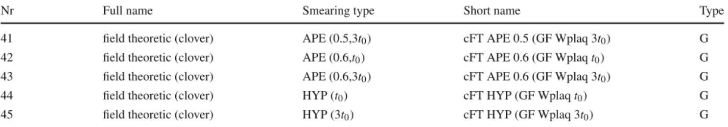
Table 2 continued

Nr Full name Smearing type Short name Type

41 field theoretic (clover) APE (0.5,3t0) cFT APE 0.5 (GF Wplaq 3t0) G

42 field theoretic (clover) APE (0.6,t0) cFT APE 0.6 (GF Wplaqt₀) G

43 field theoretic (clover) APE (0.6,3t0) cFT APE 0.6 (GF Wplaq 3t0) G

44 field theoretic (clover) HYP (t0) cFT HYP (GF Wplaqt₀) G

45 field theoretic (clover) HYP (3t0) cFT HYP (GF Wplaq 3t0) G

but at practically used lattice spacings, Q evaluated from the zero modes of the overlap operator shows a dependence on the value of the parameter s. In a sense, this reflects the general property that topology is uniquely defined only for continuum gauge fields. In Sect.

on the dependence of Q on s by explicitly comparing results obtained for different values of the latter.

The overlap index definition of the topological charge is theoretically clean and very appealing, because it provides integer values of Q, while for most other definitions dis- cussed in this paper, the Q values at non-zero lattice spacing are driven away from integers by cut-off effects, ultraviolet fluctuations and/or stochastic noise. However, it has a severe practical drawback – the cost of using the overlap operator is around one to two orders of magnitude larger than the one of e.g. variants of Wilson fermions [49].

3.2 Wilson-Dirac operator spectral flow

Closely related to the overlap index is the index derived from the spectral flow of the hermitian Wilson-Dirac operator [50,51]. Its definition is derived from the fact that the contin- uum hermitian Euclidean Dirac operator H

D(m

with bare mass m

0 has a gap, i.e. it has no eigenvalues in the region

m

m

. As a consequence, eigenvalues crossing zero in the spectral flow of H(m

can only occur at m

0, i.e. they correspond to the zero modes of D, and, hence, the net number of crossings is related to the topolog- ical charge of the background gauge field [45].

On the lattice, zero crossings in the spectral flow of the hermitian Wilson-Dirac operator H

m

can occur for any value of m

in the region

m

0 [52,53] and counting the net number of crossings in the region

s)

m

0 enables one to associate an index to the Wilson-Dirac operator as a function of s. The interpretation from the overlap formalism is essential to make this connection [51]. In fact, the correspondence between the index of the overlap operator and the index from the spectral flow is exact, so the parameter s in Eq. (5) is the same as the one used here, and all the good properties of the overlap index carry over to the index from the spectral flow.

To be more specific, we consider the hermitian Wilson- Dirac operator

H

m

(6) and its eigenvalues

m

defines the spectral flow. Since the Wilson-Dirac opera- tor D

is non-normal, the eigensystems of H

m

and D

m

are related in a non-trivial way, except for the modes of H

which are zero for a particular value of m

,

H

0

D

(7) It follows from this equation that the real modes

of D

correspond to zero modes of H

the chirality of the modes is given through first order per- turbation theory by the derivative of the spectral flow at m

[50],

d

dm

m₀=−λ_k^W

= k|γ5|k.

(8)

Finally, summing up the chiralities of the real modes

of D

up to 1

s yields an index of the Wilson-Dirac operator, and hence the topological charge from the spectral flow,

Q

λ^Wk ∈R

sign(k|γ

(9)

where the sum is over

1

s only, i.e. it excludes the real doubler modes.

Smoothing the gauge fields in the covariant derivatives of

D

reduces the non-normality of D

, and hence improves

the chirality of the real modes [47]. In addition, it also

improves the separation of the physical modes from the dou-

bler modes and in this way reduces the ambiguity of the

charge definition due to the choice of the parameter s. Inter-

estingly, this ambiguity can be quantified in the context of

Wilson Random Matrix Theory [54–58].

3.3 Spectral projectors

Another fermionic definition of the topological charge was introduced by Giusti and Lüscher [9,59]. One introduces the projector

to the subspace of eigenmodes of the squared Hermitian Dirac operator D

D with eigenvalues below M

. The projectors

can be evaluated stochastically and for chirally symmetric fermions, the topological charge can be defined in terms of it as Q

Tr

then equivalent to the index definition, apart from the fact that the counting of modes proceeds stochastically, instead of determining it from zero modes. For non-chirally symmet- ric fermions, the chirality of modes is no longer

can be schematically written as

1

a

. Thus, the above definition of Q still holds, but it gives in general non-integer values, contaminated by cut-off effects and by noise from the stochastic evaluation. In practice, the spectral projector com- putation of the topological charge proceeds in the following way for Wilson-type fermions [9]. One introduces in the the- ory a set

,

of N

pseudofermion fields with the action S

j=1(ηj, ηj), where the bracket denotes

the scalar product. The fields are generated randomly, thus their gauge ensemble average is distributed according to the introduced action. Then, one defines the observable

C=

1 N

N_{sr c}

j=1

PMηj, γ5PMηj

.

(10)

which plays the role of the topological charge. To compute the topological susceptibility from this definition, one needs a correction to account for a finite number of stochastic noise samples N

and the ratio of renormalization constants Z

. This is done using other observables

B=

1 N

Nsr c

j=1

PMγ5PMηj,PMγ5PMηj

,

(11)

A=

1 N

Nsr c

j=1

P²Mηj,P²Mηj

.

(12)

Then, the topological susceptibility,

1

V

C² − B

N

.

(13)

If the ratio Z

Z

is known from another computation, one can replace

in the above equation with Z

. We can, therefore, define as a proxy of the topological charge the quantity

Q

Z

Z

(14)

with Q

lim

Q

. It can be shown that the spectral projector definition is manifestly ultraviolet finite [11,59–

61] and hence theoretically very appealing, especially for

the computations of the topological susceptibility, as done in Refs. [9,60,62–65]. However, if the aim is to e.g. sepa- rate topological sectors, i.e. to choose configurations from a given sector, then the stochastic noise present in the spectral projector evaluated observables strongly contaminates the results, if using a relatively small N

6, while for large N

in the results section, the stochastic ingredient also makes the correlation with respect to other definitions only moder- ate and much smaller than e.g. the correlation between the field theoretic definitions (evaluated with different kinds of smearing).

The obtained result also depends on the spectral threshold M chosen for the projector

. As stated in Ref. [59], M can be chosen arbitrarily, but it is wise to avoid its large values in lattice units (that enhance cut-off effects) and also values close to the quark mass. We will check a few values of M and investigate the implications of choosing different values.

Recently, the spectral projector formalism was extended to staggered fermions [66]. In this case, the bare topological charge is also multiplicatively renormalizable, but the renor- malization constants are different, which is due to a different pattern of chiral symmetry breaking.

3.4 Field theoretic definition

The topological charge of a gauge field can be naturally defined as the four-dimensional integral over space-time of the topological charge density. In the continuum, this reads Q

d

x q(x), (15)

where q(x) denotes the topological charge density defined as

q

1

32

Tr

F

F

.

(16)

On the lattice, one has to choose a valid discretization q

of q

in order to evaluate Eq. (15), which now takes the form of the sum

Q

a

x

q

(17)

In practice, any discretization which gives the right contin-

uum limit can be used for the evaluation of Eq. (17), but

depending on the discretization q

ing the total topological charge Q can vary. This means that

using such an operator, on smoothed configurations as we

explain in Sect.

ger value for the total topological charge Q, but rather that

the obtained value of Q would be approaching an integer as

we tend to the continuum limit i.e. Q

integer

O(a

addition, we expect that the total topological charge for some definitions of q

converges faster and closer to an integer than that obtained by others. One can build such operators from closed path-ordered products of links which lead to the field strength tensor F

if we perturbatively expand them in a. Namely, by using a number of different Wilson loop shapes and sizes, we cancel, step by step, the leading lat- tice artifacts contributions. Examples of such operators are demonstrated in the next paragraph.

The simplest lattice discretization of q

is based on the simple plaquette and can be noted as

q

1

32π

Tr

C

C

,

(18)

with

C_μν^plaq(x) = Im

ˆ μ ˆ ν

,

(19) where the square pictorializes the path ordered product of the links lying along plaquette sides in the directions

and

ν

. This definition of q

x

has a low computational cost and leads to lattice artifacts of order

it has been used in several determinations of the topologi- cal susceptibility and investigations of the instanton proper- ties [67,68].

Without question, the most commonly used definition of q

is the symmetrized clover leaf noted as

q

1

32π

Tr

C

C

,

(20)

with

C_μν^clov(x) = 1 4Im

⎛

⎜⎝ ^μˆ

ˆ ν

⎞

⎟⎠.

(21) Like in the plaquette definition, clover includes lattice arti- facts of order

a

. This can be viewed easily by per- turbatively expanding C

x

and C

x

and obtaining 1

a

F

improved definitions of topological charge density operators by including additional Wilson loop shapes in the definition of q

and then perturbatively canceling the terms which contribute to higher powers of a. Such a definition is the Symanzik tree-level improved expressed as

q

x

b

q

x

b

q

x

(22) with

q

2

32π

Tr

C

C

,

(23)

and

C_μν^rect(x) =1 8Im

⎛

⎜⎜

⎜⎜

⎜⎝

ˆ μ ˆ ν

+ ^ˆμ

ˆ ν

⎞

⎟⎟

⎟⎟

⎟⎠ .

(24) q

is the clover-like operator where instead of squares we make use of horizontally and vertically oriented rectangu- lar Wilson loops of size 2

1. We remove the discretization errors at tree-level using the Symanzik tree-level coefficients b

and b

as these were previously used in Eq. (1). Thus, this definition of the topological charge density, by a semiclassi- cal inspection, converges as

a

in the continuum limit

. Hence, a way to obtain topological quantities with small lat- tice artifact contributions is by using improved topological density operators.

Ultraviolet fluctuations of the gauge fields entering in the definition of the topological charge density lead to contami- nation of the topological charge. Hence, we employ methods to suppress these UV fluctuations. Such techniques include the gradient flow, the extensively used cooling and several smearing schemes such as APE, HYP and stout. We exam- ine all the above smoothers and investigate their analytic as well as numerical relations.

It is worth mentioning that one can recover the correct definition of topological quantities from unsmoothed con- figurations by subtracting additive and multiplicative renor- malization constants at zero smoothing step. However, the extraction of these renormalization constants may be sub- ject to more systematic effects. Of course, this method is proven useful for particular studies such as the investigation of the

produced with the topological density weighted by an imag- inary theta term iθ being included in the QCD action [70].

Although this method of defining the topological charge is out of the scope of this work, the reader can find more infor- mation in Refs. [71] and [72].

3.5 Smoothing procedures

Smoothing a gauge link U

can be accomplished by its replacement by some other link that minimizes a local gauge action. To this purpose, it makes more sense to rewrite the

3 Other improved discretizations also exist, see e.g. Ref. [69].

4 An approach to reduce further the lattice artifacts and improve the convergence in the continuum limit is to shift the spikes of the topolog- ical charge distribution obtained with a given definition ofq_Laround exact integers. This has been introduced in Ref. [73] and used exten- sively since then. However, since this is a rather arbitrary redefinition of the topological charge, we omit its discussion in this manuscript.

lattice gauge action as S

3 ReTr{X

+{terms independent of

U

(25) where X

x

is the sum of all the path ordered products of link matrices, called the “staples”, which interact with the link U

components in X

x

are the staples extending over 1

1 squares (in lattice units). We can, therefore, write X

as X

x

ν≥0,ν=μ

U

x

U

x

a

U

x

a

U

a

a

a

a

.

(26) According to the above equation, for a given link U

the total number of plaquette staples interacting with it is 6. There are several ways to iteratively minimize the local action. These include procedures such as the gradient flow, cooling, APE and stout smearing, which make use of the original staples X

to minimize the local action; this pro- vides the opportunity to perturbatively relate these smoothers and obtain a more concrete understanding on the numerical equivalence among them. Furthermore, other more sophis- ticated smearing procedures such as HYP smearing, which makes use of a more complicated construction of staples, also exist. However, the latter, although it leads to numer- ical equivalence with the other smoothing techniques, pro- hibits us from relating it perturbatively at tree-level order with other smoothing techniques. In the next subsections, we give a brief overview of these most commonly used smoothing techniques used for the calculation of the topological charge.

3.5.1 Gradient flow

Modern non-perturbative studies of QCD have been employ- ing the gradient flow, which has been proven to be a pertur- batively and numerically well-defined smoothing procedure.

It has good, perturbatively proven renormalization proper- ties and the fields which have been smoothed via gradient flow do not need to be renormalized. From a historic point of view, the gradient flow is related to the streamline idea of Refs. [74–76] and its lattice counterpart was previously introduced in the context of Morse theory [77].

The gradient flow is defined as the solution of the evolution equations [12–16]

V

∂x,μ

S

V

V

x

0

U

x

(27)

where

is the dimensionless gradient flow time. In the above equation, the link derivative is defined as

∂x,μ

S

i

a

T

d ds S

e

U

≡

i

a

T

S

U

(28) with

Y

T

if

0 if

(29)

and T

(a

1,

8) the Hermitian generators of the SU(3) group. If we now set

U

obtain

g

S

1 2

Ω_μ(x)−Ω_μ^†(x)

−

1 6 Tr

Ω_μ(x)−Ω_μ^†(x)

.

(30)

The last equation provides all we need in order to smooth the gauge fields according to the Eqs. (27). Evolving the gauge fields via the gradient flow requires the numerical integra- tion of Eqs. (27) manifested by an integration step

. This is performed using the third order Runge-Kutta scheme, as explained in Ref. [16]. We set

0.01 for the integration step, since this has been shown to be a safe option [18]. For the exponentiation of the Lie-algebra fields required for the integration, we apply the algorithm described in Ref. [78].

An important use of the gradient flow is the determination of a reference scale t

, defined as the gradient flow time t

a

in physical units for which

t

E(t)|

0.3, (31)

where E

t

is the action density E

1

2V

x

Tr

F

t

t)

.

(32)

To evaluate numerically E

tion similarly to Eq. (20).

Having defined the reference scale t

, a question is raised:

for what value of t shall we read an observable? It has been argued that cut-off effects in some observables can be reduced by chosing larger flow times as reference length scales [79,

of the topological charge obtained with gradient flow with that extracted using different smoothers for three different gradient flow times, namely, t

, 2t

and 3t

.

3.5.2 Cooling

The smoothing technique of cooling [81–84] was one of the

first methods used to remove ultraviolet fluctuations from

gauge fields. Cooling is applied to a link variable U

SU

3

by updating it, from an old value U

x

to U

x

, according to the probability density

P(U)

exp

−

lim

β→∞β

1

3 ReTrX

.

(33)

The basic step of the cooling algorithm is to replace the given link U

by an SU

group element, which minimizes locally the action, while all the other links remain untouched.

This is done by choosing a matrix U

x

SU

3

that maximizes

ReTr{U

(34)

In the case of an SU(2) gauge theory, the maximization is achieved by

U

X

det X

x

(35)

For SU

Cabibbo-Marinari algorithm [85] according to which one has to iterate the maximization over all the SU

subgroups embedded into SU

We iterate this procedure so that all the links on all sites are updated. Such a sweep over the whole lattice is called one cooling step n

1. Traditionally, during such a sweep the link variables, which have already been updated, are subse- quently used for the update of the links still retaining their old value. Nevertheless, one can also consider to use the updated links only after the whole lattice is covered, increasing the CPU time by a factor of two.

3.5.3 APE (Array Processor Experiment) smearing An alternative way to smooth the gauge fields is to apply APE smearing [86] on the gauge configurations. According to this smoothing procedure, we create fat links by adding to the original links the neighbouring staples weighted by a rel- ative strength

, which represents the smearing fraction and can be tuned according to its use. This operation breaks unitarity of the resulting “fat” links and shifts them away from det U

1, thus, we should project back to SU

above operation is noted as

U

Pr oj

(1−αAPE)

U

6 X

x

.

(36)

The APE smearing scheme can be iterated n

times to produce smeared links. In addition to the simple APE smear- ing, variations which make use of “chair” and “diagonal”

staples have been proposed from time to time. For the pur- poses of this investigation, we have considered just the simple

APE smearing for different values of the

parameter:

αAPE=

0.1, 0.2, 0.3, 0.4, 0.5 and 0.6. (37) One can project back to SU(3) by maximizing the expres- sion ReTr

U

x

X

x

with U

x

being the unprojected smeared link. Nonetheless, one can project onto SU(3) using other iterative procedures which suggest that there is not a unique way to do so. This subtlety, however, becomes irrelevant in analytic smearing schemes such as the stout.

3.5.4 Stout smearing

A method which allows analytical derivation of smoothed configurations in SU(3) is the so–called stout smearing pro- posed in Ref. [78]. This smoothing scheme works in the fol- lowing way. Once again, let X

denote the weighted sum of the perpendicular staples which begin at lattice site x and terminate at neighboring site x

a

. Now, we give a weight

to the staples according to

C

X

(38)

The weight

is a tunable real parameter. Then, the matrix Q

SU

by

Q

i 2

Ξ_μ^†(x)−Ξ_μ(x)

−

i 6 Tr

Ξ_μ^†(x)−Ξ_μ(x)

(39) is Hermitian and traceless, where

Ξμ(

x

C

x

U

x

(40) Thus, we define an iterative, analytic link smearing algorithm in which the links U

x

at stout smearing step n

are mapped into links U

at stout smearing step n

1 using

U

exp

i Q

U

(41) This step can be iterated n

times to finally produce link vari- ables in SU(3) which we call stout links. The structure of the stout smearing procedure resembles the exponentiation steps of the gradient flow and, as a matter of fact, the gradient flow using the Wilson gauge action can be considered as a con- tinuous generalization of stout smearing [87], using gauge paths more complicated than just staples. Hence, for a small enough lattice spacing, one would expect the two smoothing schemes to provide extremely similar results. The level of this similarity is investigated in this work.

3.5.5 HYP (Hypercubic) smearing

We turn now to the discussion of the HYP (Hypercubic)

smearing which has been introduced in Ref. [88]. The

smeared links of the HYP smoothing procedure are con- structed in three steps. These steps are described in the next bullet points.

3. The final step of the HYP smearing consists of applying an APE smearing routine in which the staples are con- structed by decorated links which have undergone HYP smearing levels 1 and 2:

U

Pr oj

X

(42) with

X

ν≥0,ν=μ

U

U

a

U

a

+ ˜

U

a

U

(x−

a

U

a

a

.

(43)

The link U

is the original link in

direction which has been smoothed n

times. U

x

are fat links along the direction

resulting from the second step of the HYP smearing procedure with the staples extend- ing over direction

being not smeared. The parameter

is tunable and real.

2. The second step of HYP smearing creates the decorated links U

x

by applying a modified APE smearing pro- cedure according to

U

Pr oj

4 X

(44)

with X

=

ρ≥0,ρ=ν,μ

U

a

a

+U^†_ρ;ν,μ(x−

a

U

a

a

a

(45) Once more, the link U

is the link in

direction which has been smoothed n

times. Now, U

are fat links along direction

resulting from the first step of the HYP smearing procedure with staples extending in the directions

being non smeared. The parameter

is again tunable and real.

1. The decorated links U

are built from the links which have been smeared n

using the modified APE smearing step:

U

x

Pr oj

(

1

U

x

+α2

2 X

x

,

(46)

with X

=

σ≥0,σ=ρ,ν,μ

U

x

U

x

a

U

a

+U^†(_σⁿ_;ρ,ν,μ^HYP) (x−

a

a

U

a

a

.

(47)

In the above expression, only the two staples orthogonal to directions

are included in the smearing proce- dure.

For the purpose of our work, we choose the values [88]

α1=

0

75

0

6

0

3

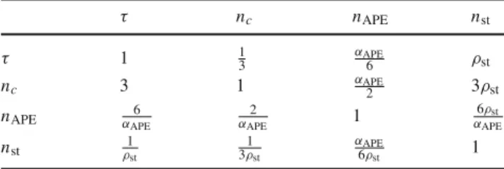
(48) 3.5.6 Perturbative relation between smoothing techniques The gradient flow, cooling as well as APE, stout and HYP smearing schemes can be used to remove the ultraviolet fluc- tuations and should lead to the same topological properties, provided that we are close enough to the continuum limit.

Assuming that a is small enough so that we are in the per- turbative regime, we can carry out a comparison between the different smoothing procedures in order to obtain an analytic relation among the associated smoothing scales involved, fol- lowing Refs. [18,19]. Since the gradient flow has the advan- tage of being the only smoothing scheme with good, pertur- batively proven, renormalizability properties, we first relate all other smoothing schemes with the gradient flow and, sub- sequently, with each other.

Gradient flow. The perturbative investigation of the relation between the gradient flow using the Wilson action and cool- ing has been studied in Ref. [18]. The authors demonstrated that the two smoothing schemes alter the links of a gauge configuration by the same amount if one rescales the flow time and the number of cooling steps according to

τ

n

3

(49)

In the following few lines, we sketch the extraction of the derivative evolution of a gauge link in order to compare it to other smoothing schemes.

In the perturbative regime, a link variable which has been smoothed via the Wilson flow

for a finite flow time

can be expanded as

U

x

11

i

a

u

x

T

(50) with u

assumed to be infinitesimal. Using Eq. (26), the plaquette staples are written as

X

6

11

i

a

w^a_μ(x, τ)T^a,

(51) where

is an infinitesimal quantity. The leading coef- ficient with the value 6 appearing in the above equation is just the number of plaquettes interacting with the link on which the Wilson flow evolution is applied. We can, therefore, write

as

Ω_μ(x, τ)

6

11

a

6u

T

(52) Hence, Eq. (30) becomes

g

S

i

a

6u

T

(53) Using the above expression, the evolution of the gradient flow by an infinitesimally small flow time

can be approximated as

u

u

6u

(54) Since the gradient flow is the only smoothing scheme with a concrete theoretical foundation and good renormalizability properties, we will attempt to relate it to other smoothing schemes. Hence, through the resulting matching formulae of any smoothing technique with the gradient flow, we will be able to relate all the different smoothing schemes with each other.

Cooling In the cooling procedure, the link U

n

is sub- stituted with the projection of X

n

over the gauge group. Namely, for the case of the SU

2

gauge theory, this projection is manifested by Eq. (35) where we substitute X

n

by Eq. (51). In the perturbative approximation, this leads to

U

11

i

a

w^a_μ(

x

n

6 T

(55)

5For convenience, here and in the following we refer to the gradient flow using the Wilson gauge action in short as the ’Wilson flow’. This is not to be confused with the spectral flow of the Hermitian Wilson Dirac operator which in the past sometimes has also been called ’Wilson flow’.

The above update corresponds to the substitution u

n

1)

x

n

6

(56)

Comparing Eqs. (54) and (56), one sees that the flow would evolve the same as cooling if one chooses a step of

1/6.

In addition, during a whole cooling step, the link variables which have already been updated are subsequently used for the update of the remaining links that await update; this cor- responds to a speed-up of a factor of two. Therefore, the predicted perturbative relation between the flow time

and the number of cooling steps n

so that both smoothers have the same effect on the gauge field is given by Eq. (49). This has been shown analytically and demonstrated numerically in Ref. [18]. Moreover, the authors in Ref. [19] have gener- alized this equivalence for the case of the gradient flow and cooling employing smoothing actions which in addition to the square term multiplied by a factor of b

, also included a rectangular term multiplied by b

b

alence in manifested by the formula

τ

n

3

15b

(57)

In Sect.

for the Wilson smoothing action is manifested by Eq. (49).

APE smearing. We now move to the case of the APE smear- ing and relate it perturbatively to the Wilson flow and con- sequently to cooling and stout smearing. Once more, we express the gauge link U

n

in terms of elements of its Lie algebra

U

x

11

i

a

u

x

n

T

(58) Subsequently, we apply this expansion to Eq. (36) and obtain the evolution equation

u

n

1) u

n

−αAPE

6

6u

n

n

.

(59)

Comparing Eqs. (54) and (59), we observe that the Wilson flow would evolve the gauge links the same as APE smear- ing if one chooses a flow step of

perturbative relation between the Wilson flow time

and the number of APE smearing steps n

so that both smoothers have the same effect on the gauge field is

τ =αAPE

6 n

(60)

The above perturbative matching relation is investigated numerically in Sect.

Stout smearing. Let us now turn to the stout smearing smooth-

ing procedure and check whether we could demonstrate ana-

lytic equivalence with the Wilson flow and consequently with