ATLAS-CONF-2010-050 28July2010
ATLAS NOTE
ATLAS-CONF-2010-050
July 16, 2010
Measurement of jet production in proton-proton collisions at 7 TeV centre-of-mass energy with the ATLAS Detector
The ATLAS Collaboration
Abstract
Jet cross sections have been measured with the ATLAS detector for the first time in proton-proton collisions at centre-of-mass energy of 7 TeV, using an integrated luminosity of 17 nb−1. The anti-k⊥ algorithm is used to identify jets, using two jet radius parameters, R=0.4 and 0.6. Inclusive single-jet differential cross sections are presented as functions of jet transverse momentum and rapidity. Dijet cross sections are presented as functions of dijet mass and angle. The results are compared to expectations based on next-to-leading- order QCD, which agree with the data.
1 Introduction
At the Large Hadron Collider (LHC), jet production is the dominant high transverse-momentum (pT) process and as such gives the first glimpse of physics at the TeV scale.
Jet rates and cross sections are key observables in high-energy particle physics. They have been measured in e+e−, ep, pp and pp¯ colliders, as well as in γp andγ γ collisions. They have provided precise measurements of the strong coupling constant, have been used to obtain information about the structure of the proton and photon, and have become an important tool for understanding the strong interaction and searching for physics beyond the Standard Model (see, for example, [1]). In this note, we present the first measurements of inclusive single-jet and dijet cross sections using the ATLAS detector.
The measurements are performed using data taken between 30 March and 5 June 2010, when the LHC delivered proton-proton collisions at a centre-of-mass energy √
s=7 TeV. The data correspond to an integrated luminosity of 17±2 nb−1. The integrated luminosities are calculated run-by-run by measuring data rates in several ATLAS sub-components at low angles to the beam direction, with the absolute calibration obtained from a Van der Meer scan [2].
1.1 Cross Section Definition
Jets are identified using the anti-k⊥jet algorithm [3]. This algorithm constructs, for each input objecti, the quantitiesdi j anddiBas follows:
di j = min(k−2⊥i,k−2⊥j)(∆R)2i j
R2 (1)
diB = k−2⊥i, (2)
where
(∆R)2i j= (yi−yj)2+ (φi−φj)2, (3) k⊥iis the transverse momentum of objectiwith respect to the beam direction,φi is its azimuthal angle, andyi is its rapidity, defined asy= 12ln[(E+pz)/(E−pz)], where E denotes the energy and pz is the component of the momentum along the beam direction. A list containing all the di j anddiB values is compiled. If the smallest entry is adi j, objectsiand jare combined and the list is remade. If the smallest entry is adiB, this object is considered a complete “jet” and is removed from the list. As defined above,di j is a distance measure between two objects, anddiBis a similar distance between the object and the beam.
Thus the variableRis a resolution parameter which sets the relative distance at which jets are resolved from each other as compared to the beam. In this analysis, two different values for theRparameter are chosen: R=0.6 andR=0.4. The anti-k⊥ algorithm is well-motivated since it can be implemented in NLO QCD calculations and produces geometrically well-defined (“cone-like”) jets.
The measurements are corrected for all experimental effects, and so refer to the ideal “truth” final- state of a proton-proton collision, where particles with a lifetime longer than 10ps are considered stable.
This definition includes muons and neutrinos from hadronic decays (see, for example [4]).
Kinematic variables are defined in the ATLAS reference system, which is a Cartesian right-handed coordinate system, with nominal collision point at the origin.1
Inclusive single-jet double-differential cross sections are measured as a function of jet pT andy in the regionpT>60 GeV,|y|<2.8. This ensures that jets lie well within the high efficiency plateau region for the triggers used, as described in Section 5.1, and that the jets are in a region where the energy scale is well understood, as described in Section 5.2.
1The anti-clockwise beam direction defines the positivez-axis, with thex-axis pointing to the centre of the LHC ring.
Dijet double-differential cross sections are measured as a function of the dijet mass,m12, binned in the maximum rapidity of the two leading jets,|y|max=max(|y1|,|y2|); and of the angular variable
χ=exp(|y1−y2|)≈ 1+cosθ∗
1−cosθ∗ (4)
binned in the dijet massm12. Herey1corresponds to the highestpTjet in the event andy2to the second highest, andθ∗is the polar scattering angle in the dijet centre-of-mass frame. The leading jet is required to lie in the pT,|y|kinematic region defined above. The subleading jet is required to lie in the same rapidity region and to have pT >30 GeV. Allowing the second jet to extend to lower pT improves the stability of the next-to-leading-order (NLO) calculation [5]. Again, the pT >60 GeV cut on the leading jet ensures that the jet trigger efficiency is high, while the pT>30 GeV cut on the subleading jet ensures that both the jet reconstruction efficiency and purity are above 99%. The subleading jet pT cut is also important to limit misidentification of the subleading jet due to poor jet energy resolution for
pT<30 GeV (see Section. 5.4).
The dijet mass is plotted in the allowed rapidity region only above the minimum mass where it is no longer biased by thepT and rapidity cuts on the two leading jets. The minimum unbiased mass depends on the|y|maxbin, which determines the maximum opening angle in rapidity allowed. The biased spectrum below this mass is not measured due to its particular sensitivity to the jet energy scale uncertainty through the jet pTcut.
The χ =exp(|y1−y2|) angular variable is plotted up to maximum of 30, restricting the angular separation in rapidity to |y1−y2|<log(30). In the rotated coordinate system (y∗, yboost), wherey∗ is related to the scattering angle in the dijet centre-of-mass system andyboost=0.5(y1+y2)is the boost of the dijet system with respect to the lab frame, this restricts the acceptance to |y∗|<0.5×log(30). An orthogonal acceptance cut |yboost|<1.1 is then made on the χ distribution in order to reject events in which both jets are boosted into the forward or backward hemisphere. This reduces the sensitivity to parton density function (PDF) uncertainties at lowxand in turn enhances sensitivity to differences that could arise from deviations from the matrix element predictions of perturbative QCD. Theχ spectrum is plotted only in mass bins above the minimum mass where the mass becomes unbiased by the cuts on minimum jet pTand maximum opening angle|y1−y2|=log(30)between the two leading jets.
2 The ATLAS Detector and Simulation
The ATLAS detector covers nearly the entire solid angle around the collision point with layers of tracking detectors, calorimeters, and muon chambers. For the measurements presented in this note, the inner tracking devices, the calorimeters, and the trigger are of particular importance. These components, and the rest of the detector, are described in detail elsewhere [6].
The ATLAS inner detector has full coverage inφ and covers the pseudorapidity2range|η|<2.5. It consists of a silicon pixel detector, a silicon microstrip detector, and transition radiation tracker immersed in a 2 Tesla magnetic field. These tracking detectors are used to reconstruct tracks and vertices, including the primary vertex.
High granularity liquid-argon (LAr) electromagnetic sampling calorimeters, with excellent energy and position resolution performance, cover the pseudo-rapidity range|η|<3.2. The hadronic calorime- try in the range |η|<1.7 is provided by a scintillator-tile calorimeter, which is separated into a large barrel (|η|<1.0) and two smaller extended barrel cylinders, one on either side of the central barrel (0.8<|η|<1.7). In the end-caps (|η|>1.5), LAr hadronic calorimeters match the outer|η|limits of
2Pseudorapidity rather thanyis used for calibrations based on detector geometry, and is defined asη=−ln(tan(θ/2)), where the polar angleθis taken with respect to the positivezdirection. For massless objects, it is equivalent to rapidity.
the end-cap electromagnetic calorimeters. The LAr forward calorimeters provide both electromagnetic and hadronic energy measurements, and extend the coverage to|η|<4.9.
The ATLAS Trigger system uses three consecutive trigger levels to select signal events and reject background events. The Level-1 trigger is based on custom-built hardware to process the incoming data with a fixed latency of 2.5µs. This is the only trigger level used in this analysis. In order to commission the trigger software, the higher level triggers also recorded decisions on events, but these decisions were not applied to reject any data. The events in this analysis were accepted either by the system of minimum-bias trigger scintillators (MBTS) or the calorimeter trigger.
The MBTS detector [7] consists of 32 scintillator counters that are each 2 cm thick, which are orga- nized into two disks with one on each side of the ATLAS detector. The scintillators are installed on the inner face of the end-cap calorimeter cryostats at z=±3560 mm such that the disk surface is perpen- dicular to the beam direction. This leads to a coverage in|η|of 2.09 to 3.84. The MBTS multiplicity is calculated for each side independently, and allows events containing jets to be triggered with high efficiency and negligible bias.
The Level-1 calorimeter trigger uses coarse detector information to identify the position of interesting physics objects above a given energy threshold. The ATLAS jet trigger is based on the selection of jets according to their transverse energy,ET. The Level-1 jet reconstruction uses so-called jet elements, which are formed from the electromagnetic and hadronic calorimeters with a granularity of∆φ×∆η=0.2×0.2 for|η|<3.2. The jet finding is based on a sliding window algorithm with steps of one jet element, and the jetETis computed in a window of configurable size around it.
Both data and simulated events are fully reconstructed offline, using objected-oriented analysis soft- ware running on a distributed computing grid.
3 Monte Carlo Samples
Samples of simulated jet events in proton-proton collisions at√
s=7 TeV were produced using several Monte Carlo generators. The Pythia 6.421 [8] event generator is used for the baseline comparisons and corrections. This implements leading-order (LO) perturbative QCD matrix elements for 2→2 processes, parton showers calculated in a leading-logarithmic approximation, an underlying event3simulation using multiple-parton interactions, and uses the Lund string model for hadronisation. For studies of systematic variations, jet samples were produced using the Herwig 6 [9] generator, which also employs LO pQCD matrix elements, but uses an angle-ordered parton shower model and a cluster hadronisation model. The underlying event for the Herwig 6 samples is generated using the Jimmy [10] package, which again generates multiple-parton interactions. The Herwig++ [11], AlpGen [12] , and Sherpa [13] programmes were also used for various cross-checks.
The samples are created using a special tuned set of parameters denoted as ATLAS MC09 [14] with MSTW LO∗[15, 16] PDFs, unless stated otherwise.
The generated four-vectors are passed through a full simulation [17] of the ATLAS detector and trigger based on GEANT4 [18]. Finally, the events are reconstructed and selected using the same analysis chain as for the data with the same trigger, jet and event selection criteria.
4 Theoretical Predictions
Several NLO QCD calculations for jet production in proton-proton collisions are available. For compar- ison with our data we have used NLOJET++ 4.1.2 [19], with JETRAD [20] being used for cross-checks.
3The term underlying event is used to mean particles produced in the same proton-proton collision, but not originating from the primary hard partonic scatter or its products.
The CTEQ 6.6 [21] NLO parton densities were used for the central value, with the MSTW 2008 [15], NNPDF 2.0 [22], and HERAPDF 1.0 [23] parton density sets being used to evaluate the uncertainties. To estimate the potential impact of higher order terms not included in the calculation, the renormalisation scale was varied from a half to twice the default scale. To estimate the impact of choice of scale where the PDF evolution is separated from the matrix element, the factorisation scale was similarly varied.
These two scales were varied independently apart from a constraint that the ratio of the two scales be between 12 and 2, applied to avoid introducing large logarithms of the ratio of the scales. In addition, the uncertainty in the measurement of the strong coupling constant,αs(MZ), was estimated by calculating the cross section using αs(MZ) values within the uncertainty range, and using PDFs fitted using these values. To efficiently calculate all these uncertainties, the APPLgrid [24] program was used.
The NLO calculations predict partonic cross sections, which are unmeasurable. For comparison with data at the particle-level, soft (non-perturbative) corrections must be applied. This was done using leading-logarithmic parton showers, by evaluating the ratio of the cross section before hadronisation and underlying event compared to the cross section after it, and dividing the NLO theory distributions by this factor. The Pythia 6 and Herwig 6 models described above were used, as well as a variety of alternative tunes of Pythia 6 [25] as a cross-check. The soft QCD corrections depend signficantly on the value of R (0.4 or 0.6). The central value used is that from the Pythia 6 MC09 sample, and the uncertainty is estimated as the maximum spread of the other models investigated. To calculate the particle and parton level theory distributions, the Rivet [26] package was used.
5 Data Selection and Calibration
5.1 Trigger
The MBTS 1 trigger, which requires a single counter over threshold, was operated early in the data- taking period. It was used to trigger approximately 2% of the integrated luminosity of the data sample analysed. It has negligible inefficiency (measured in data with respect to random triggers [7]) for the events considered in this analysis, which all contain several charged tracks. As the instantaneous lumi- nosity increased, this trigger had a large prescale applied so subsequent events – comprising approxi- mately 98% of the data sample studied – were triggered by the jet trigger.
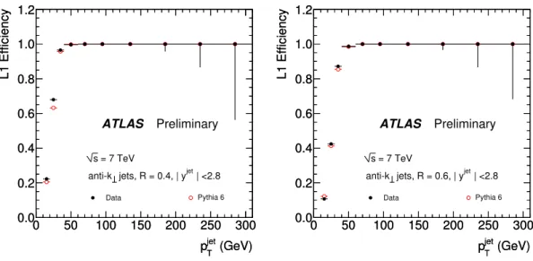
The lowest threshold jet trigger, L1 J5, uses a 0.4×0.4 window size in η−φ and requires a jet with pT >5 GeV at the “electromagnetic scale”4. The inclusive jet trigger efficiency for L1 J5 was measured with respect to the MBTS 1 trigger, which as described above provides an unbiased reference.
Its efficiency is shown as a function of the final reconstructed pT for single jets (R=0.4 and 0.6) in Fig. 1. The efficiency is compared to that predicted from Monte Carlo, demonstrating that the modelling of the trigger efficiency curve is good. The trigger efficiency for jets with pT>60 GeV and|y|<2.8 is above 99%. All events considered here contain at least one jet in this region.
5.2 Jet Energy Scale Calibration
The input objects to the jet algorithm in the data and in the detector-level simulation are topological calorimeter clusters [27]. The baseline calibration for these clusters, taken from test-beam measurements, corrects the cluster energy to the electromagnetic energy scale. After a jet is identified, its energy needs to be further calibrated to account for the fact that the ATLAS calorimeter has a lower response to hadronic energy than to electromagnetic energy, and for the fact that there is material in front of the calorimeter that absorbs some of the energy of the original particles. The jet energy calibration is carried out in bins ofηandpTand is based upon Monte Carlo simulation, the relevant properties of which have been shown
4“Electromagnetic scale” is the calibrated scale for energy deposited by electrons and photons in the calorimeter.
(GeV)
jet
pT
0 50 100 150 200 250 300
L1 Efficiency
0.0 0.2 0.4 0.6 0.8 1.0 1.2
Data Pythia 6
Data Pythia 6
ATLAS Preliminary
= 7 TeV s
| <2.8 jets, R = 0.4, | yjet
anti-k
(GeV)
jet
pT
0 50 100 150 200 250 300
L1 Efficiency
0.0 0.2 0.4 0.6 0.8 1.0 1.2
(GeV)
jet
pT
0 50 100 150 200 250 300
L1 Efficiency
0.0 0.2 0.4 0.6 0.8 1.0 1.2
Data Pythia 6
Data Pythia 6
ATLAS Preliminary
= 7 TeV s
| <2.8 jets, R = 0.6, | yjet
anti-k
(GeV)
jet
pT
0 50 100 150 200 250 300
L1 Efficiency
0.0 0.2 0.4 0.6 0.8 1.0 1.2
Figure 1: Inclusive jet trigger efficiency as a function of reconstructed jet pTfor jets identified using the anti-k⊥algorithm with (left)R=0.4 and (right)R=0.6.
to give an adequate description of the data. Test-beam data [28, 29] and in-situ measurements [30, 31]
show that the detector simulation models the calorimeter response to single hadrons to within 5%.
The final energy scale calibration and its estimated uncertainty account for uncertainties in the mod- eling of hadronic showers in the detector, the description of calorimeter noise, the material in front of the calorimeter, and uncertainties in the translation of the test-beam energy scale to the in-situ calorimeter. In the later data-taking periods used here, the effects of pile-up (multiple proton-proton interactions) were small, but not negligible, and are also accounted for in this uncertainty. Finally, the model-dependent uncertainty due to the hadronisation, parton shower and underlying event models is estimated by com- paring the correction derived using a sample of Pythia 6 events to that derived using a sample of AlpGen +Herwig 6 +Jimmy events, and is found to be below 3%.
The size of the overall correction to the pT of the jets is below 50%, and for central jets (i.e. jets in the barrel region) with pT>60 GeV it is around 35%. The overall uncertainty is below 9% over the entire range of pT andyconsidered, and below 7% for central jets with pT>60 GeV. The response as a function ofη is understood and modelled to within 5% for|η|<2.8 [32]. Full details of the energy scale evaluation are given elsewhere [33].
5.3 Analysis Selection Criteria
The jet algorithm is run on calorimeter clusters assuming that the event vertex is at the origin. The jet momenta are then corrected using the primary vertex position. After calibration, all events are required to have at least one jet within the kinematic region pT>60 GeV,|y|<2.8. Additional quality criteria are also applied to ensure that jets are not produced by single noisy calorimeter cells nor problematic detector regions [34]. Events are required to have at least one vertex consistent with the beamspot position, with at least five tracks connected to it, and with |z|<10 cm. The z vertex distribution in the simulation is reweighted to agree with that in the data. The overall efficiency of these selection cuts, evaluated in simulation using events with true particle-level jets in the kinematic region of the measurement and which pass the trigger, is above 99%, and has a small dependence on the kinematic variables. Background contributions from non-pp-collision sources were evaluated using unpaired and empty bunches and found to be negligible.
After this selection, 56535 (77716) events remain with at least one jet passing the inclusive jet selec- tion, and of these, 45621 (65739) events pass the dijet selection, forR=0.4(0.6).
5.4 Data Correction
The correction for all trigger and detector efficiencies and resolutions, other than the energy scale correc- tion already applied, is performed in a single step using a bin-by-bin migration function evaluated using the validated MC samples. For each measured distribution, the MC final-state-particle cross section is evaluated in the relevant bins, along with the equivalent distributions as seen in the simulated detector.
The ratio of the distributions provides a correction factor which is then applied to the data as seen in the detector.
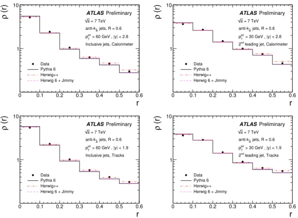
This procedure is justified by the good modelling of the trigger efficiencies (Fig. 1) and the fact that the pT and y distributions of the jets are reasonably well described by the simulation [32]. It is also important that the energy flow around the jet core is well understood. The energy and momentum flow within jets can be expressed in terms of the differential jet shape, defined as the fraction,ρ, of the jet momentum contained within a ring of thickness∆r=0.1 at a radiusr=p
(∆η)2+ (∆φ)2 around the jet centre, divided by∆r. The uncorrected jet shapes measured using calorimeter clusters and tracks are shown separately in Fig. 2 for anti-k⊥ jets withR=0.6. The jets simulated by Pythia 6 are slightly narrower than the jets in the data, while the Herwig 6 +Jimmy and Herwig++ simulations provide a better description. Overall the distribution of energy within the jets is reasonably well simulated. A similar level of agreement has been demonstrated forR=0.4 jets. This gives further confidence in the calibrations and corrections applied.
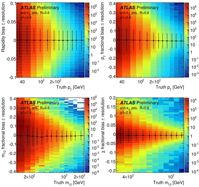
The resolutions iny, pT, dijet mass m12, and dijet χ for anti-k⊥ jets withR=0.6 within|y|<2.8 are shown in Fig. 3 as obtained using Pythia 6 Monte Carlo. From dijet balance and E/p studies of single hadrons, the pT resolution has been verified to within ≈ 14% [35], though at a lower pT than most of the jets considered here. The effect of varying the nominal pT resolution by up to 15% is included in the systematic uncertainty on the unfolding correction factors. The uncertainties due to jet energy scale are also propagated through to the final cross section through this unfolding procedure, by applying variations to simulated samples. The effects of pile-up on the energy measurement, weighted appropriately by luminosity, are also accounted for in this step. The final systematic uncertainty is completely dominated by the jet energy scale uncertainty.
The overall correction factor for thepTspectrum is below 20% throughout the kinematic region, and for central jets with pT>60 GeV is below 10%. For the dijet mass spectrum, the correction factors are generally within 15% while forχ the corrections are less than 5%.
6 Results and Discussion
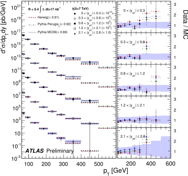
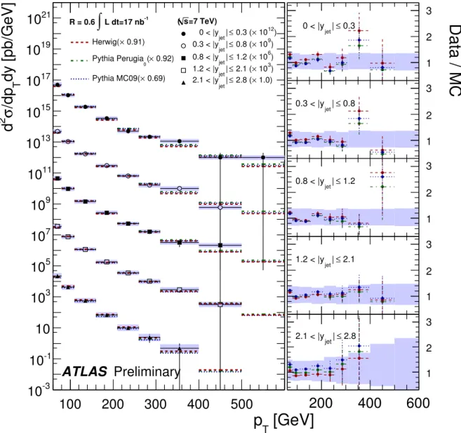
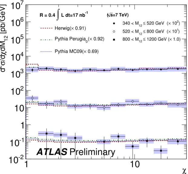
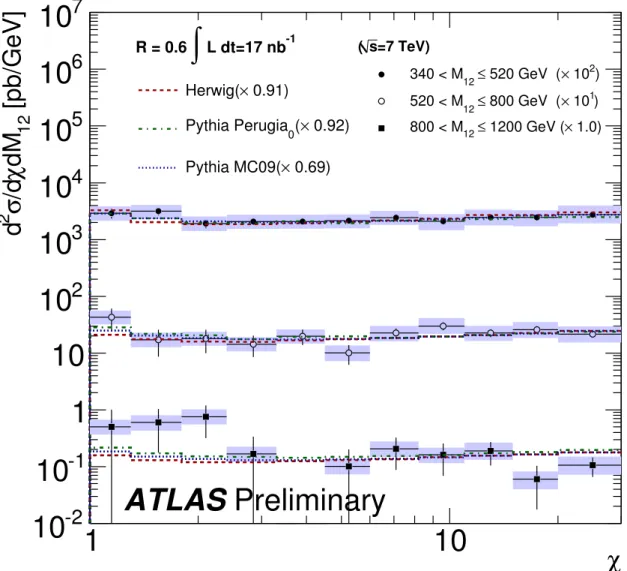
The normalisation of the leading-logarithmic parton-shower Monte Carlo generators is not reliable, since it is a leading-order calculation. However, a comparision of the shapes of the distributions is valuable, since many important kinematic terms are included and the predictions are made at particle-level. The expectations for the corrected pT andχ distributions from two different Pythia 6 parameter settings, as well as for Herwig 6 +Jimmy programs are compared to the data in Figs. 4, 5, 6 and 7. The normalisation of the Monte Carlo is to the average of theR=0.4 andR=0.6 cross sections, and requires the factors shown in the legend. In general the simulations agree with the shapes of the data distributions.
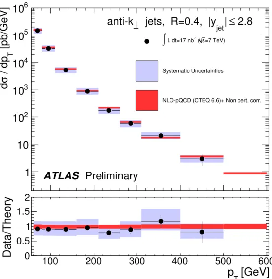
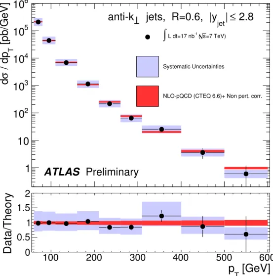
The differential inclusive-jet cross section in 7 TeV proton-proton collisions is shown in Fig. 8 and Fig. 9 as a function of jet pT, for anti-k⊥ jets withR=0.4 andR=0.6 respectively. The cross section extends frompT=60 GeV up to aroundpT=600 GeV, and falls by more than four orders of magnitude
r
0 0.1 0.2 0.3 0.4 0.5 0.6
(r)ρ
1 10
ATLASPreliminary = 7 TeV
s
Data Pythia 6 Herwig++
Herwig 6 + Jimmy
jets, R = 0.6 anti-k
> 60 GeV , |y| < 2.8
jet
pT
Inclusive jets, Calorimeter
r
0 0.1 0.2 0.3 0.4 0.5 0.6
(r)ρ
1 10
ATLASPreliminary = 7 TeV
s
Data Pythia 6 Herwig++
Herwig 6 + Jimmy
jets, R = 0.6 anti-k
> 30 GeV , |y| < 2.8
jet
pT
leading jet, Calorimeter 2nd
r
0 0.1 0.2 0.3 0.4 0.5 0.6
(r)ρ
1 10
ATLASPreliminary = 7 TeV
s
Data Pythia 6 Herwig++
Herwig 6 + Jimmy
jets, R = 0.6 anti-k
> 60 GeV , |y| < 1.9
jet
pT
Inclusive jets, Tracks
r
0 0.1 0.2 0.3 0.4 0.5 0.6
(r)ρ
1 10
ATLASPreliminary = 7 TeV
s
Data Pythia 6 Herwig++
Herwig 6 + Jimmy
jets, R = 0.6 anti-k
> 30 GeV , |y| < 1.9
jet
pT
leading jet, Tracks 2nd
Figure 2: The uncorrected jet shape measured using calorimeter clusters (top left, right) and tracks (bottom left, right) for anti-k⊥jets withR=0.6, compared to simulation, as a function ofr. The leftmost figures show the jet shapes for all jets withpT>60 GeV, and the rightmost show the shape for the second highest pTjet in dijet events.
over this range. The data are compared to NLO perturbative QCD (pQCD) calculations corrected for non-perturbative effects. For bothR=0.4 andR=0.6, data and theory are consistent.
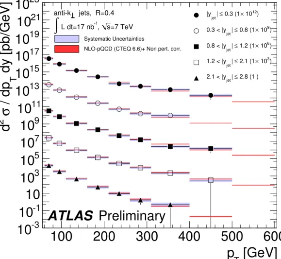
Figures 10 and 11 show the double-differential cross section as a function of jetpTin several different regions of rapidity. A selection of the same cross sections expressed as a function of rapidity in different pTranges are shown in Figs. 12 and 13. In Figs. 14 and 15 the ratio of the measurement to the theoretical prediction is shown for the double-differential distribution in jet pTforR=0.4 andR=0.6 respectively.
The data are again compared to NLO QCD predictions to which soft corrections have been applied. In all regions, the theory is consistent with the data.
In Figs. 16 and 17, the double-differential dijet cross section is shown as a function of the dijet mass, for different bins of the maximum rapidity of the two leading jets, |y|max=max(|y1|,|y2|). The cross section falls rapidly with mass, but extends up to masses of nearly 2 TeV. Figures 18 and 19 show the cross section as a function of the dijet angular variableχ for different ranges of the dijet massm12. The data are again compared to NLO perturbative QCD calculations corrected for non-perturbative effects.
The theory is consistent with the data.
In Figs. 20 and 21 the ratio of the measurement to the theoretical prediction is shown for the double- differential dijet cross sections forR=0.4 andR=0.6 respectively. The data are again compared to NLO QCD predictions to which soft corrections have been applied. In all regions, the theory is consistent with the data.
10-2
10-1
1 10 102
103
104
105
106
[GeV]
Truth pT
40 102 2×10²
resolution±Rapidity bias
-0.1 -0.05 0 0.05 0.1
ATLAS Preliminary
jets, R=0.6 anti-k
|<2.8 yj
|
10-3
10-2
10-1
1 10 102
103
104
105
106
[GeV]
Truth pT
40 102 2×10² resolution± fractional bias Tp
-0.4 -0.3 -0.2 -0.1 0 0.1 0.2 0.3
0.4 ATLAS Preliminary
jets, R=0.6 anti-k
|<2.8 yj
|
10-6
10-5
10-4
10-3
10-2
10-1
1 10 102
103
104
105
106
[GeV]
Truth m12
102
2× 10³ 2×10³
resolution± fractional bias 12m
-0.4 -0.3 -0.2 -0.1 0 0.1 0.2 0.3 0.4
ATLAS Preliminary
jets, R=0.6 anti-k
|<2.8 yj
|
10-4
10-3
10-2
10-1
1 10 102
103
104
[GeV]
Truth m12
102
4× 10³
resolution± fractional bias χ
-0.2 -0.15 -0.1 -0.05 0 0.05 0.1 0.15
0.2
ATLAS Preliminary
jets, R=0.6 anti-k
|<2.8 yj
|
Figure 3: The upper two plots show the absolute (fractional) resolution and bias in jety(pT) as a function of true pT. The bottom two plots show the fractional resolution and bias in dijet massm12and angular variable χ as a function of truem12. These are shown for all jets identified using the anti-k⊥ algorithm with R=0.6 in events passing the final kinematic selection, as predicted by Pythia 6. The error bar indicates the resolution and the central value indicates the bias. The contour plot indicates the underlying distribution, with the colour scale indicating the accepted MC cross section in pb.
100 200 300 400 500 600 dy [pb/GeV] T/dpσ2 d
10-3
10-1
10 103
105
107
109
1011
1013
1015
1017
1019
1021
ATLAS Preliminary
L dt=17 nb-1
∫
R = 0.4
0.91) Herwig(×
0.92)
× (
0
Pythia Perugia 0.69) Pythia MC09(×
=7 TeV) s (
12)
× 10 0.3 (
| ≤ 0 < |yjet
9)
× 10 0.8 (
| ≤ 0.3 < |yjet
6)
× 10 1.2 (
| ≤ 0.8 < |yjet
3)
× 10 2.1 (
| ≤ 1.2 < |yjet
1.0) 2.8 (×
| ≤ 2.1 < |yjet
1 2 3
≤ 0.3
jet| 0 < |y
1 2 3
≤ 0.8
jet| 0.3 < |y
1 2 3
≤ 1.2
jet| 0.8 < |y
1 2 3
≤ 2.1
jet| 1.2 < |y
200 400 600
1 2 3
≤ 2.8
jet| 2.1 < |y
Data / MC
[GeV]
pT
Figure 4: Inclusive jet double-differential cross section as a function of pT, for different bins of rapidity y. This is shown for jets identified using the anti-k⊥algorithm withR=0.4. The data are compared to leading-logarithmic parton-shower Monte Carlo simulations, normalised to the measured cross section by the factors shown in the legend. The band indicates the total systematic uncertainty on the data. The insets along the right-hand side show the ratio of the data to the various Monte Carlo simulations.
100 200 300 400 500 600 dy [pb/GeV] T/dpσ2 d
10-3
10-1
10 103
105
107
109
1011
1013
1015
1017
1019
1021
ATLAS Preliminary
L dt=17 nb-1
∫
R = 0.6
0.91) Herwig(×
0.92) (× Pythia Perugia0
0.69) Pythia MC09(×
=7 TeV) s (
12)
× 10 0.3 (
| ≤ 0 < |yjet
9)
× 10 0.8 (
| ≤ 0.3 < |yjet
6)
× 10 1.2 (
| ≤ 0.8 < |yjet
3)
× 10 2.1 (
| ≤ 1.2 < |yjet
1.0) 2.8 (×
| ≤ 2.1 < |yjet
1 2 3
≤ 0.3
jet| 0 < |y
1 2 3
≤ 0.8
jet| 0.3 < |y
1 2 3
≤ 1.2
jet| 0.8 < |y
1 2 3
≤ 2.1
jet| 1.2 < |y
200 400 600
1 2 3
≤ 2.8
jet| 2.1 < |y
Data / MC
[GeV]
pT
Figure 5: Inclusive jet double-differential cross section as a function of pT, for different bins of rapidity y. This is shown for jets identified using the anti-k⊥algorithm withR=0.6. The data are compared to leading-logarithmic parton-shower Monte Carlo simulations, normalised to the measured cross section by the factors shown in the legend. The band indicates the total systematic uncertainty on the data. The insets along the right-hand side show the ratio of the data to the various Monte Carlo simulations.
1 10
χ [pb/GeV] 12dMχ/dσ2 d10
-210
-11 10 10
210
310
410
510
610
7ATLAS Preliminary
=7 TeV) s
(
2)
× 10 520 GeV (
12≤ 340 < M
1)
× 10 800 GeV (
12≤ 520 < M
1.0)
× 1200 GeV (
12≤ 800 < M L dt=17 nb-1
∫
R = 0.4
0.91)
× Herwig(
0.92)
×
0( Pythia Perugia
0.69)
× Pythia MC09(
Figure 6: Dijet differential cross section as a function of angular variableχ in different regions of dijet massm12, for jets identified using the anti-k⊥algorithm withR=0.4. The data are compared to leading- logarithmic parton-shower Monte Carlo simulations, normalised to the measured cross section by the factors shown in the legend.
1 10
χ [pb/GeV] 12dMχ/dσ2 d10
-210
-11 10 10
210
310
410
510
610
7ATLAS Preliminary
=7 TeV) s
(
2)
× 10 520 GeV (
12≤ 340 < M
1)
× 10 800 GeV (
12≤ 520 < M
1.0)
× 1200 GeV (
12≤ 800 < M L dt=17 nb-1
∫
R = 0.6
0.91)
× Herwig(
0.92)
×
0( Pythia Perugia
0.69)
× Pythia MC09(
Figure 7: Dijet differential cross section as a function of angular variableχ in different regions of dijet massm12, for jets identified using the anti-k⊥algorithm withR=0.6. The data are compared to leading- logarithmic parton-shower Monte Carlo simulations, normalised to the measured cross section by the factors shown in the legend.
[GeV]
p
T100 200 300 400 500 600
[pb/GeV] T / dpσd
1 10 102
103
104
105
106
=7 TeV) s
-1 ( L dt=17 nb
∫
Systematic Uncertainties
NLO-pQCD (CTEQ 6.6)+ Non pert. corr.
ATLAS Preliminary
≤ 2.8
jet| jets, R=0.4, |y anti-k
[GeV]
pT
100 200 300 400 500 600
Data/Theory 0
0.5 1 1.5
2
Figure 8: Inclusive jet differential cross section as a function of jet pT integrated over the full region
|y|<2.8 for jets identified using the anti-k⊥ algorithm with R=0.4. The data are compared to NLO QCD calculations to which soft QCD corrections have been applied. The error bars indicate the statistical uncertainty on the measurement, and the grey shaded band indicates the quadratic sum of the systematic uncertainties, dominated by the jet energy scale uncertainty. There is an additional overall uncertainty of 11% due to the luminosity measurement that is not shown. The theory uncertainty shown in orange is the quadratic sum of uncertainties from the choice of renormalisation and factorisation scales, parton distribution functions,αs(MZ), and the modelling of soft QCD effects, as described in the text.
[GeV]
p
T100 200 300 400 500 600
[pb/GeV] T / dpσd
1 10 102
103
104
105
106
=7 TeV) s
-1 ( L dt=17 nb
∫
Systematic Uncertainties
NLO-pQCD (CTEQ 6.6)+ Non pert. corr.
ATLAS Preliminary
≤ 2.8
jet| jets, R=0.6, |y anti-k
[GeV]
pT
100 200 300 400 500 600
Data/Theory 0
0.5 1 1.5
2
Figure 9: Inclusive jet differential cross section as a function of jet pT integrated over the full region
|y|<2.8 for jets identified using the anti-k⊥ algorithm with R=0.6. The data are compared to NLO QCD calculations to which soft QCD corrections have been applied. The uncertainties on the data and theory are shown as described in Fig. 8.
[GeV]
p
T100 200 300 400 500 600 dy [pb/GeV]
T/ dp σ
2d
10
-310
-110 10
310
510
710
910
1110
1310
1510
1710
1910
2110
23Systematic Uncertainties
NLO-pQCD (CTEQ 6.6)+ Non pert. corr.
12)
× 10 0.3 (1
| ≤
|yjet
9)
× 10 0.8 (1
| ≤ 0.3 < |yjet
6)
× 10 1.2 (1
| ≤ 0.8 < |yjet
3)
× 10 2.1 (1
| ≤ 1.2 < |yjet
2.8 (1 )
| ≤ 2.1 < |yjet
ATLAS Preliminary
=7 TeV s
-1, L dt=17 nb
∫
jets, R=0.4 anti-k
Figure 10: Inclusive jet double-differential cross section as a function of jet pT in different regions of
|y|for jets identified using the anti-k⊥ algorithm with R=0.4. The data are compared to NLO QCD calculations to which soft QCD corrections have been applied. The uncertainties on the data and theory are shown as described in Fig. 8.
[GeV]
p
T100 200 300 400 500 600 dy [pb/GeV]
T/ dp σ
2d
10
-310
-110 10
310
510
710
910
1110
1310
1510
1710
1910
2110
23Systematic Uncertainties
NLO-pQCD (CTEQ 6.6)+ Non pert. corr.
12)
× 10 0.3 (1
| ≤
|yjet
9)
× 10 0.8 (1
| ≤ 0.3 < |yjet
6)
× 10 1.2 (1
| ≤ 0.8 < |yjet
3)
× 10 2.1 (1
| ≤ 1.2 < |yjet
2.8 (1 )
| ≤ 2.1 < |yjet
ATLAS Preliminary
=7 TeV s
-1, L dt=17 nb
∫
jets, R=0.6 anti-k
Figure 11: Inclusive jet double-differential cross section as a function of jet pT in different regions of
|y|for jets identified using the anti-k⊥ algorithm with R=0.6. The data are compared to NLO QCD calculations to which soft QCD corrections have been applied. The uncertainties on the data and theory are shown as described in Fig. 8.
jet
|
|y
0 0.5 1 1.5 2 2.5 3
dy [pb/GeV]
T/ dp σ
2d
10
-11 10 10
210
310
410
510
610
710
810
9Systematic Uncertainties
NLO pQCD (CTEQ 6.6)+ Non pert. corr.
< 80 GeV 60 GeV < pT
< 160 GeV 110 GeV < pT
< 260 GeV 210 GeV < pT
< 400 GeV 310 GeV < pT
ATLAS Preliminary
=7 TeV s
-1, L dt=17 nb
∫
jets, R=0.4 anti-k
Figure 12: Inclusive jet double-differential cross section as a function of jet |y|in different regions of pT for jets identified using the anti-k⊥ algorithm withR=0.4. The data are compared to NLO QCD calculations to which soft QCD corrections have been applied. The uncertainties on the data and theory are shown as described in Fig. 8.
jet
|
|y
0 0.5 1 1.5 2 2.5 3
dy [pb/GeV]
T/ dp σ
2d
10
-11 10 10
210
310
410
510
610
710
810
9Systematic Uncertainties
NLO pQCD (CTEQ 6.6)+ Non pert. corr.
< 80 GeV 60 GeV < pT
< 160 GeV 110 GeV < pT
< 260 GeV 210 GeV < pT
< 400 GeV 310 GeV < pT
ATLAS Preliminary
=7 TeV s
-1, L dt=17 nb
∫
jets, R=0.6 anti-k
Figure 13: Inclusive jet double-differential cross section as a function of jet |y|in different regions of pT for jets identified using the anti-k⊥ algorithm withR=0.6. The data are compared to NLO QCD calculations to which soft QCD corrections have been applied. The uncertainties on the data and theory are shown as described in Fig. 8.