ATLAS NOTE ATLAS-CONF-2010-082

(1)

ATLAS-CONF-2010-082 11October2010

ATLAS NOTE

ATLAS-CONF-2010-082

August 20, 2010

Angular correlations between charged particles from proton-proton collisions at √

s = 900 GeV and √

s = 7 TeV measured with ATLAS detector

The ATLAS Collaboration

Abstract

This note describes a study of angular correlations between charged primary particles stemming from proton-proton collisions at the Large Hadron Collider. Two observables are defined based on∆φ, the angle in the transverse plane between the particle with the highest transverse momentum and any other particle in the collision. The shapes of the observables have a very small systematic uncertainty and are different for√

s= 900 GeV and 7 TeV. The distributions observed in data are compared to different tunes of the PYTHIAevent generator.

(2)

1 Introduction

The non-perturbative nature of QCD makes it necessary to develop heuristic descriptions of processes that cannot be approximated otherwise. Typically, these are “soft” processes such as the development of showers in jets and the underlying event (usually defined as multiple parton interaction (MPI) beam remnants and initial state radiation). Packages such as Pythia [1] or Herwig [2], that describe these processes need to be tuned using experimental input [3, 4]. Charged particle multiplicities as a function of pseudorapidity (η) and mean transverse momentum of particles as a function of their multiplicity are commonly used as input variables to these tunes [5]. Consequently, tunes derived from comparisons to these observables should describe these variables well. Due to the complexity of the modelling required, these variables cannot be assumed to describe the entirety of the processes and constrain the parameteri- sation of the models sufficiently. Identifying new experimental observables can provide further insights into the non-perturbative processes themselves. They provide further inputs to the tuning process, especially if they allow us to probe areas where the behavior of the various tunes differ. Finally, these variables can be designed to minimize or avoid the influence of the systematic effects that dominate the measurements of observables like number of particles as a function of pseudorapidity, where the absolute tracking efficiency (and it’s associated error) is a crucial input.

The distribution of the angles in the transverse plane (∆φ) between the leading particle in a minimum bias event and all other particles has been studied before [6, 7, 8, 9]. Intervals of∆φ are labeled “away”,

“transverse” and “toward” regions, defined relative to the position of the leading particle. The toward and away regions are supposed to contain most of the jets recoiling against or located around the leading particle. The transverse region should be mostly devoid of these and characterize the underlying event.

The number of particles in the “transverse region” has been used to study the underlying event – usually as a function of the leading particle’s transverse momentum. The transverse region is assumed to be dominated by the underlying event, and not by the emerging very soft jets from soft QCD 2→2 processes.

However, the study presented in this note shows that different models of soft QCD processes (MPI but also initial and final state radiation, treatment of beam remnants and color reconnections) provide significantly different predictions of the width and height of the toward and away-side peaks, making the characteristics of these peaks an interesting object of study. Our study is complementary to those aimed at the transverse region: we will study explicitly the toward and away-side peaks. In the following we will see how a special definition of the observables extracts just these and is able to reduce the impact of systematic uncertainties in the tracking efficiency.

1.1 Definition of observables

In this note the charged particle with highest transverse momentum (pT) in a proton-proton collision is called theleading particleand all other particles are callednon-leading particles. The azimuthal angular difference,∆φ, is defined as the unsigned angle in the transverse (x-y) plane between the leading particle and any non-leading particle. The following two distributions derived from∆φ are studied.

1.1.1 ∆φ crest shape

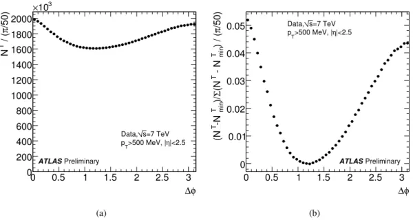
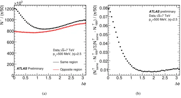
The raw∆φdistribution is obtained by histograming∆φfor all non-leading particles in an event. The resulting distribution presents two characteristic enhancements at zero andπ, the so-called crest, sitting on top of a large “pedestal” of particles, as can be seen in Fig. 1a. The number of entries in a given∆φinter- val is labeledN^T. The minimum of this distribution (N_min^T ) is determined by a second order polynomial fit and subtracted from the value in each bin. The resulting distribution is normalised to unit area, thus keep- ing only the shape of the crest of the raw distribution, as shown in Fig. 1b. Since the∆φ range is divided

(3)

φ

∆

0 0.5 1 1.5 2 2.5 3

/50)π / ( T N

0 200 400 600 800 1000 1200 1400 1600 1800 2000

103

×

|<2.5 η

>500 MeV, | pT

=7 TeV s Data,

Preliminary ATLAS

(a)

φ

∆

0 0.5 1 1.5 2 2.5 3

/50)π) / ( min T - N T (NΣ)/ min T -N T (N

0 0.01 0.02 0.03 0.04

0.05 >500 MeV, |η|<2.5 pT

=7 TeV s Data,

(b)

Figure 1:(a)∆φdistribution of all selected tracks in the 7 TeV data.(b)∆φdistribution of selected tracks after the subtraction of the minimum and normalised to unit area. For these plots no corrections to the reconstructed distributions are applied. The errors are statistical only and are smaller than the markers.

into 50 intervals, the result of these manipulations is expressed as(N^T−N_min^T )/∑(N^T−N_min^T )/(π/50), where the summation goes over all 50 intervals.

1.1.2 ∆φ “same minus opposite”

To create the∆φ “same minus opposite” observable, each event is divided into twoη regions according to theη of the leading particle. ∆φ is histogramed separately for particles with η of the same sign as the leading particle and for particles withη of the opposite sign. This results in the “same region” and

“opposite region”∆φ distributions (Fig. 2a), respectively, withN_same^T andN_opp^T entries in a∆φ interval.

The “opposite region” distribution is subtracted from the “same region” distribution and the resulting distribution is normalised to unit area (Fig. 2b). The resulting value in each of the 50∆φintervals is thus expressed as(N_same^T −N_opp^T )/∑(N_same^T −N_opp^T )/(π/50). Note that the regions defined are not the same as the forward and backward halves of the detector, but an almost even mix of those, since in roughly half of the events the leading track is in the positive η region and in the other half of the events it is in the negativeη region. This observable incorporates some of the pseudorapidity correlation between particles while retaining the desired robustness and low systematic uncertainties.

The aim of this measurement is to reconstruct the∆φ distributions of charged primary particles created in a proton-proton collision (data corrected to the particle level to correct for detector effects) within the following phase space:

• pT>500 MeV,

• three pseudorapidity ranges: |η|<2.5,|η|<2.0,|η|<1.0,

• two or more charged primary particles within above kinematic range.

(4)

φ

∆

0 0.5 1 1.5 2 2.5 3

/50)π / ( T N

0 200 400 600 800 1000 1200

103

×

Same region Opposite region

|<2.5 η

>500 MeV, | pT

=7 TeV s Data,

(a)

φ

∆

0 0.5 1 1.5 2 2.5 3

/50)π) / ( opp T - N same T (NΣ)/ opp T - N same T (N 0.01

0.02 0.03 0.04 0.05 0.06 0.07 0.08

|<2.5 η

>500 MeV, | pT

=7 TeV s Data,

preliminary ATLAS

(b)

Figure 2: (a)reconstructed “same” region (black) and “opposite” region (red)∆φ distributions in the 7 TeV data. (b)the normalised “same minus opposite”∆φ distribution. No corrections are applied to the reconstructed distributions. The errors are statistical only and are smaller than the markers.

2 The ATLAS detector

The ATLAS detector [10] covers a large solid angle around the collision point with layers of tracking detectors, calorimeters and muon chambers. It has been designed to study a wide range of physics topics at LHC energies. For the measurements presented in this note, the trigger system and the tracking devices were of particular importance.

The ATLAS inner detector has full coverage inφ and covers the pseudorapidity range|η|<2.5. It consists of a silicon pixel detector (Pixel), a silicon strip detector (SCT) and a transition radiation tracker (TRT). These detectors cover a sensitive radial distance from the interaction point of 50.5mm - 150 mm, 299 - 560 mm and 563 - 1066 mm, respectively, and are immersed in a 2 Tesla axial magnetic field.

The inner detector barrel (end-cap) parts consist of 3 (2×3) Pixel layers, 4 (2×9) layers of double-sided silicon strip modules, and 73 (2×160) layers of TRT straws. These detectors have position resolutions of typically 10, 17 and 130µm for the r-φcoordinate and, in case of the Pixel and SCT, 115 and 580µm for the r-z coordinate. A track traversing the barrel would typically have 11 silicon hits (3 pixel clusters, and 8 strip clusters), and more than 30 straw hits.

The ATLAS detector has a three-level trigger system: Level 1 (L1), Level 2 (L2) and the Event Filter (EF). For this measurement, the trigger relies on the Beam Pickup Timing devices (BPTX) and the Minimum-Bias Trigger Scintillators (MBTS). The BPTX are composed of electrostatic beam pick-ups attached to the beam pipe±175 m from the center of the ATLAS detector. The MBTS are mounted at each end of the detector in front of the liquid-argon endcap-calorimeter cryostats at z =±3.56 m and are segmented into eight sectors in azimuth and two rings in pseudorapidity (2.09<|η|<2.82 and 2.82<|η|<3.84). Data were taken for this analysis using the L1 MBTS trigger, formed from L1 BPTX and MBTS trigger signals. The L1 MBTS trigger was configured to require one hit above threshold from either side of the detector. For events with at least two charged particles within the phase space of this analysis the trigger efficiency is above 99.9%.

The coordinate system is defined in the following way: thez-axis is along the beam, they-axis points upwards and the x-axis points towards the center of the LHC. Its origin is at the center of the ATLAS

(5)

detector.

3 Datasets and selection criteria

The definition of a primary particle, the dataset used for this measurement, the event selection and the track selection follow those described in [11] and are summarised below. The only difference is in the chosen phase space: the transverse momentum range for this measurement is chosen to bep_T>500 MeV rather than 100 MeV. The reason for this choice is to avoid the region where the tracking efficiency varies greatly and in this way decrease the systematic uncertainty. Measurements in pseudorapidity ranges

|η|<2.0 and |η|<1.0 are also performed for comparison with other measurements and to provide additional information for comparison with Monte Carlo models.

The 900 GeV data were taken in December 2009 and correspond to an integrated luminosity of about 7 µb⁻¹. The 7 TeV data were taken during the first LHC runs at that energy in March and April 2010 and correspond to an integrated luminosity of about 190µb⁻¹.

Primary charged particles are defined as charged particles with a mean lifetime τ >0.3·10⁻¹⁰s directly produced in proton-proton interactions or from subsequent decays of particles with a shorter lifetime.

Selected events are required to

• have passed the Level 1 Minimum Bias Trigger Scintillator (MBTS) single-arm trigger,

• have a reconstructed primary vertex,

• not have a second reconstructed primary vertex with four or more tracks in the same bunch crossing (to remove pile-up),

• have at least two tracks that pass the selection described below.

The first three requirements have a very high efficiency and a negligible effect on the observed distributions, whereas the requirement of at least two selected tracks does have some impact.

The track selection consists of the following requirements:

• pT>500 MeV,

• |η|<2.5 (varied to 2.0 and 1.0),

• at least 1 hit in the Pixel detector,

• at least 6 hits in the SCT,

• transverse and longitudinal impact parameters with respect to the primary vertex|d₀^PV|<1.5 mm and|z^PV₀ sinθ^PV|<1.5 mm, respectively.

For the validation of the measurement method, events generated by Pythia event generator were used, followed by a full detector simulation and reconstruction. For√s=900 GeV the amount of MC used is about 1.5 times the data sample size and for√

s=7 TeV it is about two thirds the data sample size. Non- diffractive, single-diffractive and double-diffractive events were used. It was checked, that the impact of the diffractive components is small and does not affect the conclusions. As a cross-check, the analysis was repeated with events generated by Phojet generator, again resulting in the same conclusions as using the default MC sample.

(6)

0 0.5 1 1.5 2 2.5 3 /50)π)/(minT-NT(NΣ)/minT-NT(N

0 0.01 0.02 0.03 0.04 0.05 0.06 0.07

0 0.5 1 1.5 2 2.5 3

/50)π)/(minT-NT(NΣ)/minT-NT(N

0 0.01 0.02 0.03 0.04 0.05 0.06

0.07 ATLAS Preliminary

MC generated MC reconstructed = 7 TeV s MC,

> 500 MeV pT

| < 2.5 η

|

φ

∆

0 0.5 1 1.5 2 2.5 3

Difference

-0.002 -0.001 0 0.001 0.002

(a)

0 0.5 1 1.5 2 2.5 3

/50)π)/(oppT-Nsame

T (NΣ)/oppT-Nsame

T (N

0 0.02 0.04 0.06 0.08 0.1 0.12

0 0.5 1 1.5 2 2.5 3

/50)π)/(oppT-Nsame

T (NΣ)/oppT-Nsame

T (N

0 0.02 0.04 0.06 0.08 0.1 0.12

ATLAS Preliminary

MC generated MC reconstructed = 7 TeV s MC,

> 500 MeV pT

| < 2.5 η

|

φ

∆

0 0.5 1 1.5 2 2.5 3

Difference

-0.002 -0.001 0 0.001 0.002

(b)

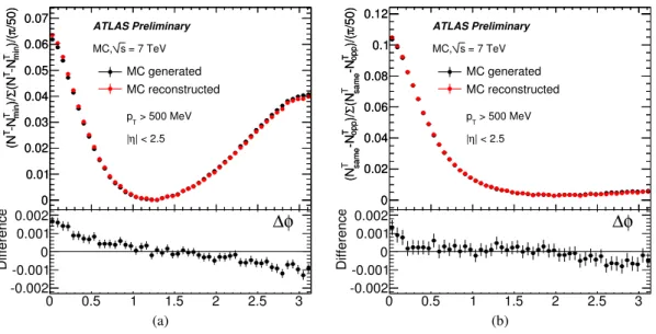
Figure 3: ∆φ crest shape (a)and “same minus opposite”(b)in 7 TeV Monte Carlo events. The black markers show the generated distributions and the red markers the reconstructed ones without applying any correction. One can notice a reasonably good agreement between generated and reconstructed distributions, demonstrating the robustness of the constructed observables. The errors are statistical only.

4 Reconstructed ∆φ distribution and the correction procedure

Due to experimental effects the measured∆φ distribution of selected tracks differs from the∆φ distribution of charged primary particles. These effects were studied in detail with Monte Carlo simulation.

Several comparisons between data and MC were made to make sure that the simulation describes the data well and to find possible differences. In this section these studies are summarised, and the correction procedure applied to compensate for the experimental effects is described.

4.1 Uncorrected∆φ distributions

Fig. 1 shows the “raw”∆φdistributions of all selected tracks before the subtraction of the minimum and normalisation (a) and the uncorrected∆φ crest shape after the minimum subtraction and normalisation to unit area (b). In Fig. 2a the∆φ distributions are shown separately for “same” region and “opposite”

region. Fig. 2b shows the uncorrected normalised “same minus opposite”∆φdistribution. All these plots are for for 7 TeV data and no corrections are applied to these reconstructed distributions.

Using Monte Carlo simulation it was verified that the reconstructed∆φ crest shape and “same minus opposite” distribution reproduce reasonably well the distributions obtained from the generated particles, even without applying any corrections. The agreement is illustrated in Fig. 3 and demonstrates the robustness of the constructed observables. However, one can see that the ∆φ distributions are slightly modified by the detector effects. Applying the correction procedure described in Section 4.6, the observed disagreement between the generated and reconstructed distributions on Monte Carlo is to a large extent recovered.

(7)

4.2 Effects of event selection inefficiency

A small fraction of events is lost due to event selection, mostly due to the requirement of at least two selected tracks. These are mostly low multiplicity events with a small contribution to the∆φdistributions.

To quantify the effect, the∆φdistribution of generated particles in events which pass the event selection was compared to the∆φ distribution of generated particles in all Monte Carlo events. The difference between the two was found to be a few tenths of a percent and is accounted for as a systematic uncertainty.

Here and in the following the relative uncertainties are stated in percentage of the measured quantities in the first bin, where the absolute uncertainties are the biggest.

4.3 Effect of tracking inefficiency

Effects of tracking inefficiency were studied thoroughly and are described here. Tracking inefficiency affects the∆φ distribution in two ways: through the loss of the leading track and through the loss of the non-leading tracks. For the effect of losing the non-leading tracks the non-homogeneity of the tracking efficiency is more important than its average value. On the other hand, the effect of losing the leading track, to a largest extent, depends on the absolute value of the efficiency.

The effect of inhomogeneities in theφ dependence of the tracking efficiency cancels out to a great extent. This was derived analytically and further studied by randomly throwing away some generated particles in accordance with aφ-dependent tracking efficiency extracted from data. The study confirmed that the effect on the∆φdistribution is very small and is treated as a source of the systematic uncertainty.

The “same minus opposite” distribution could be affected by different tracking efficiencies of the two halves of the detector with positive and negativeηvalues. This effect also cancels in the leading order.

The difference in the tracking efficiency for both detector halves was estimated in data from the number of reconstructed tracks in each half of the detector. The difference is about 0.15%. It was propagated to extract the effect on the∆φ distribution and it was found to be negligible.

Using Monte Carlo simulated events it was found that the tracking efficiency dependence onpT and η affects the∆φ distributions significantly. This is due to the fact that p_T andη distributions of tracks are not equal in all∆φ bins. The meanpT and meanηas a function of∆φ were studied in data and MC.

Their variation in MC is larger than in data. This means that the observed ∆φ distortions observed on MC are larger than those present in the data. The effect is corrected for as described in Section 4.6.

A particular consideration was given to events where the leading particle is not reconstructed. In such events the observed leading track most often corresponds to the particle with the second highestpT, which results in a slightly different∆φ distribution. The difference in∆φ shape is verified to be small and is corrected for by a data driven method as described in Section 4.6.

4.4 Effect of tracking resolution

Using Monte Carlo simulation we find that in about 4% of events (for the|η|<2.5 range) the leading particle is reconstructed, but due to the resolution another track has a higher pT. In about 72% of such events the leading track is matched to the second-leading particle. Since the leading particle in these events is reconstructed, the ∆φ distributions are different from those where the leading particle is not reconstructed. Therefore one cannot correct for this effect in the same way as the effect of the lost leading particle is corrected for. A systematic uncertainty is extracted from Monte Carlo to cover this effect and is small, 0.1%-0.2%.

Effects ofpT andη resolution at the edge of the defined phase space (pT >500 MeV,|η|<2.5) are also included in the systematic uncertainty.

(8)

φ

0 0.5 1 1.5 2 2.5 ∆3

/50)π / ( T N

0 500 1000 1500 2000 2500

103

×

Corrected others, corrected lead Corrected others

Corrected others, -20% lead tracks Corrected others, -40% lead tracks Corrected others, -60% lead tracks Corrected others, -80% lead tracks Corrected others, -100% lead tracks

(a)

Percentage of true leading tracks

0 20 40 60 80 100

Number of tracks in 7th bin

2000 2050 2100 2150 2200 2250

103

×

(b)

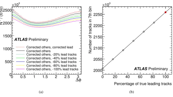
Figure 4: To simulate the effect of the reconstruction inefficiency of the leading particle, the leading track is disregarded in a fraction of events. The resulting ∆φ distributions are shown in plot (a). To illustrate the correction for the lost leading particle, in plot(b)the values from one of the bins in these distributions are plotted against the fraction of events where the leading track was not disregarded. The red full circle shows the extrapolated value, used as the final result. The extrapolated value is obtained in all∆φ bins and the resulting distribution is shown in plot (a) with the dashed red line, which lies above the other curves.

4.5 Effect of reconstructed non-primary particles and fake tracks

A small fraction of tracks (about 2%) is due to non-primary particles and tracks not stemming from proton-proton collision, and can be divided into two components: tracks correlated with the leading track and tracks uncorrelated with the leading track. The uncorrelated tracks are characterised by a flat

∆φ distribution and cancel in the subtraction described in Section 1.1. Such tracks would stem from detector noise, beam background, cosmic muons or an additional proton-proton collision in a triggered collision event. The correlated non-primary tracks exhibit a∆φ distribution similar to the primary tracks with slightly enhanced values at low ∆φ. These tracks typically originate from interaction with the detector material and decays of long-lived particles.

The fraction of non-primary tracks depends onpTandηof the measured track and is corrected for as described in Section 4.6. Since the correction cannot account for angular correlation between the leading and the non-leading track, the small enhancement at low∆φ values is not remedied completely and is taken into account as a part of the systematic uncertainty.

4.6 Corrections and residual bias

To correct for the loss of the non-leading tracks due to tracking inefficiency and for the contamination from non-primary tracks,∆φhistograms are filled with a weight which depends on p_T andηof the non- leading track. The weight is calculated as w= (1−bkg)/ε, wherebkgandε are pT andη dependent fraction of non-primary tracks and efficiency, respectively, extracted from Monte Carlo simulation.

To correct for the loss of the leading track one needs to know the fraction of events where the leading track is lost, and the∆φ distribution in these events. The fraction of events where the leading track is lost is extracted by averaging the p_T-η dependent MC efficiency over thep_T-ηdistribution of the data.

(9)

For |η|<2.5 it amounts to approximately 19%. The shape of the∆φ distribution in these events is fully extracted from the data by ignoring the leading track and measuring∆φagainst the second leading track. The correction for the loss of the leading track is extracted in the following way. In data the leading track is ignored and∆φ is measured against the second leading track in 0%, 20%, 40%, 60%, 80% and 100% of randomly selected events. This procedure results in six “raw”∆φdistributions, shown in Fig. 4a. In Fig. 4b, the number of reconstructed (non-leading) tracks in a single delta-phi bin is plotted against the percentage of events in which the true leading track was not removed, demonstrating a linear dependence between these two quantities. For each bin of the∆φdistribution the six points are fitted with a straight line and the value extrapolated to the 100% leading track efficiency is taken as the corrected value. By generating MC experiments in which generated particles were randomly excluded to simulate the tracking efficiency, the method was proved to work, however with a small positive bias in the lowest

∆φ region, which is accounted for as a part of the systematic error.

After applying these two corrections we observe on Monte Carlo a small remaining difference between the corrected∆φ distribution and the∆φ distribution of the generated particles. Studies showed that this difference arises partially due to secondary particles correlated to the leading track and partially due to the bias in the correction for the lost leading track as described above.

5 Estimate of systematic uncertainties

In this section systematic uncertainties are summarised and quantified. The relative systematic uncertainties are quoted for the first few bins of the∆φdistributions, where the systematic effects are largest.

• Using Monte Carlo simulation it was checked that event selection inefficiency has a small effect.

To study the effect in data, the requirement of at least two reconstructed tracks in an event was increased to three and four. Since the effect of this variation in data is different from the one in Monte Carlo, we extract a very conservative systematic uncertainty due to event selection inefficiency from data. We compare the ∆φ distributions in events with at least three selected tracks with the default result and take the difference as a systematic uncertainty. Its size is about 1% in the 7 TeV sample and about 3% in the 900 GeV sample.

• The small residual bias in the first four bins of the ∆φ distribution is covered by applying an additional 2% systematic uncertainty in these bins.

• An estimate of the systematic uncertainty due to tracking resolution effects in the vicinity of the boundaries of the kinematic phase space (p_T >500 MeV,|η|<2.5) was obtained from data by varying thepT andηcuts within their resolutions and repeating the analysis. The difference from the default result was added bin-by-bin as the systematic uncertainty. Its size is 1%-2% for the pT

variation and 0.2%-0.5% for theηvariation.

• The tracking resolution effect on selecting a false leading particle (the leading particle is reconstructed, but another track has a higher p_T) was estimated from Monte Carlo. It results in a 0.1%-0.2% systematic uncertainty and is evaluated bin-by-bin.

• Uncertainty on the fraction of events where the leading particle is not reconstructed, which is (19±3)% for|η|<2.5. The final distributions are remade with the leading track’s inefficiency changed to 22% and 16% (and in the other twoη ranges accordingly). The resulting differences from the default result are taken as the systematic uncertainty bin-by-bin in the distributions of the observables. They are of the order of a few tenths of a percent.

(10)

• Uncertainty on the tracking efficiencies used to correct for the missing non-leading tracks. The average tracking inefficiency is about (20±3)%. (Since the non-leading tracks have a softer p_T spectrum than the leading tracks, this inefficiency is slightly higher than the one in the previous point.) The systematic uncertainty from this source is estimated by comparing the non-corrected

∆φ distribution with the one corrected with the weight of (1−bkg)/ε and taking 15% of the difference as the systematic uncertainty (since 3/20=0.15). The resulting uncertainty is smaller than 0.2%.

• The tracking efficiency dependence on the detector angleφ results in an average absolute uncertainty of 6×10⁻⁵. This value is assigned as the absolute systematic uncertainty from this source in all bins. In the lowest∆φ bins this translates into a 0.1%-0.2% relative systematic uncertainty.

• To account for possible differences between data and Monte Carlo in the effect of correlated sec- ondaries, the measurement is redone with a variedd^PV₀ cut which determines the fraction of this component the most. The difference from the default result is taken as a systematic uncertainty and amounts on average to 9×10⁻⁵; this value is added in quadrature to the uncertainty of each bin. For the lowest∆φ bins the relative uncertainty is 0.1%-0.3%.

• The tracking efficiency difference between the two halves of the detector was found to have a negligible effect.

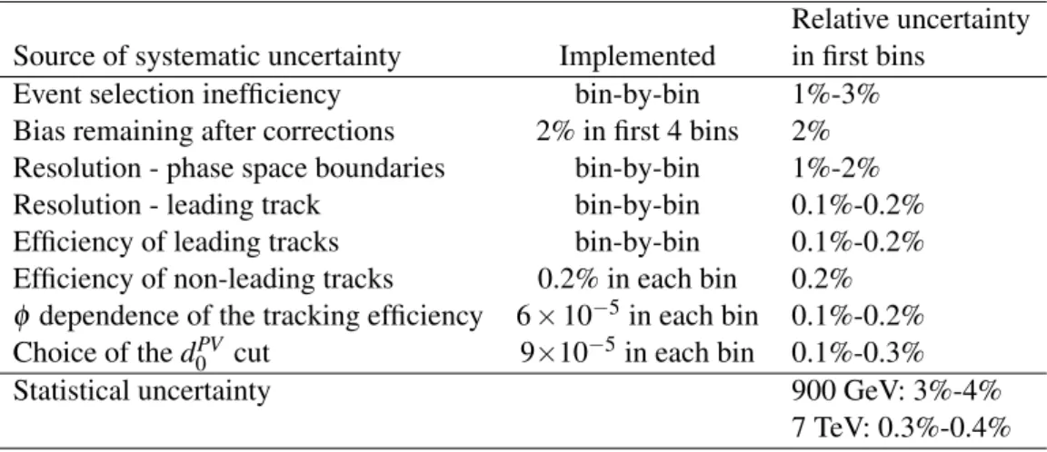
The summary of the systematic uncertainties is given in Table 1. The total uncertainty is obtained by adding in quadrature the systematic uncertainties to the statistical one.

Table 1: Systematic uncertainties, summary table

Relative uncertainty Source of systematic uncertainty Implemented in first bins

Event selection inefficiency bin-by-bin 1%-3%

Bias remaining after corrections 2% in first 4 bins 2%

Resolution - phase space boundaries bin-by-bin 1%-2%

Resolution - leading track bin-by-bin 0.1%-0.2%

Efficiency of leading tracks bin-by-bin 0.1%-0.2%

Efficiency of non-leading tracks 0.2% in each bin 0.2%

φ dependence of the tracking efficiency 6×10⁻⁵in each bin 0.1%-0.2%

Choice of thed₀^PV cut 9×10⁻⁵in each bin 0.1%-0.3%

Statistical uncertainty 900 GeV: 3%-4%

7 TeV: 0.3%-0.4%

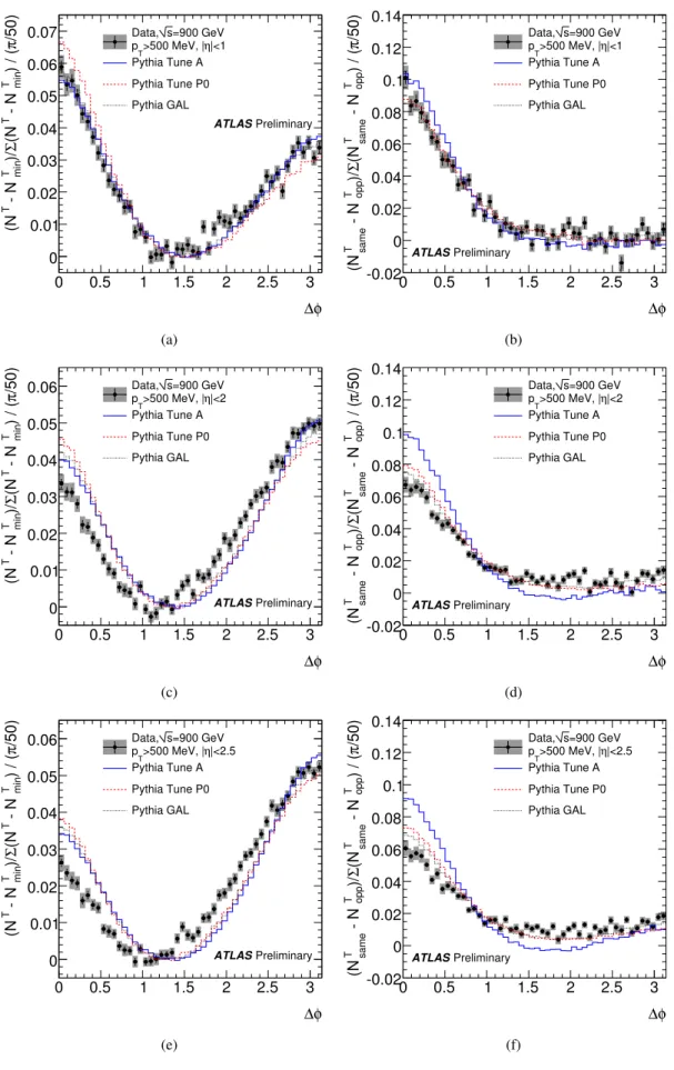
6 Results

The results of this measurement are∆φ crest shape and “same minus opposite” distributions shown in Figures 5 and 6 for √

s=900 GeV and √

s=7 TeV, respectively. The comparison between the two energies shows that the shapes are energy dependent. The distributions are compared to three Pythia tunes: tune A [12], tune Perugia0 [5] and GAL [13]. Tune A is a representative of the family of tunes that use virtuality-ordered showers. Perugia0 is a representative of the family of tunes that usepT-ordered showers. GAL is a tune using the Generalized Area Law of color reconnections and is a representative of the family of tunes that use different color reconnection models. Comparisons to more Pythia tunes are added in the Appendix.

(11)

We observe the best agreement between data and theory curves in the region|η|<1.0. This is not surprising, as a lot of tunes use TeVatron data from CDF as input, which is limited to this range. The agreement is not perfect, however, especially in the crest shape at 7 TeV where the recoil peak shape is not well-modelled.

As the η range is extended, two phenomena are observed. First, the theory curves, especially at 900 GeV, drift apart, exhibiting very different behaviour. This means that our measurement has a real possibility to discriminate between tunes. Second, even though the theory curves cover a large range of possible behaviours, none of them matches the data well. The further the η range is extended, the worse the match between data and theory. It appears that the extendedη reach of the ATLAS detector relative to previous tuning inputs is an asset for tuning work. With this, we come a full circle back to our stated goal to provide measurements of new observables that give tuners interesting handles on soft QCD processes. Our observables probe a range where the behaviour of current tunes is very different and shows that the further tuning is necessary to reproduce the measured data distributions.

7 Conclusion

Angular correlations between charged particles generated in proton-proton collisions were studied. The variable ∆φ is defined as the angle in the transverse plane between the leading particle and any other particle in the collision. The ∆φ crest shape and the “same minus opposite” distributions have proved to be robust observables with small systematic uncertainties. They were measured for particles with pT >500 MeV and in three different pseudorapidity ranges: |η|<2.5, 2.0, 1.0. Events containing at least two such particles were used. The shapes are found to be different in collisions with√

s=900 GeV and√

s=7 TeV. They are compared to a number of MC tunes and provide useful information for further improvements of the tunes.

References

[1] T. Sjostrand, S. Mrenna, and P. Z. Skands,PYTHIA 6.4 Physics and Manual, JHEP0605(2006) 026. [arXiv:hep-ph/0603175].

[2] G. Corcella, I. Knowles, G. Marchesini, S. Moretti, K. Odagiri, P. Richardson, M. Seymour, and B. Webber,HERWIG 6.5: an event generator for Hadron Emission Reactions With Interfering Gluons (including supersymmetric processes), JHEP0101(2001) 010. [hep-ph/0011363];

[hep-ph/0210213].

[3] R. K. Ellis, W. J. Stirling, and B. R. Webber,QCD and collider physics, Camb. Monogr. Part.

Phys. Nucl. Phys. Cosmol.8(1996) 1–435.

[4] Particle Data Group Collaboration, C. Amsler et al.,Review of particle physics, Phys. Lett.B667 (2008) 1.

[5] P. Z. Skands,The Perugia Tunes, . arXiv:0905.3418 [hep-ph].

[6] CDF Collaboration,Underlying event in hard interactions at the Fermilab Tevatron p-p collider, Phys. Rev. D70(2004) 072002.

[7] CDF Collaboration, T. Aaltonen et al.,Studying the underlying event in Drell-Yan and high transverse momentum jet production at the Tevatron, Phys. Rev. D82(2010) 034001.

(12)

φ

∆

0 0.5 1 1.5 2 2.5 3

/50)π) / ( min T - N T (NΣ)/ min T - N T (N

0 0.01 0.02 0.03 0.04 0.05 0.06 0.07

|<1 η

>500 MeV, | pT

=900 GeV s Data, Pythia Tune A Pythia Tune P0 Pythia GAL

(a)

φ

∆

0 0.5 1 1.5 2 2.5 3

/50)π) / ( opp T - N same T (NΣ)/ opp T - N same T (N -0.02

0 0.02 0.04 0.06 0.08 0.1 0.12 0.14

|<1 η

>500 MeV, | pT

(b)

φ

∆

0 0.5 1 1.5 2 2.5 3

0 0.01 0.02 0.03 0.04 0.05

0.06 >500 MeV, |η|<2 pT

(c)

φ

∆

0 0.5 1 1.5 2 2.5 3

/50)π) / ( opp T - N same T (NΣ)/ opp T - N same T (N

-0.02 0 0.02 0.04 0.06 0.08 0.1 0.12 0.14

|<2 η

>500 MeV, | pT

(d)

φ

∆

0 0.5 1 1.5 2 2.5 3

0 0.01 0.02 0.03 0.04 0.05

0.06 >500 MeV, |η|<2.5 pT

(e)

φ

∆

0 0.5 1 1.5 2 2.5 3

0 0.02 0.04 0.06 0.08 0.1 0.12 0.14

|<2.5 η

>500 MeV, | pT

(f)

Figure 5: The ∆φ crest shapes (a,c,e) and the “same minus opposite” distributions (b,d,f) at √ s = 900 GeV for three different pseudorapidity regions: |η|<1.0 (a,b), |η|<2.0 (c,d), |η|<2.5 (e,f).

The data (black dots) is compared to the predictions of three different Pythia tunes [12, 5, 13] (see text for more details). The vertical bars on the data points represent the statistical uncertainty while the

11

(13)

φ

∆

0 0.5 1 1.5 2 2.5 3

0 0.02 0.04 0.06 0.08 0.1

|<1 η

>500 MeV, | pT

=7 TeV s Data, Pythia Tune A Pythia Tune P0 Pythia GAL

(a)

φ

∆

0 0.5 1 1.5 2 2.5 3

-0.02 0 0.02 0.04 0.06 0.08 0.1 0.12 0.14

|<1 η

>500 MeV, | pT

(b)

φ

∆

0 0.5 1 1.5 2 2.5 3

0 0.01 0.02 0.03 0.04 0.05 0.06 0.07 0.08

|<2 η

>500 MeV, | pT

(c)

φ

∆

0 0.5 1 1.5 2 2.5 3

-0.02 0 0.02 0.04 0.06 0.08 0.1 0.12 0.14

|<2 η

>500 MeV, | pT

(d)

φ

∆

0 0.5 1 1.5 2 2.5 3

0 0.01 0.02 0.03 0.04 0.05

0.06 >500 MeV, |η|<2.5 pT

(e)

φ

∆

0 0.5 1 1.5 2 2.5 3

0 0.02 0.04 0.06 0.08 0.1 0.12 0.14

|<2.5 η

>500 MeV, | pT

(f)

√

(14)

[8] D0 Collaboration,Study ofφ andη correlations in minimum bias events with the D0 detector at the Fermilab Tevatron Collider, D0 Note 6054-CONF (2010) .

[9] ATLAS Collaboration, G. Aad et al.,Track-based underlying event measurements in pp collisions at√

s=900GeV and 7 TeV with the ATLAS Detector at the LHC, ATLAS-CONF-2010-029 (2010) .

[10] ATLAS Collaboration, G. Aad et al.,The ATLAS Experiment at the CERN Large Hadron Collider, JINST3(2008) S08003.

[11] ATLAS Collaboration,Charged particle multiplicities in pp interactions with a lowered p_T threshold at√

s = 0.9 and 7 TeV measured with the ATLAS detector at the LHC, ATLAS-CONF-2010-046 (2010) .

[12] R. D. Field,The underlying event in hard scattering processes,In the Proceedings of APS / DPF / DPB Summer Study on the Future of Particle Physics (Snowmass 2001), Snowmass, Colorado, 30 Jun - 21 Jul 2001, pp P501. [arXiv:hep-ph/0201192].

[13] J. Rathsman,A generalised area law for hadronic string reinteractions, Phys. Lett. B452(1999) 364. [arXiv:hep-ph/9812423],http://www.isv.uu.se/thep/MC/scigal/,

http://www3.tsl.uu.se/ rathsman/gal/.

[14] R. Field,Min-Bias and the Underlying Event at the Tevatron and the LHC, A talk presented at the Fermilab ME/MC Tuning Workshop, Fermilab, Oct 2002 .

[15] A. Buckley, H. Hoeth, H. Lacker, H. Schulz, and J. E. von Seggern,Systematic event generator tuning for the LHC, Eur. Phys. J. C65(2010) 331. [arXiv:0907.2973 [hep-ph]].

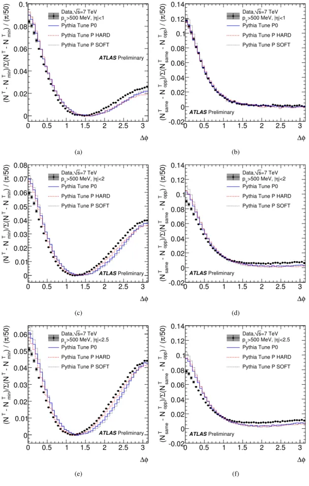
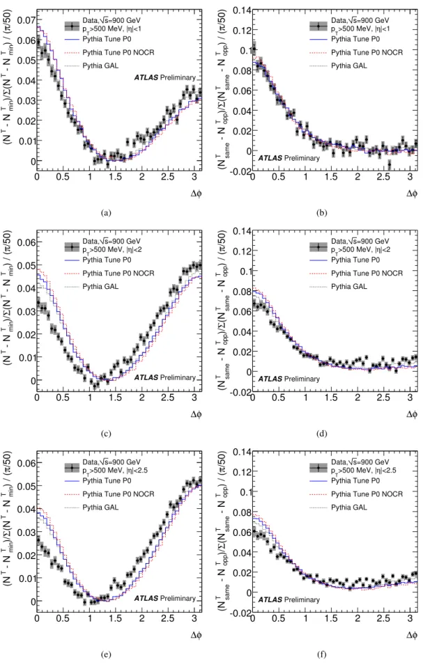
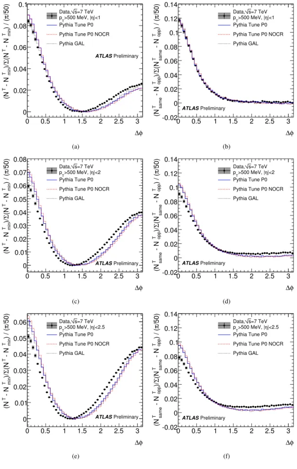
8 Appendix: comparison to other Pythia tunes

The measured∆φdistributions are compared to a number of other tunes. Each group of tunes focuses on a different aspect of the physics modeling included in the tunes. Figures 7 and 8 show thep_Tordered tunes:

tune P0, P HARD and P SOFT [5]. Figures 9 and 10 show tunes that use different colour reconnection models: tune P0, P0 NOCR and GAL [13] represent annealing, no reconnections and Generalized Area Law reconnections, respectively. Figures 11 and 12 show the virtuality ordered tunes: tune A [12], DW [14] and ProQ2 [15].

(15)

φ

∆

0 0.5 1 1.5 2 2.5 3

0 0.01 0.02 0.03 0.04 0.05 0.06 0.07

|<1 η

>500 MeV, | pT

=900 GeV s Data, Pythia Tune P0 Pythia Tune P HARD Pythia Tune P SOFT

(a)

φ

∆

0 0.5 1 1.5 2 2.5 3

0 0.02 0.04 0.06 0.08 0.1 0.12 0.14

|<1 η

>500 MeV, | pT

(b)

φ

∆

0 0.5 1 1.5 2 2.5 3

0 0.01 0.02 0.03 0.04 0.05

0.06 >500 MeV, |η|<2 pT

(c)

φ

∆

0 0.5 1 1.5 2 2.5 3

-0.02 0 0.02 0.04 0.06 0.08 0.1 0.12 0.14

|<2 η

>500 MeV, | pT

(d)

φ

∆

0 0.5 1 1.5 2 2.5 3

0 0.01 0.02 0.03 0.04 0.05

0.06 >500 MeV, |η|<2.5 pT

(e)

φ

∆

0 0.5 1 1.5 2 2.5 3

0 0.02 0.04 0.06 0.08 0.1 0.12 0.14

|<2.5 η

>500 MeV, | pT

(f)

Figure 7: This figure represents the same quantities as Fig. 5, however the data is compared to the predictions of three different Pythia tunes in the Perugia family of tunes with pT-ordered showers[5].

14

(16)

φ

∆

0 0.5 1 1.5 2 2.5 3