ATLAS-CONF-2010-053 28July2010
ATLAS NOTE
ATLAS-CONF-2010-053
July 17, 2010
Properties of Jets and Inputs to Jet Reconstruction and Calibration with the ATLAS Detector Using Proton-Proton Collisions at√
s=7 TeV
The ATLAS collaboration
Abstract
Preliminary results are presented on the properties and calibration of jets in the ATLAS detector at the LHC using a sample of proton-proton collisions at a center-of-mass energy of√s=7 TeV. Comparisons of multiple inputs to jet reconstruction and calibration are studied, as well as the properties of charged tracks in jets and the internal jet structure. For some quantities of interest, the effect of the noise modeling is presented using inputs to jet finding with and without noise suppression. The inputs to the different jet calibration schemes developed in ATLAS are studied, and the corrections applied by the calibration schemes validated with data. Distributions show reasonable agreement between data and Monte Carlo simulations. These studies will help the Monte Carlo tuning effort and provide the first steps towards the successful commissioning of jet calibration in ATLAS.
Contents
1 Introduction 2
2 Data and Event Selection 2
2.1 Monte Carlo Simulation . . . . 2
2.2 Event Selection . . . . 3
2.3 Jet Reconstruction . . . . 3
2.3.1 Inputs to Jet Reconstruction . . . . 3
2.3.2 Jet Selection and Calibration . . . . 4
2.4 Track Selection and Track-Jet Matching . . . . 4
3 Jet Kinematic Distributions 5 4 Jet Properties and Internal Structure 6 4.1 Jet Constituent Properties . . . . 6
4.2 Properties of Tracks in Jets . . . . 7
4.3 Close-By Jets . . . . 9
4.4 Longitudinal and Transverse Jet Profiles . . . . 11
4.4.1 Longitudinal Profile . . . . 11
4.4.2 Transverse Jet Profile . . . . 12
4.5 Jet Internal Structure . . . . 14
5 Inputs to Jet Calibration 17 5.1 Inputs to the Global Sequential Calibration and Validation of Corrections . . . . 18
5.2 Inputs to the Global Cell Energy-Density Weighting Calibration: Cell Energy Densities . 19 5.3 Inputs to the Local Cluster Weighting Calibration: Cluster Properties Inside Jets . . . . . 23
5.4 Cluster Energy after Weighting Techniques . . . . 27
5.5 Jet Energy after Calibrations . . . . 27
6 Conclusions 29
1 Introduction
The ATLAS detector measures the energy and properties of jets produced in proton-proton (pp) collisions using primarily the Liquid Argon (LAr) electromagnetic (EM) calorimeter, the Tile hadronic (HAD) calorimeter and the LAr hadronic end-cap (HEC) calorimeter, all of which lie in between the Inner Detector (ID) tracking systems and the Muon Spectrometer [1]. Calorimeter-based objects are used as inputs to jet reconstruction, and both local properties of these inputs and global properties of the jet are then used to bring the jet energy measurement to its calibrated scale. These calorimeter-based measurements can also be combined with and correlated to charged particle properties measured with the ID, leading to improvements in the jet energy resolution.
Precise understanding of the input objects used to reconstruct jets, of the charged particle content and momentum distributions, and the final properties of calibrated jets forms a basis for understanding the process of jet production and the determination of the jet energy scale.
This note presents the first studies of jet reconstruction, jet properties and the inputs to jet calibra- tion in pp collisions at a center-of-mass energy of√
s=7 TeV using a sample collected by the ATLAS experiment in early 2010. The measurements of quantities that are directly or indirectly used by the jet reconstruction and calibration are compared to predictions from a Monte Carlo simulation based on phenomenological models of non-diffractive processes and including a full simulation of the detector re- sponse. Properties of the jet constituents and of charged tracks inside jets are measured and the modeling of close-by jets in multi-jet events and the longitudinal and transverse jet structure are presented. Con- siderable attention is given to the specific jet properties that enter directly into the ATLAS jet calibration schemes and to the comparison of observables related to those calibrations in both data and Monte Carlo simulation.
These studies are presented as follows: Section 2 describes the Monte Carlo simulation and the event, jet and track selection. Section 3 then presents the overall jet kinematic distributions for jets built with different inputs, since the kinematics have a direct impact on other distributions shown in this document and on distributions relevant to understanding the inputs to jet reconstruction. Sections 4 and 5 then focus on detailed comparisons of the properties of reconstructed jets, covering those properties impacting the jet reconstruction, those characterizing the structure of the jet and those upon which the different calibration schemes developed in ATLAS rely.
2 Data and Event Selection
2.1 Monte Carlo Simulation
Data are compared to a Monte Carlo simulation [2] of non-diffractive pp collisions describing hard 2→2 processes using a matrix-element plus parton-shower model in a leading log approximation gen- erated with the PYTHIA [3] event generator program at√s=7 TeV. The allowed range of transverse momentum of outgoing partons, ˆpT, defined in the rest frame of the hard interaction, is restricted to
ˆ
pT >7 GeV. Only non-diffractive processes above this threshold are considered as the single and dou- ble diffractive contributions and softer collisions have been shown to be negligible for the version of PYTHIA used for these studies.
The events are generated with a specially tuned set of model parameters denoted as ATLAS MC09 [4], and simulated using a full GEANT4 [5] simulation of the ATLAS detector. The same trigger, event, jet and track selection criteria are used in the Monte Carlo simulation as in the data and are described in detail below.
2.2 Event Selection
Events are selected using the minimum bias trigger scintillators (MBTS) [2] installed on both sides of the ATLAS detector and covering the pseudo-rapidity range 2.09<|η|<3.84 1. At least one hit in the MBTS on either side is required, in coincidence with a proton bunch passing through ATLAS, as measured by the electrostatic beam sensors (BPTX) installed on either side of the ATLAS interaction region [6]. Only data for which the calorimeter and ID were fully operational and the solenoid was on are used [7]. Furthermore, a vertex with at least 5 tracks with pTtrack>150 MeV is required, with the longitudinal position well within the tracking acceptance. These requirements are summarized as follows:
• Trigger: level one minimum bias trigger scintillator
• Data quality: good calorimeter and tracking detector operation
• Vertex: Ntrackvertex≥5 (pTtrack>150 MeV) and|zvertex|<100 mm
A total integrated luminosity of approximately 400µb−1is selected based on these criteria.
2.3 Jet Reconstruction
Jets are reconstructed using the anti-kt jet algorithm [8] with a distance parameter R=0.6 and a four- momentum recombination scheme. While the jet algorithms in ATLAS can use a wide variety of inputs, the results shown here use jets constructed with either topological clusters, noise suppressed towers, or raw calorimeter towers without noise suppression [9]. In each case, the inputs to the jet reconstruction are combined as massless four-vectors to form the final four-momentum of the jet which allows for a well-defined single-jet mass, and conserves energy and momentum. The details of these three inputs are described below.
2.3.1 Inputs to Jet Reconstruction
Topological clusters Topological energy clusters represent dynamically formed three-dimensional ob- jects seeded by a calorimeter cell with|Ecell|>4σcell above the noise. Here,σcell refers to the RMS of the energy distribution for random events and is dependent on both the sampling layer in which the cell resides and the position along the calorimeter inη. Neighbor cells with|Ecell|>2σcell are then added to the cluster, increasing the size of the cluster until no nearest-neighbor cell has an energy above 2σcell
of the noise. In a final step, all nearest-neighbor cells surrounding the clustered cells are added to the cluster, as this was shown to improve energy resolution in single pion test beam studies. These clusters can then be split or merged depending on local maxima or minima within the clusters. Negative energy clusters are rejected entirely from the jet reconstruction.
Noise-suppressed towers Noise-suppressed towers, on the other hand, are constructed on a fixed ge- ometrical grid of ∆η×∆φ =0.1×0.1 where the energy in each tower is computed using only cells belonging to topological clusters. Therefore, the same noise suppression is used in both cases. However, in jet reconstruction all inputs are required to have an energy above 0 as dictated by the recombination scheme, causing slight differences in the energy reconstructed in jets when cells in a single positive energy cluster populate multiple geometrical towers, which may then have small negative energies.
1The ATLAS reference system is a Cartesian right-handed coordinate system, with nominal collision point at the origin.
The anti-clockwise beam direction defines the positive z-axis, with the x-axis pointing to the center of the LHC ring. The pseudo-rapidity is defined asη=−ln(tan(θ/2)), where the polar angleθis taken with respect to the positive z direction. The rapidity is defined as y=0.5×ln[(E+pz)/(E−pz)], where E denotes the energy and pzis the component of the momentum along the beam direction.
Ghost-towers Finally, in order to assess the impact of noise suppression, a non-noise-suppressed input is constructed using geometrical towers built from all calorimeter cells, referred to as “ghost-towers.” In order to satisfy the requirements for the four-momentum recombination, negative energy ghost-towers (formed when many negative energy cells are contained in a single tower from lack of noise-suppression) are re-defined to have a small positive energy εtower=10−6 GeV and subsequently fully participate in the jet finding and reconstruction. As a final step of the reconstruction, the four-momentum of the jet is rescaled using the original total scalar sum of the input tower energy. The transverse momentum requirement is then applied to the final re-scaled jet pTjet.
2.3.2 Jet Selection and Calibration
The jet transverse momentum, pTjet, is the projection of the jet momentum on the plane perpendicular to the beam axis using the nominal center of the ATLAS coordinate system. A simple pT- and η- dependent calibration scheme (referred to as EM+JES calibration, see Section 5) based on Monte Carlo simulation is used to convert the electromagnetic calibration (the so-called “EM-scale”) of the ATLAS calorimeters to the calibrated hadronic scale. In all cases, jet finding, selection and binning are performed in yjet−φjet coordinates, since reconstructed jets obtain a mass via the recombination scheme, while calibration is done inηjet−φ jetcoordinates due to detector effects. Only jets satisfying the following kinematic criteria are used:
pTjet > 20 GeV, (1)
|yjet| < 2.8. (2)
Different calibration constants are used for jets built from different inputs to reflect the differences in their different electromagnetic scales expected from the Monte Carlo simulation. In all results shown, the Monte Carlo simulation distributions are normalized to have the same area as the data distributions.
Jets are selected to pass several selection criteria which are each designed to mitigate specific issues.
The following quality criteria are discussed in detail in Ref. [7]:
• the minimum number of cells containing 90% of the energy (n90) of the jet must be larger than 5 for jets which deposit more than 80% of their energy in the HEC ( fHEC>0.8),
• the cell signal quality factor ( fQLar), representing the fraction of cells with a poor signal quality defined by the pulse shape must be smaller than 0.8 for jets which deposit at least 95% of their energy in the EM calorimeter,
• all jets must have an energy-squared-weighted cell time of∆t<50 ns with respect to the triggered event.
These criteria select 348k jets built of topological clusters, 413k jets built of noise-suppressed towers and 448k jets built from non-noise suppressed towers. The difference in the number of selected jets for different constituent types is discussed in Section 3.
2.4 Track Selection and Track-Jet Matching
For studies using tracks, the selection criteria include the following requirements:
• at least 1 hit in the Pixel detector and 6 hits in the silicon-strip detector (SCT),
• track transverse momentum pTtrack>500 MeV (unless otherwise noted),
• impact parameter d0<1.5 mm and|z0sinθ|<1.5 mm with respect to the primary vertex.
Tracks are matched to jets by requiring ∆R<0.6, where ∆R=p
(ηtrack−ηjet)2+ (φtrack−φjet)2, ηjet
and φjet represent the coordinates of the jet, and ηtrackand φtrack represent the track coordinates at the perigee. For results showing tracks associated to jets, only jets with|yjet|<1.9 are used in order to be well within the ID acceptance, which extends to approximately|y|<2.5.
3 Jet Kinematic Distributions
The distributions of basic jet kinematics (pT, y, etc.) have a direct impact on many of the observables studied in this note and on distributions relevant to understanding the inputs to jet reconstruction. In particular, the relative scale of jets built from different inputs (say towers with and without noise sup- pression) directly influences which regime one studies with a pTjet>20 GeV selection, for example. In this section, we present the basic kinematic distributions for jets built from several input object types on which the later discussions of jet properties, shapes and calibrations will be based.
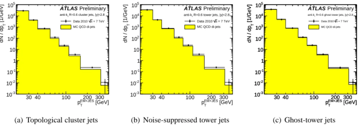
Figure 1 shows the jet pTjet distributions in Monte Carlo simulation and data for jets reconstructed using topological clusters as well as towers with and without noise suppression. All three jet types are calibrated using the EM+JES calibration scheme [10], with constants derived independently for each jet type (see Section 5).
[GeV]
T EM+JES
30 40 100 p200 300
[1/GeV]TdN / dp
10-3
10-2
10-1
1 10 102
103
104
105 ATLAS Preliminary
R=0.6 cluster jets, |y|<2.8 anti-kt
= 7 TeV s Data 2010 MC QCD di-jets
(a) Topological cluster jets
[GeV]
T EM+JES
30 40 100 p200 300
[1/GeV]TdN / dp
10-3
10-2
10-1
1 10 102
103
104
105 ATLAS Preliminary
R=0.6 tower jets, |y|<2.8 anti-kt
= 7 TeV s Data 2010 MC QCD di-jets
(b) Noise-suppressed tower jets
[GeV]
T EM+JES
30 40 100 p200 300
[1/GeV]TdN / dp
10-3
10-2
10-1
1 10 102
103
104
105
[GeV]
T EM+JES
30 40 100 p200 300
[1/GeV]TdN / dp
10-3
10-2
10-1
1 10 102
103
104
105 ATLAS Preliminary
R=0.6 ghost tower jets, |y|<2.8 anti-kt
= 7 TeV s Data 2010 MC QCD di-jets
(c) Ghost-tower jets
Figure 1: Transverse momentum (pT) distributions using the Monte Carlo-based pTandηjetcalibration for three different input constituents.
The agreement between data and Monte Carlo simulation decreases with increasing pTjetfor all three types of jets. This may reflect limitations of the description of the hard-scattering process provided by the Monte Carlo generator (PYTHIA). Approximately 20% more noise-suppressed tower jets pass the jet selection criteria compared to those built from noise-suppresed topological cluster jets. Furthermore, the multiplicity of ghost-tower jets exceeds that of those with noise-suppression by roughly 10%. These effects are also observed in the Monte Carlo simulation and their magnitude is also well reproduced by the simulation. This is related to differences in the calorimeter response for jets built of different constituents that occur primarily near the pTjet threshold of 20 GeV. These differences cause complications in the calculation of the calibration constants, which do not allow obtaining closure, and thus an appropriate calibration, with the calibration scheme. The effect is much more pronounced for ghost-tower jets, since the lack of noise-suppression creates a large bias near the threshold that the calibration constants cannot describe. The effects are thus electromagnetic-scale threshold effects, and could be removed by improved calibration and jet-energy scale determination. Residual differences related to the sensitivity
of the calibration constants to the pT thresholds can be removed by requiring that pTjetbe sufficiently far away from this threshold.
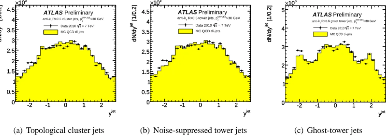
Figure 2 shows the rapidity (y) distribution in Monte Carlo simulation and data for jets with pTjet>
30 GeV and reconstructed using topological clusters as well as towers with and without noise sup- pression. The distributions are well described by the Monte Carlo simulation, even when no noise-
yjet
-2 -1 0 1 2
[1/0.2]jet dN/dy
0 0.5 1 1.5 2 2.5 3 3.5 4 4.5
103
×
yjet
-2 -1 0 1 2
[1/0.2]jet dN/dy
0 0.5 1 1.5 2 2.5 3 3.5 4 4.5
103
×
ATLAS Preliminary
>30 GeV T EM+JES R=0.6 cluster jets, p anti-kt
= 7 TeV s Data 2010 MC QCD di-jets
(a) Topological cluster jets
yjet
-2 -1 0 1 2
[1/0.2]jetdN/dy
0 0.5 1 1.5 2 2.5 3 3.5 4 4.5
103
×
yjet
-2 -1 0 1 2
[1/0.2]jetdN/dy
0 0.5 1 1.5 2 2.5 3 3.5 4 4.5
103
×
ATLAS Preliminary
>30 GeV T EM+JES R=0.6 tower jets, p anti-kt
= 7 TeV s Data 2010 MC QCD di-jets
(b) Noise-suppressed tower jets
yjet
-2 -1 0 1 2
[1/0.2]jet dN/dy
0 1 2 3 4 5
103
×
yjet
-2 -1 0 1 2
[1/0.2]jet dN/dy
0 1 2 3 4 5
103
×
ATLAS Preliminary
>30 GeV T EM+JES R=0.6 ghost tower jets, p anti-kt
= 7 TeV s Data 2010 MC QCD di-jets
(c) Ghost-tower jets
Figure 2: yjet distributions for jets above pTjet>30 GeV and for three different input constituents: (a) topological clusters, (b) towers with topological noise suppression and (c) towers without noise suppres- sion.
suppression is used. This validates the calorimeter noise description in the Monte Carlo simulation in the context of jets. A slight structure can be observed in the number of reconstructed jets as a function of yjet which is related to the jet reconstruction efficiency and the accuracy of the Monte Carlo-based calibration constants as a function of y. For jets built from towers without noise suppression, ghost-towers, the peak at|yjet| ≈2 corresponds to the transition from the barrel region to the end-cap hadronic calorimeters.
It again reflects inaccuracies in how the calibration constants capture the increased calorimeter response caused by increased noise. However, these features are reproduced by the Monte Carlo simulation.
The overall good agreement between data and Monte Carlo simulation reflects the good description of noise in the context of jets, jet reconstruction efficiencies and jet energy scale in the simulation.
4 Jet Properties and Internal Structure
In this section, we present studies of the objects used for jet finding and calibration (towers and clusters).
These observations are extended to include charged particle distributions within jets and the presence of close-by jets for multi-jet events. Finally, the longitudinal and transverse structure of jets is measured using both calorimeter-based objects and, in the case of the transverse structure, tracks. These mea- surements are used to study the presence of both physics and detector effects in the jet reconstruction and global jet properties. Results describing the jet properties observed in proton-proton collisions at a center-of-mass energy of 900 GeV are shown in Ref. [11].
4.1 Jet Constituent Properties
A good understanding of jet reconstruction requires the characterization of the inputs to jet reconstruc- tion inside the jets they form. This section presents distributions of the multiplicity of the constituents inside jets. Comparisons of these distributions between Monte Carlo simulations and data aid in deter-
mining how well the generated particle spectra and the detector simulation describe the formation of the constituent objects in the context of a jet.
Figure 3 shows the number of topological clusters and noise-suppressed towers inside jets built of these constituents, as well as the variation as a function of yjet. Since towers have a size of ∆η×
∆φ =0.1×0.1, the maximum number of constituents expected in these jets, from a purely geometrical argument, is Ntowers≈113 (assuming a perfect jet cone with radius R=0.6). The distribution shows that jets contain many fewer towers when noise suppression is applied, with a mean ofhNtowersi ≈44 for central jets (|yjet|<0.3, Fig. 3) . The mean number of topological clusters per jet is roughly one quarter of the mean number of towers, hNclustersi ≈13, for central jets. The smaller number of topological clusters is expected, given that the clustering algorithm attempts to incorporate the hadronic shower of one particle in one cluster.
For both input constituent types, the overall shape of the multiplicity distribution is well described by the Monte Carlo simulation. However, in both cases, a shift is observed in the comparison leading to a 6.4% (4.0%) deficiency in the Monte Carlo simulation for towers (clusters). The discrepancy between data and Monte Carlo simulation is larger for topological clusters in the transition region between the barrel and end-cap calorimeters, whereas the difference is roughly constant for jets built from towers.
The difference in the trend of the multiplicity distributions at high-yjet– where the tower multiplicity per jet increases yet the cluster multiplicity decreases – is another feature of the difference in definition of these inputs. Since the towers follow a projective geometrical definition, the physical size of each tower changes with y, while the topological cluster definition follows the shower development. In the forward region, hadronic showers are large with respect to the tower size. As a result, it is more difficult to separate showers from individual particles in the forward regions of the detector.
4.2 Properties of Tracks in Jets
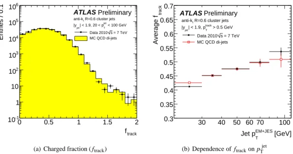
The ID provides precise measurements of the momentum of charged particles emerging from the pp collisions which in turn yield information regarding the fraction of neutral and charged energy contained in the jet and the internal jet structure. Measurements of the track multiplicity in jets, Ntrack, and its correlation with pTjet using the simple∆R<0.6 matching criterion are presented, where the matching is performed using the track coordinates at the perigee without extrapolating them to the surface of the calorimeter. The total scalar sum of track momenta associated with a jet,∑pTtrack, can be used to provide further details on the calorimeter response to jets. The ratio of∑pTtrackto pTjet, referred to as ftrack, can be used after the jet calibration in order to improve the jet energy resolution, as demonstrated in Monte Carlo simulations [9]. For all distributions, the Monte Carlo simulations have been normalized to the number of jets present in the data. In this section, jets are selected with|yjet|<1.9, to account for the ID coverage (|ηtrack|<2.5) and the requirement that tracks be contained within a cone of radius R=0.6 around the jet axis. Jets are also required to have transverse momenta within the range 20<pTjet<100 GeV so that uncertainties related to tracking efficiency in higher pTjets do not impact these studies.
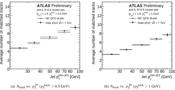
Figure 4 shows the measured number of tracks inside jets and Figure 5 the variation of Ntrackwith pTjet, in each case for jets built from topological clusters and repeated for tracks with pTtrack>0.5 GeV and 1 GeV. The measurements are nearly identical for jets built from noise-suppressed towers, and are thus omitted for brevity. The track multiplicity is peaked at Ntrack =4 (Ntrack =3) with a mean of hNtracki=5.0 (hNtracki=3.5) for pTtrack>0.5 GeV (pTtrack >1 GeV). As expected, hNtracki increases with increasing pTjet.
The measurements indicate that the Monte Carlo simulation underestimates the number of tracks in a jet by roughly 5% across a large range in pTjet in the case of the 0.5 GeV pTtrack selection. This discrepancy is greatly reduced by increasing the track selection to 1 GeV. Even when restricting the measurement to the very central region of the calorimeter (|yjet|<0.3) the discrepancy at low-pTtrack
Number of constituents
0 20 40 60 80 100 120
Number of jets
0 1 2 3 4 5 6 7 8 9
103
×
ATLAS Preliminary
R=0.6 tower jets anti-kt
| < 0.3
|yjet
MC QCD di-jets = 7 TeV s Data 2010
(a) Number of towers per jet
Number of constituents 0 5 10 15 20 25 30 35 40
Number of jets
0 1 2 3 4 5 6 7 8 9
103
×
ATLAS Preliminary
R=0.6 cluster jets anti-kt
| < 0.3
|yjet
MC QCD di-jets = 7 TeV s Data 2010
(b) Number of clusters per jet
Jet yjet
-2 -1 0 1 2
Mean number of constituents
20 40 60 80 100
120 ATLAS Preliminary
R=0.6 tower jets anti-kt
MC QCD di-jets = 7 TeV s Data 2010
(c) Number of towers vs. yjet
Jet yjet
-2 -1 0 1 2
Mean number of constituents
10 12 14 16 18 20 22 24 26
28 ATLAS Preliminary
R=0.6 cluster jets anti-kt
MC QCD di-jets = 7 TeV s Data 2010
(d) Number of clusters vs. yjet
Figure 3: Number of constituents (top) in jets built with noise-suppressed towers (left) and topological clusters (right), compared between data and Monte Carlo simulation for central jets (|yjet|<0.3). The variation of the constituent multiplicity as a function of yjetis also shown (bottom).
remains. As will be shown in both the transverse jet structure and the jet shapes (Section 4), this is one of several indications of potentially imperfect tuning of the Monte Carlo simulation. Other studies [12]
indicate that the detector simulation models well properties of tracks in jets while the fragmentation function and underlying event used by the Monte Carlo generator may require further tuning [13].
The measured ftrack distribution is shown in Figure 6 for jets built from topological clusters and indicates a 3-4% higher mean value predicted from the Monte Carlo simulation compared to the data for the inclusive y selection (the same effect is seen for noise-suppressed tower jets). When restricting the jets to be within|yjet|<0.3 or above pTjet>30 GeV (or both) this difference vanishes, suggesting that the discrepancy is primarily localized in the low-pT range and slightly more forward directions. This difference is well within the total jet-energy scale uncertainty [10].
Number of matched tracks 0 2 4 6 8 10 12 14 16 18
Number of jets
5 10 15 20 25 30 35 40 45
103
×
ATLAS Preliminary
R=0.6 cluster jets anti-kt
< 100 GeV T
EM+JES
| < 1.9, 20 < p
|yjet > 0.5 GeV T track p
MC QCD di-jets = 7 TeV s Data 2010
(a) Track multiplicity (pTtrack>0.5 GeV)
Number of matched tracks 0 2 4 6 8 10 12 14 16 18
Number of jets
10 20 30 40 50 60
103
×
ATLAS Preliminary
R=0.6 cluster jets anti-kt
< 100 GeV
T EM+JES
| < 1.9, 20 < p
|yjet
> 1.0 GeV
T track
p
MC QCD di-jets = 7 TeV s Data 2010
(b) Track multiplicity (pTtrack>1 GeV)
Figure 4: Distribution of the number of charged tracks (Ntrack) matched to the calorimeter jet for both (a) the nominal pTtrack>0.5 GeV requirement and (b) an increased pTtrack>1 GeV selection.
[GeV]
EM+JES
Jet pT
30 40 50 60 70 80 100
Average number of matched tracks
0 2 4 6 8 10 12
14 ATLAS Preliminary
R=0.6 cluster jets anti-kt
> 0.5 GeV
T track
| < 1.9, p
|yjet
MC QCD di-jets = 7 TeV s Data 2010
(a) Ntrackvs. pTjet(pTtrack>0.5 GeV)
(GeV)
EM+JES
Jet pT
30 40 50 60 70 80 100
Average number of matched tracks
0 2 4 6 8 10 12
14 ATLAS Preliminary
R=0.6 cluster jets anti-kt
> 1 GeV
T track
| < 1.9, p
|yjet
MC QCD di-jets = 7 TeV s Data 2010
(b) Ntrackvs. pTjet(pTtrack>1 GeV)
Figure 5: Correlation of the number of charged tracks (Ntrack) matched to the calorimeter jet with pTjet for both (a) the nominal pTtrack>0.5 GeV requirement and (b) an increased pTtrack>1 GeV selection.
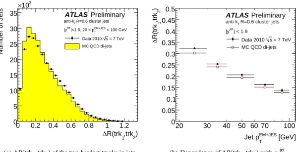
4.3 Close-By Jets
The distance between two reconstructed jets can have a large impact both on the jet properties and the resulting jet calibration and achievable jet energy scale precision. A very close second jet can result in large energy sharing between the jets that is not accounted for in jet calibration schemes that typically rely on isolated final state objects. Figure 7 depicts measurements in data and Monte Carlo simulation of the smallest distance in∆R between a reconstructed jet of either 20<pTjet<30 GeV or 40<pTjet<60 GeV and the closest jet with pEMScaleT >7 GeV (i.e. pTjetprior to calibration, which corresponds to∼10 GeV at the calibrated scale) for jets built from topological clusters.
track
f
0 0.5 1 1.5 2
Entries / 0.1
10-1
1 10 102
103
104
105
106
ATLAS Preliminary
R=0.6 cluster jets anti-kt
< 100 GeV
T
| < 1.9, 20 < pjet
|yjet
= 7 TeV s Data 2010 MC QCD di-jets
(a) Charged fraction ( ftrack)
[GeV]
EM+JES
Jet pT
30 40 50 60 70 100
trackAverage f
0.3 0.35 0.4 0.45 0.5 0.55 0.6 0.65 0.7
ATLAS Preliminary
R=0.6 cluster jets anti-kt
> 0.5 GeV
T track
| < 1.9, p
|yjet
= 7 TeV s Data 2010 MC QCD di-jets
(b) Dependence of ftrackon pTjet
Figure 6: (a) Distribution of the charged particle fraction, ftrack, for calorimeters jets built from topolog- ical clusters and (b) its correlation with pTjet. The same trends are observed for noise-suppressed tower jets.
Rmin
0 1 2 3 4 5 ∆ 6
Number of Jets/0.2
0 5 10 15 20 25 30 35
103
×
R=0.6 cluster Jets anti-kt
<30 GeV
T EM+JES
|y|<2.8, 20 GeV<p
ATLAS Preliminary
=7 TeV s Data 2010 MC QCD di-jets
(a) 20<pTjet<30 GeV
Rmin
0 1 2 3 4 5∆ 6
Number of Jets/0.2
0 0.5 1 1.5 2 2.5 3
103
×
R=0.6 cluster Jets anti-kt
<60 GeV
T EM+JES
|y|<2.8, 40 GeV<p
ATLAS Preliminary
=7 TeV s Data 2010 MC QCD di-jets
(b) 40<pTjet<60 GeV
Figure 7: Minimum distance in∆R=p
∆η2+∆φ2to a jet with pEMScaleT >7 GeV for cluster jets with
|yjet|<2.8 and (a) 20<pTjet<30 GeV or (b) 40<pTjet<60 GeV.
Most important is the component of the distribution with∆R<1.5 which implies the presence of a very close second jet. An excess of such close-by jets is observed in the data above that predicted by the Monte Carlo simulation. This excess becomes larger as the cut on the closest jet pEMScaleT becomes smaller, and it becomes smaller as the pTof the jet in consideration increases. This behavior appears con- sistently for all rapidities up to|yjet|=2.8, and has also been observed for jets built of noise-suppressed towers.
The implications of this effect are a possible increase in the jet energy scale systematic error, a broadening of the jet resolution and differences in the internal jet structure. The calorimeter response for non-isolated jets in the Monte Carlo simulation has been shown to be lower than for isolated jets [10], and an increase in jets of this kind motivates the need for a jet energy scale correction dependent on∆Rmin. Such a correction would remove biases in the response in the data and in the Monte Carlo simulation, independent of disagreements on the rates between data and Monte Carlo simulation.
4.4 Longitudinal and Transverse Jet Profiles
Hadronic shower development within the calorimeter and its modeling by the detector simulation play an integral role in understanding the application of jet calibration techniques. In this section, we focus on comparing some of the distributions characterizing transverse and longitudinal jet properties on which many calibration schemes depend in data and Monte Carlo simulations. In many cases, only representa- tive distributions are shown for brevity.
4.4.1 Longitudinal Profile
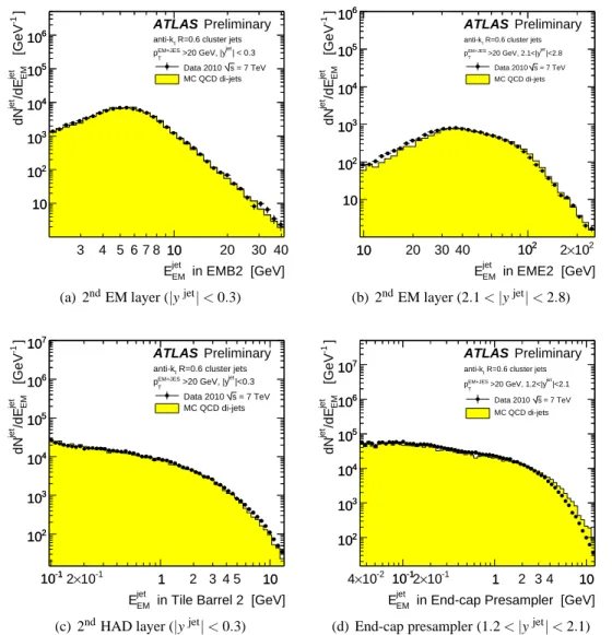
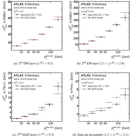
Figure 8 shows the distributions of energies deposited by topological cluster jets in four of the longitu- dinal segments of the calorimeters with the requirement that pTjet>20 GeV. Figure 9 presents the mean of these distributions as a function of the pTjet. A reasonable agreement is observed not only in the bar- rel region (|yjet|<0.3) for both the electromagnetic and hadronic calorimeters, but also in the end-cap (2.1<|yjet|<2.8) where the average energy deposit is more than an order of magnitude larger. This agreement persists over the entire range of jet pTjetprobed in this study, except potentially for the highest pT jets in the end-cap, where the statistics are currently low. Other layers and rapidity ranges show no significant deviations, with the exception of the gap scintillators and the end-cap presampler (Fig. 9(d)), the former being used to provide signals to aid in correcting for energy losses in the inactive material in the gap. In both of these cases, slight excesses are observed at low E and deficiencies at high E. This results in a lower mean energy deposition in these layers in the data than predicted by the Monte Carlo simulation across the full range of pTjet. These discrepancies are related to the EM-scale calibration of these components, particularly in the case of the gap scintillators [14].
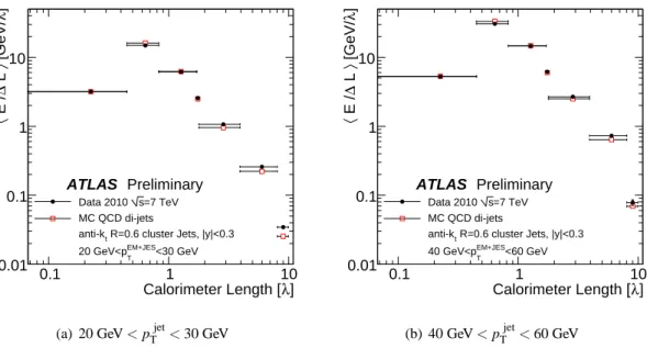
In order to more closely study the actual shower development in terms of the number of absorption lengths traversed by the particles in the jet, Figure 10 shows the mean value of the energy deposited in the different longitudinal segments per absorption length as a function of the number of absorption lengths traversed by the jet. The thin layer atλ ≈2 corresponds to the third layer of the electromagnetic calorimeter. These longitudinal profiles are measured for central jets built from topological clusters with a transverse momentum between 20 GeV<pTjet<30 GeV and 40 GeV<pTjet<60 GeV and compared to the Monte Carlo simulation. A larger longitudinal energy density is observed in the Monte Carlo simulation than in the data in the first layer of the electromagnetic calorimeter, while a good agreement in the density in the other layers of the electromagnetic calorimeter and the presampler is observed between data and Monte Carlo simulation. A smaller energy density is observed in the Monte Carlo simulation than in the data in the three last points, corresponding to the hadronic calorimeter segments.
This seems to indicate that, at least in the barrel, the hadronic shower is deeper in data than in the Monte Carlo simulation.
3 4 5 6 7 8 10 20 30 40 10
102
103
104
105
106
in EMB2 [GeV]
EM
Ejet
10 ]-1 [GeVEM
jet /dEjet dN
10 102
103
104
105
106
ATLAS Preliminary
R=0.6 cluster jets anti-kt
| < 0.3 >20 GeV, |yjet EM+JES pT
= 7 TeV s Data 2010 MC QCD di-jets
(a) 2ndEM layer (|yjet|<0.3)
10 20 30 40 102 2×10² 10
102
103
104
105
106
in EME2 [GeV]
EM
Ejet
10 102
]-1 [GeVEM
jet /dEjet dN
10 102
103
104
105
106
ATLAS Preliminary
R=0.6 cluster jets anti-kt
|<2.8 >20 GeV, 2.1<|yjet EM+JES T p
= 7 TeV s Data 2010 MC QCD di-jets
(b) 2ndEM layer (2.1<|yjet|<2.8)
10-12×10-1 1 2 3 4 5 10 102
103
104
105
106
107
in Tile Barrel 2 [GeV]
EM
Ejet
10-1 1 10
]-1 [GeVEM
jet /dEjet dN
102
103
104
105
106
107
ATLAS Preliminary
R=0.6 cluster jets anti-kt
|<0.3 >20 GeV, |yjet EM+JES T
p
= 7 TeV s Data 2010 MC QCD di-jets
(c) 2ndHAD layer (|yjet|<0.3)
10-2
×
4 10-12×10-1 1 2 3 4 10 102
103
104
105
106
107
in End-cap Presampler [GeV]
EM
Ejet
10-1 1 10
]-1 [GeVEM
jet /dEjet dN
102
103
104
105
106
107
ATLAS Preliminary
R=0.6 cluster jets anti-kt
|<2.1 >20 GeV, 1.2<|yjet EM+JES
pT
= 7 TeV s Data 2010 MC QCD di-jets
(d) End-cap presampler (1.2<|yjet|<2.1)
Figure 8: Example distributions of energy deposited by jets with pTjet>20 GeV in layers of the calorime- ter compared to that predicted from Monte Carlo simulation for (a) the second layer of the electromag- netic calorimeter in the central region, (b) the second layer of the electromagnetic calorimeter in the end-cap, (c) the second layer of the hadronic calorimeter in the central region, and (d) the end-cap pre- sampler layer.
4.4.2 Transverse Jet Profile
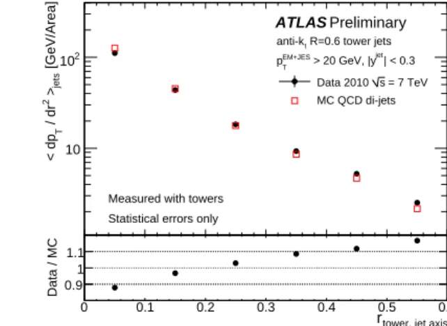
The transverse profile of the jet can be characterized in terms of the jet width, wjet, defined as the weighted average distance of the jet constituents to the jet direction,
wjet = ∑
constituents
(r×ETi)/ ∑
constituents
ETi,where (3)
r =
q(φi−φjet)2+ (ηi−ηjet)2, (4) and ETi is the transverse energy of the jet constituent (tower or cluster), and the sum runs over all con- stituents comprising the jet. Figure 11 shows the measured jet width distribution for an inclusive selec- tion of jets built from topological clusters within|y|<2.8 and pTjet>20 GeV. Although the spread of the