The overview of the ATLAS local hadronic calibration.
Guennadi Pospelov, for the ATLAS hadronic calibration group.
Max-Planck-Institut f¨ ur Physik, Werner-Heisenberg-Institut F¨ ohringer Ring 6, 80805 Munich, Germany
E-mail: pospelov@mppmu.mpg.de
Abstract.
We present the concept of the local hadronic calibration for the ATLAS calorimeter system as a tool to get calibrated jets at particle level for any jet algorithm. The procedure is based on detailed Geant4 simulations providing information on energy deposits in all parts of the ATLAS detector. Calibration starts from topological clusters reconstructed and calibrated at the electromagnetic scale. First classification step tags clusters as mainly electromagnetic, or hadronic depending on cluster shape variables. Clusters which are identified as being electromagnetic are kept at the electromagnetic scale. Hadronic clusters receive cell weights to correct for the invisible energy deposits of hadrons. Next steps are out-of-cluster corrections for lost energy deposited in calorimeter cells outside of reconstructed clusters and dead material corrections for energy deposited outside of active calorimeter volumes. Finally out-of-jet corrections are applied to get the final jet energy scale.
1. Introduction
The jet energy scale is one of the main systematic uncertainties in many physics studies foreseen with the ATLAS detector [1]. Top mass reconstruction or measurements of inclusive jet cross-section are examples relevant for the first data taking phase. The initial parton energy differs from the energy of the hadronic shower because of detector effects, like calorimeter non- compensation and energy losses in dead material, jet effects, like bending of secondary particles out of the jet cone by the magnetic field or jet reconstruction algorithm specifics, and effects from the collision physics environment.
In this paper we present the concept of the local hadronic calibration for jets to the particle level independent on any jet algorithm. The ultimate goal of the procedure is to provide jet algorithms with constituents — calibrated clusters with energies corresponding to the stable particle energies. The key feature of the approach is to factorize corrections in several sequential steps to disentangle detector effects of different types and to correct them independently.
Starting point for the local hadronic calibration is topological clustering [2] in the calorimeter
cells which have been calibrated at the electromagnetic (em) scale. Cluster shape variables are
then used to classify clusters as having electromagnetic or hadronic nature. The hadron-like
clusters are subject of a cell weighting procedure to compensate for the lower responce of the
calorimeter to hadronic deposits, while clusters classified as electromagnetic-like, are kept at the
original scale. Next out-of-cluster (OOC) corrections for lost energy deposited in calorimeter cells
outside of reconstructed clusters in the tail of hadronic shower are applied. Finally, dead material
, GeV
π-
E
104 105 106
-π / EfracE
0 0.1 0.2 0.3 0.4 0.5 0.6 0.7 0.8 0.9 1
Figure 1. Calibration energy fractions ( • - visible em, ◦ - visible non-em,
- invisible,
N - escaped) released in active and inactive material in the endcap region (1.5 < | η | <
3.0) by single charged pions vs. the pion energy.
η
0 0.5 1 1.5 2 2.5 3 3.5 4 4.5 5
) energy / True Pion Energy•),DM(°OOC(
0 0.05 0.1 0.15 0.2 0.25 0.3 0.35 0.4
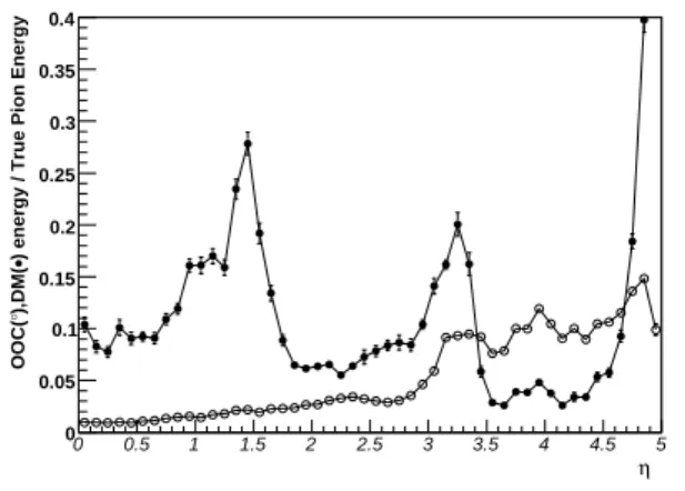
Figure 2. Fractions of true calibra- tion hit energies outside topological clusters but inside the calorimeters ( ◦ ) and outside calorimeters ( • ) as function of pion pseudo- rapidity for 200 GeV pion energy.
(DM) corrections are applied on the cluster level to account for energy deposits outside of active calorimeter volumes, e.g. in the cryostat, the magnetic coil and calorimeter intermodular cracks.
To derive the correction coefficients for all calibration steps we use actual energy deposits in active and inactive volumes known from detailed Geant4 [3] simulations via the so-called calibration hits mechanism.
2. Simulation and Calibration Hits
The classification and calibration methods described in this paper are based on detailed simulations of single pions in the standard ATLAS environment. The data set consist of 10 6 neutral and 2 · 10 6 charged pions with initial η, φ coordinates randomly distributed across the entire detector. The initial pion energies were generated in 1000 logarithmically equidistant steps from 150 MeV to 2 TeV.
Calibration hits provide access to the energy deposits in active (liquid argon, scintillator), inactive (absorber) and dead material regions for the following four categories of energy deposits:
• visible em-energy: The energy released by electrons or positrons via ionization.
• visible non-em-energy: The energy released by charged particles other than electrons or positrons via ionization.
• in-visible energy: The energy released by non-ionizing processes such as break-up of nuclear bindings.
• escaped energy: The energy leaving the mother volume in form of non-interacting or escaping particles like neutrinos or muons.
Figure 1 shows the average fraction of each of these 4 categories summed over the active and inactive regions in the endcap calorimeters as a function of the pion energy. Error bars on the figure represent rms values. Figure 2 shows the total out-of-cluster and dead material energy fractions known from calibration hits as function of pion pseudorapidity for 200 GeV charged pions.
The aim of the calibration is to reconstruct the lost invisible and escaped energy on an
event-by-event basis with measured energy depositions inside calorimeter cells.
(MeV)) )) - log10(Eclus
> (MeV/mm3 ρcell
log10(<
-9 -8.5 -8 -7.5 -7 -6.5 -6 -5.5 -5 -4.5 -4 (mm))clusλlog10(
0 0.5 1 1.5 2 2.5 3 3.5 4
0 0.1 0.2 0.3 0.4 0.5 0.6 0.7 0.8 0.9 1
Figure 3. Probability weights to observe a neutral pion cluster for 8 GeV < E cluster <
16 GeV.
(MeV)) log10(Eclus
2 2.5 3 3.5 4 4.5 5 5.5 6
))3 (MeV/mm cellρlog10(
-7 -6 -5 -4 -3 -2 -1 0 1
reco/EtotE
0 0.2 0.4 0.6 0.8 1 1.2 1.4 1.6 1.8 2
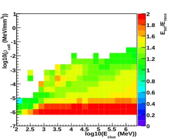
Figure 4. Hadronic cell weights for Tile barrel sampling 1 at 0.2 < | η | < 0.4.
3. Local Hadronic Calibration 3.1. Cluster Classification
Aim of the cluster classification is to distinguish between clusters seeded by electromagnetic or hadronic interactions. For topological clusters where the correspondence of cluster and particle level is close this would lead to a separation of electrons, photons and neutral pions on one side from charged hadrons (mainly pions) and neutrons on the other side such that both particle classes can be optimally calibrated.
The current default procedure in ATLAS is to classify topological clusters basing on the predicted phase-space population of clusters stemming from charged and neutral pion simulations. The separation of hadronic from electromagnetic showers relies on the following cluster shape variables: the average cell energy density h ρ i and the depth of the shower center λ center . For both particle species the 4-dimensional phase space for clusters in | η | , E cluster , log 10 (λ center ) and log 10 ( h ρ i ) − log 10 (E cluster ) is binned and filled with simulated pions in the energy range E cluster = 200 MeV − 2 TeV and | η | < 5. Assuming an a-priori probability ratio of 1 : 2 for observing a neutral pion over a charged pion the probability weight in each phase-space bin for observing a neutral pion is given by: w i = n π i
0/(n π i
0+ 2n π i
±), where n π i
0,±is the fraction of clusters at given energy and η of neutral or charged pions in a given phase-space bin i from the simulation. A cluster is classified as electromagnetic if the lookup value for w i > 0.5 at a given cluster phase-space bin.
Figure 3 shows the classification weights obtained with this procedure for the region 0.2 <
| η | < 0.4 and 8 GeV < E cluster < 16 GeV on a colored scale from 0 (purely hadronic) to 1 (purely electromagentic as a function of the two moments h ρ i and λ center . It is clearly visible that electromagnetic showers dominate the region of high energy density and small cluster depth.
It is also apparent from the plots that classification is most difficult for clusters with smaller energies as the distributions for charged and neutral pions have larger overlaps in that regime.
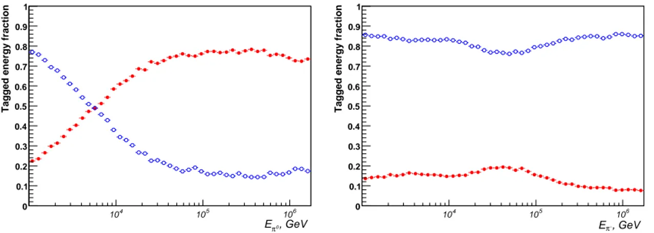
The classification performance in terms of the energy fractions classified as electromagnetic
and hadronic for neutral and charged single pions is shown in figure 5. For neutral pions the
method reaches classification efficiencies of 80 − 85% above 50 GeV, but below that energy the
electromagnetic fraction drops linearly with the logarithm of the pion energy. For charged pions
the hadronic fraction is rather stable between 80 − 90% over the entire energy range – at low
energies due to the low classification efficiency of neutral pions and at large energies due to the
better separation of neutral and charged showers.
, GeV
π0
E
104 105 106
Tagged energy fraction
0 0.1 0.2 0.3 0.4 0.5 0.6 0.7 0.8 0.9 1
, GeV
π-
E
104 105 106
Tagged energy fraction
0 0.1 0.2 0.3 0.4 0.5 0.6 0.7 0.8 0.9 1
Figure 5. Energy fractions of single pions classified as electromagnetic ( • ) or hadronic ( ◦ ) for π 0 ’s (left), π ± ’s (right) as function of the pion energy averaged over all η and φ.
3.2. Cluster Weighting
For clusters classified as hadronic a H1-type cell-based weighting procedure [4, 5] is applied to correct for invisible and escaped energy fractions. The weight tables are filled with the ratios E calib
cell /E reco
cell , where E reco
cell is the regular simulated energy based on the visible energy in the active media including noise, while E calib
cell is the sum of the four calibration energies deposited in the given cells active and inactive parts. Average weights are kept as a function of the cluster energy the cell belongs to, the energy density ρ cell = E reco
cell /V cell of the cell, and the
| η | of the cell center. There are 25 equidistant | η | -bins from 0.0 to 5.0, 20 logarithmic energy- density bins from − 7 < log 10 (ρ cell(MeV /mm 3 )) < 1 and 22 logarithmic cluster energy bins from log 10 (100(MeV)) < log 10 (E clus(MeV)) < log 10 (2 · 10 6 (MeV)). Examples of the actual weights for the first sampling of the Tile calorimeter obtained this way from 2 · 10 6 charged pions are shown in figure 4.
3.3. Out-of-Cluster corrections
Out-of-cluster corrections aim for recovering from the lost low energetic deposits at the tails of hadronic showers. This energy is deposited in calorimeter cells which are not part of any reconstructed cluster due to noise thresholds in the clustering.
The total fraction of out-of-cluster energy from single pion simulations w.r.t. the weighted total energy inside clusters is averaged in bins of pion energy, pion | η | , and the pion depth λ in the calorimeter. The λ values of all clusters in a given event are combined with energy proportional weights to obtain the latter. 12 energy bins with the boundaries { 0, 1, 2, 4, 8, 16, 32, 64, 128, 256, 512, 1024, 2048 } GeV, 25 equidistant | η | bins from 0 to 5 and 20 equidistant bins in log 10 (λ/mm) from 0 to 4 define the lookup table.
However, out-of-cluster energy estimated with the help of tables of that kind turned out to
be overrated in multi particle event. This is due to the fact, that energy which is outside of one
cluster could actually be inside the other cluster. To resolve this problem the level of isolation of
clusters is used [6]. It is determined by the fraction of cells on its outer perimeter not included
in other clusters. An isolation of 0 means that all cells on its outer perimeter are included in
neighboring clusters, a value of 1 indicates that the cluster is totally isolated – i.e. that all its
neighbor cells are not part of any cluster. This isolation fraction is multiplied with the expected
out-of-cluster energy fraction for each cluster as obtained from the out-of-cluster tables described
above. This accounts for the fact that clusters tend to be less isolated in full events compared
to single pion events from simulations or beam tests.
η
0 0.5 1 1.5 2 2.5 3 3.5 4 4.5 5
DM area energy / Total DM energy
0 0.2 0.4 0.6 0.8 1
Figure 6. Ratio of energy deposited in different DM regions ( • - before em calorimeter, ◦ - between em and had,
- intermodular cracks,
- leakages, N - before forward calorimeter) to the total DM energy for charged pion with energy 200 GeV.
* E
HEC0E
EME30 5000 10000 15000 20000 25000 30000 35000 40000
E(dead material), MeV
0 2000 4000 6000 8000 10000 12000
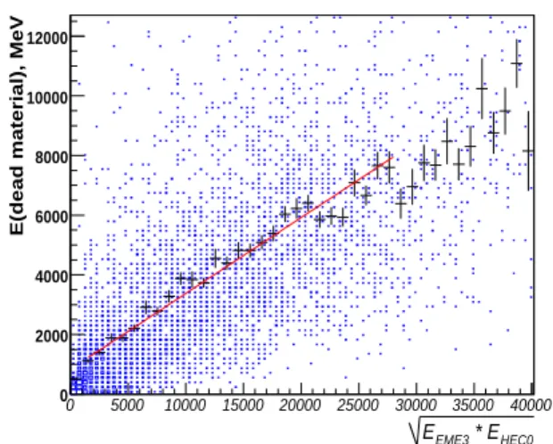
Figure 7. Dependence of energy deposited between em and had endcap calorimeters on
√ E EM E3 · E H EC0 , where E EM E3 energy in last em sampling, E H AD0 energy in first had samplings.
3.4. Dead material corrections
Dead material corrections are accounting for energy deposited outside of active zones of the electromagnetic and hadronic calorimeters. This includes energy deposited in upstream material (Inner Detector material, magnetic coil, cryostat walls), different crack regions between calorimeter modules and material behind calorimeter system (leakages). Figure 6 shows the ratio of energy deposited in different DM regions to the total DM energy for charged pions with 200 GeV energy as a function of the pion pseudorapidity. These regions are treated variously to get and to apply DM correction coefficients. For upstream material the good correlations of DM deposits with the preshower signals are used. Deposits between electromagnetic and hadronic calorimeters are corrected for by weighting the geometric average of signals in the last em and first had sampling. (see figure 7). Correction coefficients then are parametrised as a function of cluster energy and pseudorapidity. For intricate DM regions where there are no cluster quantitities correlating well with DM energy deposits, 3 dimensional lookup tables on E cluster , η cluster , λ cluster are used to store average ratios of DM energy to the cluster energy.
4. Performance
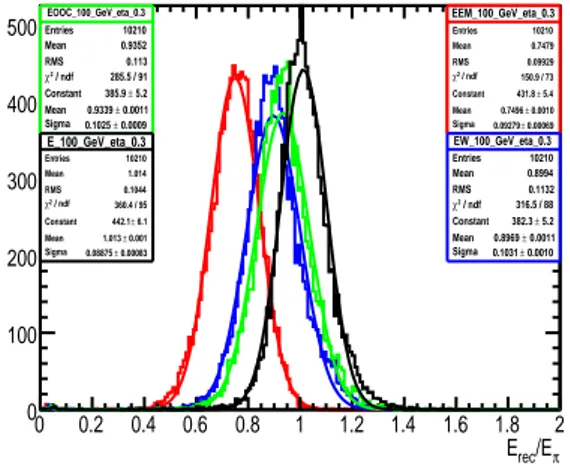
Figure 8 shows the ratio of reconstructed over simulated pion energy at the em-scale, and after applying 3 sequential steps of local hadronic calibration: hadronic weighting, out-of-cluster and dead material corrections. The plot has been obtained for 100 GeV single charged pions in the region 0.2 < | η | < 0.4. It is clearly seen that each step shifts the mean of the reconstructed energy toward the truth energy and, at the end, gives the correct value. The energy resolution is improving on each step as well.
The performance of local hadronic calibration on di-jet events is presented in figure 9. Jets
are formed by the K T jet algorithm with R = 0.6 from topological clusters, calibrated with the
local hadronic calibration scheme, and compared to the truth matched jets. Thus, for the barrel
and endcap regions the local hadronic calibration recovers linearity for 100 GeV jets up to 92%,
while for 10 GeV jets missed energy reaches 25%. Main sources of remaining energy correction
and their impact on the energy underestimation are presented below (calculation has been done
EEM_100_GeV_eta_0.3
Entries 10210
Mean 0.7479
RMS 0.09929
/ ndf
χ2 150.9 / 73
Constant 431.8 ± 5.4 Mean 0.7496 ± 0.0010 Sigma 0.09279 ± 0.00069
/E
πE
rec0 0.2 0.4 0.6 0.8 1 1.2 1.4 1.6 1.8 2
0 100 200 300 400
500
EEM_100_GeV_eta_0.3Entries 10210
Mean 0.7479
RMS 0.09929
/ ndf
χ2 150.9 / 73
Constant 431.8 ± 5.4 Mean 0.7496 ± 0.0010 Sigma 0.09279 ± 0.00069 EW_100_GeV_eta_0.3
Entries 10210
Mean 0.8994
RMS 0.1132
/ ndf
χ2 316.5 / 88
Constant 382.3 ± 5.2 Mean 0.8969 ± 0.0011 Sigma 0.1031 ± 0.0010 EOOC_100_GeV_eta_0.3
Entries 10210
Mean 0.9352
RMS 0.113
/ ndf
χ2 285.5 / 91
Constant 385.9 ± 5.2 Mean 0.9339 ± 0.0011 Sigma 0.1025 ± 0.0009 E_100_GeV_eta_0.3
Entries 10210
Mean 1.014
RMS 0.1044
/ ndf
χ2 360.4 / 95
Constant 442.1 ± 6.1 Mean 1.013 ± 0.001 Sigma 0.08875 ± 0.00083
Figure 8. The ratio of reconstructed over simulated pion energy at various stages of the calibration.
(GeV)
truth
E
10
210
3truth/Ejet E
0.75 0.8 0.85 0.9 0.95 1 1.05 1.1
ATLAS
< 0.4
|η|
Kt6 LC/MC jets 0.2 <
< 2.2
|η|
Kt6 LC/MC jets 2 <