ATLAS NOTE
March 28, 2008
Calibration model for the MDT chambers of the ATLAS Muon Spectrometer
P. Bagnaia11, T. Baroncelli12, O. Biebel8, C. Bini11, S. Borroni11, P. Celio12, M. Cirilli6, M. Curti11, A. De Salvo11, M. Deile8,∗, S. Di Luise12, A. Di Mattia7, E. Diehl6, G. Dimitrov1, J. Dubbert9, G. Duckeck8, S. Falciano11, S. Gadomski5,3, P. Gauzzi11, M. Groh9, R. Hertenberger8, N. Hessey8,∗∗, S. Horvat9, M. Iodice12, S. Kaiser9, O. Kortner9, H. Kroha9, S. Kolos2, D. Levin6, L. Luminari11, B. Martin2, S. McKee6, D. Merkl8, D. Orestano12, E. Pasqualucci11, F. Petrucci12, L. Pontecorvo11, I. Potrap9, F. Rauscher8, S. Rosati11, E. Solfaroli Camillocci11, L. Spogli12, R. Stroehmer8, F. Tique Aires Viegas2, M. Verducci2, E. Vilucchi4, N. van Eldik10,∗∗∗, Z. van Kesteren10, J. von Loeben9, M. Woudstra10,∗∗∗, B. Zhou6
Corresponding author: Domizia.Orestano@cern.ch
1Lawrence Berkeley National Laboratory and University of California, Physics Division, MS50B-6227, 1 Cy- clotron Road, Berkeley, CA 94720, United States of America
2CERN, CH - 1211 Geneva 23, Switzerland, Switzerland
3The Henryk Niewodniczanski Institute of Nuclear Physics, Polish Academy of Sciences, ul. Radzikowskiego 152, PL - 31342 Krakow, Poland
4INFN Laboratori Nazionali di Frascati, via Enrico Fermi 40, IT-00044 Frascati, Italy
5Universit´e de Geneve, Section de Physique, 24 rue Ernest Ansermet, CH - 1211 Geneve 4, Switzerland
6The University of Michigan, Department of Physics, 2477 Randall Laboratory, 500 East University, Ann Arbor, MI 48109-1120, United States of America
7Michigan State University, High Energy Physics Group, Department of Physics and Astronomy, East Lansing, MI 48824-2320, United States of America
8Fakult¨at f¨ur Physik der Ludwig-Maximilians-Universit ¨at M¨unchen, Am Coulombwall 1, DE - 85748 Garching, Germany
9Max Planck Institut f ¨ur Physik, Postfach 401212, Foehringer Ring 6, DE - 80805 M ¨unchen, Germany
10Nikhef National Institute for Subatomic Physics, Kruislaan 409, P.O. Box 41882, NL - 1009 DB Amsterdam, Netherlands
11INFN Roma and Universit `a La Sapienza, Dipartimento di Fisica, Piazzale A. Moro 2, IT- 00185 Roma, Italy
12INFN Roma Tre and Universit `a di Roma Tre, Dipartimento di Fisica, via della Vasca Navale 84, IT-00146 Roma, Italy
∗Now at CERN
ATL-MUON-PUB-2008-004 28 March 2008
∗∗Now at Nikhef
∗∗∗Now at Department of Physics, University of Massachusetts, 710 North Pleasant Street, Amherst, MA 01003, United States of America
Abstract
The calibration procedures defined for the Monitored Drift Tube detectors of the ATLAS Muon Spectrometer are reviewed with special emphasis on the model developed and on the data process- ing. The calibration is based upon track segments reconstructed in the spectrometer, therefore the achievable accuracy depends upon the muon tracks statistics. The calibration parameters have to be produced, validated and made available to be used in reconstruction within one day from the end of the LHC fill. These requirements on the statistics and the latency dictated the development of a dedicated data stream for calibration. The data collection, processing and computing are described.
1 Introduction
The ATLAS Muon Spectrometer [1] has been built to provide a fast trigger on high transverse momentum muons (pT ≥6 GeV/c) and a precise measurement of muon momentum up to 1 TeV/c. In the barrel region (with pseudo-rapidity |η|<1) Resistive Plate Chambers (RPC) are used to give the fast response requested by the trigger. In the endcap region (1<|η|<2.4) Thin Gap Chambers (TGC) are used.
For the precision measurement in the bending plane Monitored Drift Tubes (MDT) are used both in the barrel and in the endcap, except for the innermost layer in the region (|η|>2), where Cathode Strip Chambers (CSC) are employed. Up to about 100 GeV/c the transverse momentum resolution is dominated by the multiple scattering in the muon spectrometer, but above this value single hit resolution is the most important factor. The target 10% resolution at 1 TeV/c can be achieved provided the single hit chamber resolution is kept near the 80µm of the intrinsic resolution. The alignment and calibration should then be known with an overall accuracy better than 30µm.
MDTs are drift detectors operated with the highly non-linear gas mixture (93% Ar, 7% CO2) at 3 bar.
They require careful corrections to the drift velocity to follow variations in operating conditions in order to keep systematic effects from spoiling the resolution. This paper describes how the ATLAS MDTs will be calibrated, including definition of the relevant quantities, a discussion of the statistics needed for calibrations (section 2) and the description of a dedicated data stream to be used for this purpose - called the muon calibration stream(section 3). Section 4 describes all the steps to be performed in order to provide the calibration parameters to be used in the first reconstruction within 24 hours from the end of an LHC fill. Section 5 presents the experience made with cosmic-ray data taken during the detector commissioning as well as with simulated data.
2 MDT calibration parameters
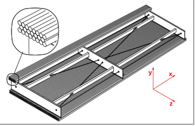
Figure 1 shows the layout of the MDT chambers which are built as an array of drift tubes and organized in two multilayers of 3 or 4 layers each.
y x
z
Figure 1: Sketch of a MDT chamber with indication of the local coordinate system.
The on-chamber front-end electronics consist of “mezzanine cards”, each of which handles signals from 24 MDT tubes. These cards have three 8-channel amplifier, shaper, discriminator (ASD) chips which feed one ATLAS MDT TDC (AMT) chip which digitizes time and charge measurements. De- pending on the chamber layout, 3 or 4 layer in a multilayer, the mezzanine handles 8 or 6 tubes per layer.
2.1 MDT data
The primary quantities are used in the calibration of MDT tubes are:
1. the drift timetT DCof the tube signal with respect to the bunch-crossing, measured by the TDC;
2. the charge collectedqADC, measured by the Wilkinson ADC;
3. the positionxalong the wire, measured by the trigger chamber system.
The Detector Control System (DCS) and the alignment system provide some other information relevant to the MDT response:
• gas parameters, such as pressure and composition;
• tube high voltage and current draw;
• local temperatureT and magnetic field~B;
• electronics parameters, such as TDC threshold and ADC settings;
• geometry parameters, such the displacements and deformations of the chambers.
2.2 Definition of calibration parameters
The track position within a MDT tube is determined from the function r(t)which relates the nominal drift time, t, to the impact parameter, r, of the track with respect to the wire centre. It is therefore necessary to modify the raw TDC value (tT DC), subtracting a tube dependent offset, hereafter calledt0 and correcting for the local variations of the drift parameters. The error to be associated with the impact parameterrresults from a resolution function which again depends onrand which is also computed by the calibration process.
MDT calibration must compute the following parameters which will be stored in the ATLAS Condi- tions Database for use by the reconstruction program:
• the time offsett0(measured time for a track which hits the sense wire)
• the mean valueq0, and width σq, of the ADC counts distribution for each channel, to be used in the computation of time slewing corrections (see 2.4);
• ther(t)relation of the relevant calibration region, for the nominal values of all the relevant param- eters (gas, temperature, magnetic field, etc.);
• the parametrization of the spatial resolutionσ(r), which is a function ofr.
2.3 Calibration model
The model adopted for the calibration of the MDT spectrometer divides the whole spectrometer (con- sisting of 1,108 chambers containing 339,000 tubes) into a number ofcalibration regions, each using a unique calibration parametrization. In order to limit the number of calibration regions and to keep the corresponding data collection and analysis to a manageable size, the data inside a region are corrected for local differences in environmental parameters and reduced to the same nominal drift conditions. Then, the space-timer(t)functions are computed with an iterative method.
Ideally, if all parameters were correctly measured and their influence on ther(t)function were com- pletely known, only one r(t)function would be sufficient for the entire MDT system, independent of
time. In reality, however, the corrections and environmental conditions are not known with sufficient precision. The size and number of the calibration regions is a trade-off between conflicting require- ments, such as the statistical and systematic errors, the time spent to collect the data, the time variation of ther(t)functions, the amount of data to be processed, the processing time and the amount of informa- tion to be stored in the database (disk space, access speed) that is accessed by the reconstruction program (computer memory).
The expected number of calibration regions ranges between 2,500 and 15,000. One important re- quirement for the calibration software (both for the calibration algorithms themselves and for the database and the calibration services of the reconstruction) is the ability to manage a variable number of calibration regions of different size. Currently the minimum size implemented for a calibration region corresponds to one multilayer. As a starting point, a single calibration region will not include more than one multi- layer, since different multilayers have different gas lines and may be affected by differences of the gas mixture. Smaller calibration regions could be implemented, if needed, in areas where large magnetic field gradients would result too difficult to correct, at the cost of some changes in the software framework.
2.4 Dependence upon external parameters
The time measured by the TDC,tT DC, needs to be corrected for various effects before it can be used as a drift time,tDri f t. Assuming that all the relevant parameters, as defined in section 2.1, are known, the procedure consists of the following steps:
1. The individual tube time offset,t0, is subtracted from the TDC valuetT DC (expressed in nanosec- onds):
t0=tT DC−t0 (1)
2. All the relevant corrections are applied, under the assumption that they are small enough to factor- ize:
tDri f t=t0+
∑
i
δti(t0) (2)
Some of the corrections are related to track/event -specific parameters, such as the hit position and signal amplitude:
• the time-of-flight correction, which takes into account the time elapsed between the LHC bunch crossing and the particle reaching the MDT.
• the trigger time correction, which accounts for the time difference between the bunch crossing clock and a trigger (relevant only to cosmic-ray triggered events).
• the propagation time correction, which accounts for the signal propagation in the MDT wire before reaching the front-end electronics, located on one end of the tube. The correction is based upon the second coordinate measurement provided by the trigger detectors.
• the time slewing correction, accounting for the variation of the threshold crossing time between signals with different amplitudes. The correction is based on the measured charge in the Wilkinson ADC.
All the other correctionsδti(temperature, magnetic field, cavern background, gas composition, wire sag) are instead due to the difference between the nominal values of these parametersa∗j, for which the r(t)relation is defined, and the measured values ¯aj:
δti=δti(t0,a∗j,a¯j)
effect size strategy references time slewing resolution degradation (≈40µm), negligible systematics correct [2–4]
temperature systematic variation of total drift timeδtmax/δT =−2.4ns/K correct [4–6]
magnetic field
(transverse to systematic variation of total drift timeδtmax/δB2=70ns/Tesla2 correct [7]
drift direction)
cavern background loss of efficiency and resolution degradation, negligible systematics neglect [8]
gas composition large systematic variations of total drift time calibrate [9]
wire sag systematic variations of total drift time (20 ns for 500µm sags) correct [10]
Table 1: List of corrections: columnreferencescontains the references to the literature for further details.
(e.g. the r(t) is defined for a nominal value T∗ of the temperature, while the measured value ¯T can be different). Some of these effects (e.g. the ~B dependence) should be stable in time, and induce a variation in the measured drift time as a function of the hit position along the tube, whereas others (e.g.
the temperature) may also vary with time and have to be carefully monitored. In the last case, a crucial part of the calibration procedure is the estimate of the time validity of the parameters (e.g. how often to access the temperature data).
Table 1 lists the non-trivial effects for which corrections have been studied and the strategy adopted.
Important features to be taken into account for the corrections are :
• they are universal, i.e. common to all the calibration regions;
• they must be measured and parametrized before the data taking, as a function of few time-dependent or event-dependent parameters;
• they must be applied consistently both in thet0and ther(t)computations;
• they must be applied consistently in the services used by the calibration, reconstruction and simu- lation software.
2.5 Computation of calibration parameters
2.5.1 Individual tube parameters
The first issue of the calibration procedure is to equalize the response of all the tubes in the same cali- bration region by removing different offsets.
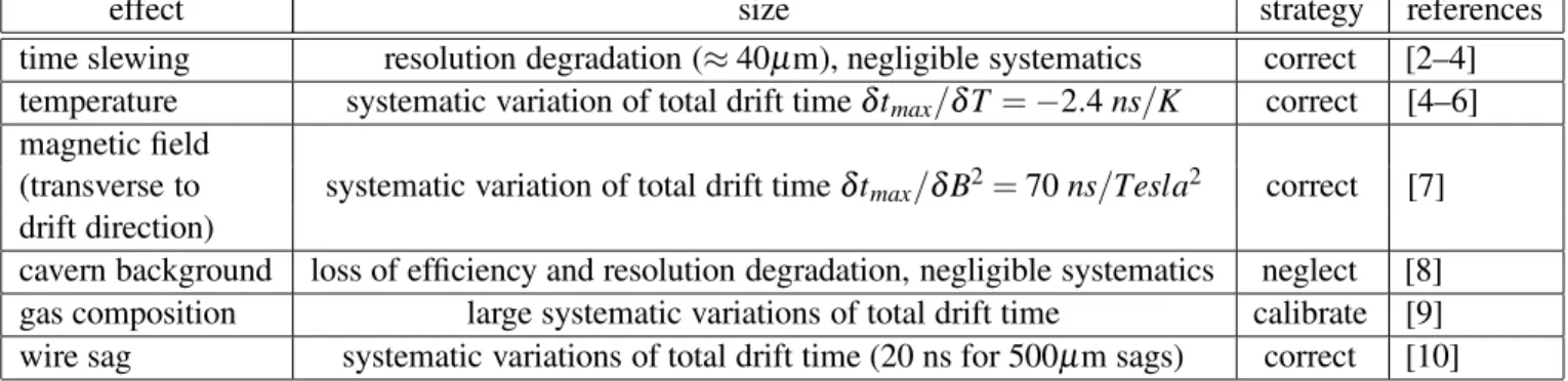
The measured drift time spectrum for each tube is obtained from the corrected timetDri f tof equation (2). A preliminary approximatet0is assumed in the computation of the correction functions δti. From the drift time spectrum two parameters, the “start” time, which can be identified with the t0 and the
“maximum drift time”, tmax can be extracted. An example of this distribution is shown in Figure 2 indicating t0 and tmax . Qualitatively, tracks with drift times ∼t0 pass near the wire, while drift times
∼(t0 +tmax) are caused by tracks passing near the tube wall. Parameters extracted from this distribution can also be used for monitoring purposes, as discussed in section 4.7.
The parametert0, computed after application of all timing corrections, accounts for the difference in cable length and electronics among different tubes of the same calibration region and for the mean value of the timing corrections.
The required accuracy is determined by its influence on the determination of ther(t)function. For an average drift velocityvdri f t ≈25µm/nsa maximum uncertaintyσ(r)≈20µm is achieved for∆t≈
measured time (ns) Events / 0.78 ns
tmax t0
Figure 2: A measured time spectrum with an arbitrary offset. The arrows indicate thet0andtmaxvalues.
The 8 parameter fit explained in the text is superimposed.
0.8ns. In thet0determination the relevant quantity is the relative time offset between tubes in the same calibration region. Small common offsets with respect to other regions are absorbed in ther(t)relation.
The parameter tmax is defined as the maximum drift time, i.e. after subtracting the t0 value (see Figure 2). Its value is used to monitor the tube performance, since it is very sensitive to all the gas, environment and electronics parameters. The value of tmax is not used directly in the reconstruction.
However, it can be used as a parameter in the functionsδti(e.g. to determine the wire sag and to correct ther(t)relation for the wire sag).
In test beam studies, several methods have been used to measuret0andtmax: 1. a global fit to the distribution, for example with the function [6]:
dN
dt =P1+
P2
1+P3exp
P5−t P4
h1+exp
P5−t P7
i
·h
1+exp
t−P6 P8
i, (3) wherePiare fitting parameters. In this procedure, sometimes the parametersP7andP8are fixed in the fit to speed up the convergence. The fit results are the parameterP5≡t0andP6≡t0 +tmax. 2. local fits to the same distribution in the regions neart0and (t0 +tmax) respectively.
3. method (1) or (2), followed by a redefinition of the value of t0 e.g. 5% or 10% of the full height (obtained subtracting a constant times the slope of the curve neart0) instead of 50% as in equation (3). The adoption of this recipe, which is compensated by an automatic variation in the r(t)relation, moves all the gas and environment dependence into ther(t)and leads to more stable values oft0[11,12].
It must be noted that the data shown in Figure 2 have been taken in a test beam in the absence of significant background, with a beam spot of a few centimeters. However, the requirement of a match with the trigger road (see Section 3) reduces the background significantly and should allow a reliable determination of the above parameters even in the presence of backgrounds up to five times the nominal level.
2.6 Calibration region parameters
2.6.1 The r(t) relation
The calibration procedure (autocalibration) uses the data themselves to determine ther(t)relation. The procedure is based on an iterative fit that requires several thousand muon tracks. The r(t) relation is modified until the quality of the track fit is satisfactory. The details of the algorithms are summarized in Section 2.6.2 and discussed in the bibliography.
The autocalibration has to be applied to a region of the spectrometer with MDTs operated under similar environmental conditions (gas, temperature, B field, ...), i.e. to a single calibration region, as discussed in Section 2. The autocalibration algorithms require the corrected drift times (tDri f t, as defined in Section 2.4).
Several autocalibration algorithms have been developed. The modular calibration software allows configuration of multiple correction algorithms and varied parametrizations the data, while utilizing a common definition of the calibration regions and a well-defined interface between the calibration frame- work and the algorithm.
In general, independent of the algorithm used, autocalibration needs a distribution of tracks over a wide range of angles. It has been shown (see the references in Section 2.6.2) that with a sample of parallel tracks is not possible to extract a unique physical r(t). This requirement has an influence on the minimum size in η of a calibration region. Also the uniformity of the track sample over the area of the calibration region is an essential requirement to minimize the systematic error. A few regions of the spectrometer require more care in the calibrations, e.g. where the variation of the magnetic field is larger (BIS chambers) or for chambers atθ ∼30◦, where tracks produce nearly equal drift radii in all the layers.
2.6.2 The calibration methods
Two different algorithms have been developed and integrated in the software framework:
• In the original method [13], the entire time spectrum is divided in bins with a typical size of 1/50 of the maximum drift time. Then, the averages (ti,ri) are either taken from a previous calibration or computed for each time bin from the integration of the time distribution of Figure 2. A linear interpolation between the points provides the radial distance from the wire of each measured time.
Using these radii to form drift circles, the best tangent line to the tube hits is determined by a fitting procedure, assuming a preliminary resolution functionσ(r). For each time bin the average of the signed residuals is then evaluated and the corresponding value of the drift radius ri is modified accordingly. The process is iterated until the average of the corrections is smaller than the required accuracy of better than 20µm. In test beam studies, with a sample of 10,000 tracks, i.e. an average number of 200 tracks for each time bin, and assuming (conservatively) a r.m.s. of the residuals of 100µm, an accuracy of about 10µm in ther(t)relation is achieved.
• The analytic autocalibration or matrix method [8,14] is an improved autocalibration method, based on a matrix formalism. It was designed to take optimum advantage of all available information.
The initial relationship rinitial(t), does not need to be very accurate, 0.5mm precision is enough to reconstruct straight track segments in the MDT chambers. If therinitial(t)is altered by a small quantityδ(t), the residual∆kof thekth hit changes by
δ(∆k) =
∑
l
∂
∂l
∆k·δ(tl) =
∑
l
Mklδ(tl). (4)
The correction δ(t) to the initial rinitial(t) is parametrized as a linear combination of base func- tions, for instance Legendre polynomials. The coefficients of the base functions are determined by minimizing
χ2=
∑
segments
∑
hits k
[∆k−∑lMklδ(tl)]2
σ2(∆k) . (5)
The coefficients of the matrix (Mkl) can be calculated analytically andδ(t) is given as a linear combination of base functions: the χ2minimization can be solved analytically, hence the name
“analytic autocalibration method”. Monte-Carlo and test-beam studies show that δ(t)is almost the correct correction function, i.e.δ(t)is close torinitial(t)−rtrue(t). However to obtainr(t)with the required accuracy of 20µm, the method has to be applied iteratively. It converges toδ(t) =0 after typically 5 iterations.
2.6.3 The resolution,σ(r)
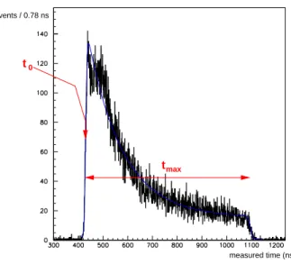
Figure 3: The resolutionσ(r)as a function ofrfor several values of the background rate [8].
The resolution function, σ(r), is also required by the reconstruction programs. The dependence of σ(r)as a function ofris shown in Figure 3 from reference [8] both in absence and in presence of high background rates. All the methods which compute the r(t)relation measure σ(r) as a by-product by adjusting it in comparison with the distribution of the residuals and theχ2probability of the track fit.
Autocalibration and resolution estimation use simple track fit algorithms, either linear over one mul- tilayer or parabolic over two multilayers. The choice between the two options will be based upon perfor- mance achieved in the experiment and may differ in different regions.
2.7 Required statistics
Several studies have investigated the amount of data necessary to fit the parameters discussed here with the desired statistical error [8,12,15,16]. The main conclusions are that:
• for ther(t)function the minimum statistics slightly depends on the algorithm adopted. We assume here that a minimum of 10,000 segments is needed per calibration region. Accounting for the
number of regions crossed by a track (3 chamber stations, i.e. 6 multilayers) and assuming 2,500 to 15,000 regions, (4 to 25)×106good muon tracks are required for the whole spectrometer;
• fort0andtmaxthe dependence of the statistical error on the the total number (Nhits) of entries in the histogram can be parametrized as
∆t0'90 ns/p
Nhits; ∆tmax'200 ns/p
Nhits. (6)
Therefore, about 10,000 good hits per spectrum would be needed to reach a precision of 1 ns on t0. Since a single muon crosses at least 20 tubes, roughly∼2×10⁸good muon tracks are required for single tube t0 computation in the whole spectrometer. Howevert0 differences among the 24 tubes connected to the same front-end mezzanine card are≈ 1 ns and are systematic and stable in time, allowing a reduction of the minimum statistics for the measurement of this parameter. The reduction factor is 6 or 8, depending on the chamber layer layout. 30×106tracks would allow to measure the single tubetmaxwith a resolution of 5 ns.
3 Muon calibration stream
It should be noted that the expected maximum rate of muon triggered events on tape is 40 Hz. In order to achieve enough statistics to be able to follow the possible time variations of the MDT calibrations a dedicated procedure, allowing the extraction of muon triggered events at a higher rate. We aim at collecting enough statistics to allow a calibration per day with a sample of ≈30×106 muon tracks.
Accounting for data taking efficiency we require an acquisition rate of≈1kHz. This section is devoted to the description of the adopted solution, detailed in reference [17].
Extracting data online from the ATLAS trigger/DAQ system makes additional requirements on the extraction system. It must not affect regular data taking, add any latency to the trigger, or introduce error conditions in case of failure. These requirements can be summarized as follows:
• The data collection scheme must fit in the current trigger/DAQ architecture.
• The data fragments must contain only the data relevant for calibrations.
• The overhead of tasks providing calibration data collection must be negligible.
• The required bandwidth must be already available in the trigger/DAQ system.
• Some flexibility is desirable in order to provide data streaming, data pre-selection based upon the pT of the candidate track and seeding of the pattern recognition used by the calibration.
3.1 MDT chambers readout architecture
MDT chambers are read out by on-chamber ADCs and TDCs [18]; data are then fed into the CSM (Chamber Service Module) [19] . Each set of 6 CSMs, i.e. 6 chambers, is connected via optical links to one Muon Read-Out Driver (MROD) [20].
The first level trigger (level-1) selects high momentum muon candidates. Starting from the hits in the trigger chambers, it identifies a Region of Interest (RoI), defined as a trigger tower as shown in Figure 4 plus the closest tower, inη, to the level-1 hit pattern. The RoI is then used to input the second-level trigger (level-2) with data from trigger and precision chambers to perform local data reconstruction. It is then natural to organize the detector readout into trigger towers as shown in the figure.
Each MROD receives data from the 6 chambers in a trigger tower. Only data from a RoI (i.e. two MRODs) are transferred to the level-2 trigger, thus minimizing the data throughput from the DAQ system
Figure 4: Data readout organization for the muon barrel.
to the level-2 trigger. The fragments of accepted events are then collected by ReadOut Systems (ROS) [21] and sent to an event-building farm node (Sub Farm Input, SFI). The full events are then analyzed by the event filter and sent to a SFO (Sub Farm Output) process to be staged on disk [22].
3.2 Muon calibration stream data sources
In principle, data can be extracted at any level using foreseen data sampling and monitoring facilities [23].
However there are the following drawbacks:
• the required rate is not achievable after the level-2 trigger, whose overall output rate is of the order of 1 kHz;
• the MROD rate is high (75 to 100 kHz), but there is no knowledge of the RoI, nor of RPC and TGC hits, and a complete event building at the required rate would be needed.
At level-2, the input muon rate is about 12 kHz (for low luminosity and 6 GeV/c pT threshold) and only data from the RoI are moved. In addition, the muon trigger algorithm run at level-2 deals only with data related to the candidate muon track. Since this algorithm reconstructs the track, the level-2 trigger is the ideal place to extract muon data, selecting hits in the track and adding the fit parameters in order to seed the calibration procedures to allow fast convergence.
3.3 Level-2 calibration stream
The level-2 trigger algorithms run on PCs interconnected by a network to exchange event data. The level- 2 muon trigger task,µFast [24], confirms the muons found at level-1 by a more precise muon momentum measurement and rejects fake level-1 triggers induced by physics background. The overall latency of the level-2 trigger system imposes an upper limit of≈10 ms to the execution time of this algorithm, which includes the access to the data and their decoding. µFast processes the data in three sequential steps:
1. pattern recognition involving trigger chamber hits and the position of the MDT hit tubes, 2. a track fit performed on each MDT chamber,
3. apT estimate using look-up-tables (LUTs) in order to avoid time-consuming fitting methods.
The track position at the entrance of the spectrometer, the direction of flight and the pT at the interaction vertex are computed. At this stage, the interaction vertex is defined by the average position of the interactions provided by offline measurements.
The pattern recognition is designed to select clusters of MDT tubes belonging to a muon track without using the drift time measurement. Being seeded by the level-1 trigger data, muon roads are opened in each MDT chamber and hit tubes are collected according to the position of the sensitive wire. The road width is tuned to collect 96% of muon hits. The typical size of a road is 20 cm.
The muon calibration stream consists of pseudo-events, one for each muon track candidate, collecting both the trigger chamber data accessed byµFast and the MDT hits within the level-2 pattern recognition road. The pseudo-event header also includes the estimated pT and the direction of flight.
A first evaluation of the extracted data size is about 800 bytes per pseudo-event. Data extracted from the level-2 nodes can then be concentrated in a calibration server and made available to be distributed to calibration farms. Data concentration can happen in one or two steps, either directly sending data from the level-2 nodes to the calibration server or sending data to the local file/boot servers in the level- 2 racks [25] and, in a second step, to the calibration server. The first option avoids using local server resources, and the second improves the flexibility of the system and allows optimized use of the network.
The second option was chosen for the extraction of the muon calibration stream.
3.4 Implementation
The general system architecture of the calibration stream is shown in Figure 5. The level-2 trigger algorithms run in a farm of about 500 processors, divided in 20 racks. 25 nodes in a rack are booted from a local disk/file server. Each node runs a level-2 Processing Unit (L2PU) on each of its CPU cores.
Gatherer Gatherer
disk
x 25 x 25
x x ~~2020
~ 9.6 MB/s~ 9.6 MB/s
~ 480 ~ 480 kB/skB/s
~ ~ 480 480 kB/skB/s
Figure 5: Data extraction and distribution architecture.
Data prepared in L2PU are sent to a collector in the local file server, grouped in multi-event packets and sent to a global collector, which writes them to disk. The throughput to each local server is about 480 kB/s and the global throughput is about 9.6 MB/s. Collected data can then be sent to calibration farms for processing. In the proposed architecture, final data destination can be easily decided on the basis of the calibration region allowing different CPUs and different farms to work independently on different calibration regions. In order to fulfill the requirements, the latency added to the muon level- 2 trigger must be negligible with respect to the processing time (<10 ms), the load on local servers must be negligible and data distribution channels to the farms on the WAN must sustain the data rate.
Results of the extensive tests performed to validate the muon calibration stream extraction are presented in Section 5.1.
4 Muon calibration processing
As discussed in Section 2.7, a total of 30×106tracks has to be processed for a typical LHC data-taking day. Moreover, the proposed organization of the ATLAS production requires fast (1 day) availability of the calibration constants which are to be used by the reconstruction software. Assuming the present speed of the calibration programme, including data decoding and database access, and the present performance of the computing facilities, these requirements correspond to the availability of few hundred processors, with high reliability. In addition, the production of the constants needs the dedicated effort of detector and analysis experts, especially during the commissioning and the first data taking periods.
We have chosen a solution, which appears to be the best compromise between efficiency, reliability
and optimal use of computing facilities. The muon groups of Ann Arbor1), MPI Munich2), LMU3), Roma “La Sapienza”4) and Roma Tre5) have established in Ann Arbor1), Munich2,3) and Roma “La Sapienza”4)threeCalibration Centers. These farms, which are Tier2s in the ATLAS computing system, have been equipped with the software packages required by the computation (see Section 4.2) and have agreed to give high priority to the computation of the calibration constants during data taking periods.
Each Calibration Centre will perform a fraction of the total computation, with small overlaps for testing and checking purposes. To ensure the necessary redundancy, the Calibration Centres will run the same software and are ready to back up each other in case of failures of the local systems or of the data transmission. In such a case, a larger number of processors will be allocated to the calibration task, to maintain the overall speed.
The computation model foresees that the data are sent to the Calibration Centres synchronously, in blocks of few GB as soon as they are available from the calibration stream. Therefore the local computation (and the data quality check) starts almost immediately after the beginning of the data taking.
Only the second part of the computation (the iterative fit, see section 4.5), which is much faster than the real processing of all the tracks, is performed at the end of the data taking.
At the end of the computation, the results (i.e. the constants, together with the assessment of the quality of the data) are sent back to the central computing facilities at CERN, checked for overlaps, merged and inserted in the ATLAS main reconstruction database.
4.1 Muon Calibration data flow
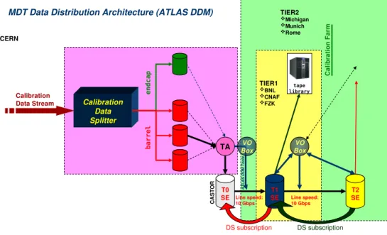
The data in the calibration stream are transferred to the local Calibration Centres using the ATLAS Distributed Data Management (DDM). This process consists of few steps, detailed in Figure 6. The data, as soon as they are created, are split in files approximately 1 GByte each by the local Calibration Data Splitter (a program belonging to the ATLAS DAQ). The files are registered in the Grid Storage Elements at the CERN Tier0 (in future this step could be skipped in case of a dedicated link to Tier1s) and transferred to the Grid Storage Elements. A calibration dataset (i.e. a group of files accessible to users) is created by the Transfer Agent (the Grid program which takes care of data transmission) for each calibration session, typically corresponding to an LHC fill.
The Transfer Agent subscribes the calibration datasets to both Tier1 and Tier2 Storage Elements.
The subscribed datasets are automatically transferred by the DDM from the Tier0 to the appropriate Tier1 (in Germany, Italy and United States for Munich, Roma and Michigan respectively) and then to the Tier2. This operation is performed in quasi-streaming mode via the FTS (File Transfer Service) channel [26, 27]. In future the transfer priority will be managed by the DDM Quality of Services (QoS) assured by the Centres/resource owners.
The network bandwidth required by the calibration process amounts roughly to 100 GByte/day (data transfer CERN→Tier2s) and 50 MByte/day (calibration constants transfer Tier2s→CERN database).
While the second requirement is easily fulfilled by the existing facilities, the first requires an appropriate network bandwidth corresponding to the maximum possible volume of data (all data in all the centres) and to the maximum level-2 throughput (9.6 MB/s).
To check the feasibility of remote calibration, the data transfer rate between Tier0 and the Italian Tier1 Centre at CNAF has been measured. Though QoS is not yet implemented, and data compression was not used, the measured data transfer rate was always higher than the maximum required.
1)The University of Michigan, Ann Arbor, USA
2)Max-Planck-Institut f¨ur Physik, M¨unchen, Germany
3)Fakult¨at f¨ur Physik der Ludwig-Maximilians-Universit¨at M¨unchen, Garching, Germany
4)INFN Roma and Universit`a La Sapienza, Dipartimento di Fisica, Italy
5)INFN Roma Tre and Universit`a di Roma Tre, Dipartimento di Fisica, Roma, Italy
Figure 6: The muon calibration stream data transfer using the ATLAS Distributed Data Management.
The Tier1 will be responsible of backing up the data, using CASTOR or similar systems as a target storage element.
The Calibration Farms in the Tier2 will be able to process the files as they will be available in the local Storage elements. Files belonging to an incomplete dataset may be used as soon as they are transferred.
4.2 Architecture of a Calibration Tier2 Centre
The Calibration Tier2 have the same components as a standard ATLAS Tier2 [28] with additional job and data management components to control the calibration activity. These components allow for ad- ditional services, such as different partitioning and allocation of the resources, the dynamic partitioning of the computing resources for the calibration tasks and the partitioning and reservation of the storage resources for the calibration tasks. A dedicated database (in the present implementation the ORACLE (TM) database) and some network QoS are also required.
The Job Management components include, in addition to the standard Tier2 components, entry points for Grid jobs which need ahost certificateto operate, and are integrated in a Batch Queue manager. Some of the Tier2 worker nodes (presently about one third of the processors) are dedicated to the calibration activity.
The storage management requires the support of the GSIFTP transfer protocol, the access to CAS- TOR, DPM and dCache [26, 27]. All the current Centres already have or plan to have these facili- ties (EGEE SRM SEs in Rome and Munich, supporting DQ2, OSG SE in Michigan, supporting DQ2 (GSIFTP) through the UltraLight network facility [26, 27]). The storage space in local Tier2, dedicated for calibration tasks amounts to about 1 TB of disk space. As mentioned above, the ORACLE database is used to store the final calibration constants and to maintain the bookkeeping of the operations.
During the ATLAS data-taking periods, the nodes performing calibration tasks should be mainly dedicated to this activity and excluded from Grid access, although they should be instrumented with all the Grid facilities to access the data. This could be done by creating a separate partition within the Tier2 infrastructure and reconfiguring the underlying Batch Queue system by adding a calibration queue/share (”static” reservation of working nodes). Although this method is not very efficient, it guarantees the
required performance. In future a more sophisticated system will be implemented, based on dynamical farm partitioning and shares (guaranteed share of resources, reserved for calibration purposes, plus a pool of additional resources with higher priority for calibration tasks).
When the resources from the pool are not needed, they may be used for normal Tier2 tasks (mainly simulation and analysis). No check-pointing is currently possible, which means that it is not possible to temporarily suspend a job giving priority to another one, thus the higher priority for the calibration tasks can only be used at the scheduling level.
In addition, a dedicated node in the Tier2 will be dedicated to calibration data preparation and cleanup (see next section) as a Local Calibration Data Splitter.
4.3 Data Processing
The local Calibration Data Splitter permanently watches for incoming data. As soon as the first data arrive, this node starts its operations, splitting the input data files in separate output streams according to a predefined scheme (e.g. different angular regions of the ATLAS muon spectrometer) and submitting a job to the calibration batch queue. This allows for the creation of the output ROOT files [29] (see section 4.4) in parallel.
Partial checks of the data integrity and quality are performed as soon as the data are available, to allow for fast recognition of possible hardware or DAQ failures on the high statistics sample of the calibration stream.
When sufficient data have been processed, or at the end of data-taking, either a local operator or an automatic procedure starts the final phase of data processing, which includes the checks of the data quality and calculation of the calibration constants (see section 4.5).
The monitoring of the calibration is performed by a monitoring client, integrated in the calibration application and in the splitter agent. The calibration status of each Centre will be published in a central server visible to the full ATLAS collaboration. The calibration stream data could be accessed directly from the local storage in the Tier2s, e.g. directly from ROOT usingGFAL(RFIO, dcap, ... [26,27]). Data can be either directly accessed from the Storage Elements or copied locally and then analyzed either by the calibration application or by the local Calibration Data Splitter.
At the end of the calibration, when all the relevant data have been properly stored, the operators should tag a calibration asdone. Then, the data could be in principle released (unsubscribed), and deleted from the Tier2 storage (at the moment this process is manual). In case there is a need of reprocessing, the data have to be re-subscribed from the Tier1, although a manual option exists to keep the data for a longer period in the Tier2 storage. A ”garbage collection” process will also be provided, to put a limit on the maximum amount of local Tier2 storage that can be used for calibration data.
If one of the calibration Tier2 is temporary unable to process the data, another Centre will take over its responsibility of data processing. When this case is announced by the local crew, the CERN calibration data splitter is manually reconfigured and restarted to redirect the data to the proper place, until the problems are fixed. This operation requires only a single parameter change in the configuration files.
4.4 Production of calibration data
The starting point for the production of calibration data are the data streams already split into angular regions, each one containing a limited number of calibration regions. Each stream contains both MDT and trigger chamber data. As soon as a stream is available on a dedicated area of the disk pool of the Tier2, a reconstruction job is run to produce a ROOT Tree with all the required information needed in the subsequent steps. The reconstruction job runs in the ATHENA framework and fits track segments in the calibration regions [30]. Starting from a bundle of hits already selected by the level-2 trigger algorithm,
the package performs pattern recognition and track fit and outputs information on fitted segments and associated hits. In order to produce segments efficiently and so as not to introduce any bias, reasonable values of the calibration constants are used (typically those computed for the same region in a previous calibration job). The list of the variables stored in the Tree includes the parameters of the fitted segments and their position in space, the χ2 of the fit, a quality factor, the drift time, radius and ADC value for all the hits in the segment as well as all the corrections applied to the drift time by the reconstruction program.
4.5 Measurement of calibration parameters
The ROOT files containing the Tree with the segments are analyzed within the ATHENA framework.
Each calibration step (e.g. t0 fit, r(t) calibration, resolution determination) is done by a separate run of ATHENA. An ATHENA Algorithm (CalibNtupleAnalysisAlg) takes care of reading the Tree and preparing the data for the calibration algorithms which are implemented as ATHENA Tools (calibration tools). An ATHENA Service reads in the results from the previous calibration steps and sends them to the CalibNtupleAnalysisAlg and the calibration tools. Another service collects the results from the calibration tools and takes care of writing out the results.
The CalibNtupleAnalysisAlg selects, from the Tree of a given angular region, the segments which pass through the requested calibration region. For each event only one segment per calibration region is selected, the one which has the most MDT hits. If there are two segments with the same number of hits the one with the highest fit-probability is selected.
For this segment the calibration corrections which were used in the reconstruction are inverted, so that the calibration results are absolute. In particular the t0 which was used in the reconstruction and saved in the Tree is added to the drift time. The results from the previous calibration steps are then applied to the hits in the segments. These segments are then passed to the calibration tools.
The results are collected by the MdtCalibDbOutputSvc, which is an ATHENA service. The results are checked to make sure the number of producedt0values matches the number of tubes in the chamber and results formatted. At finalization, the service can write out the calibration results in different formats (ASCII files, a ROOT-based database, and the Calibration Database described in Section 4.6). The ASCII files are read in by the input service for the next calibration steps.
4.6 Databases
The quality and stability of the individual tube parameters, as well as of the r(t)relation, must be con- tinuously monitored. In addition to the limited number of calibration parameters to be used by the reconstruction, the processing described in previous sections produces a sizable amount of information ( 50 MB/day) essential to evaluate the quality of the calibrations.
A dedicated MDT database (Calibration Database) [31] is thus being implemented to store the com- plete calibration information. Validation procedures will make use of the additional information, as described in Section 4.7, to ensure that the calibration constants have been correctly computed. Also, the newly produced constants will be compared to those from the previous data taking to decide whether the Conditions Database must be updated. The full information produced at every stage will be stored in local ORACLE Calibration Databases that will be replicated via ORACLE streams to a central database located at CERN. This procedure will allow each Calibration Centre to access the data produced by the others and to eventually provide back-up should one site become unavailable for any reason.
The validated calibration constants will be extracted from the CERN Calibration Database and stored into the ATLAS Conditions Database for subsequent use in reconstruction and data analysis. This data management model has the major advantage that the Calibration Database is completely decoupled from
the clients of the calibration and thus it can be modified without affecting the reconstruction; more- over, while the Conditions Database is optimized for reconstruction access, the Calibration Database is optimized for access by calibration and validation programs.
Calibration Centres will need to use the Conditions Database to access the conditions data that are relevant for the calculation of MDT calibrations such as: alignment constants from the Muon Spec- trometer optical alignment system, magnetic field and temperature maps, data quality information. Since Calibration Centres are Tier2 Sites, the Conditions Database is available through the standard distribution channel (SQLite files). However it is not possible to be notified in real-time of changes in the Conditions Database tables that are relevant for the calibration through this channel. For this reason, the Calibration Centres will maintain an ORACLE replica of the needed tables of Conditions Database. This replica will be kept up-to-date using the ORACLE streams mechanism which automatically pushes data from the Tier0 to the Tier2 whenever the tables are updated.
Some replication tests of tube calibration constants between Calibration Centres and CERN have already been successfully performed. No issues of latency or bandwidth are expected for the standard operation because of the small amount of data that will be replicated.
4.7 Validation of calibration parameters
The validation and monitoring of the MDT calibration parameters are important parts of the data quality assessment for the muon system. The validation procedures at the Calibration Centres are based on the experience with cosmic rays at test facilities [32], during ATLAS commissioning, as well as in muon test beams at CERN [6,33].
Data quality assessment for the MDT calibration constants is divided into two subjects : - Definition of acceptance criteria and validation status flagging;
- Monitoring of time stability and checking for smooth or sudden changes in operating conditions.
In the first case the process results in the validation of calibration constants for individual tubes (from drift time distribution analysis) or calibration regions (fromr(t)relation validation).
In the second case, observed variations of the calibration constants, allow detecting possible effects such as:
- sudden changes induced by the front end electronics initialization procedures;
- variation of uncorrelated noise (e.g. variations of the number of hits outside the physical region);
- variations in the gas composition or purity (e.g. changes in the maximum drift time);
- variations in resolution (e.g. changes in the rise-time parameter).
The implementation of the validation process is based (and only depends) on the calibration parame- ters read in from the Calibration Database. It is essentially based on the analysis of the fit to single tubes drift time distributions and of ther(t)relation obtained in the calibration regions.
If the minimal statistics required for meaningful fits is not reached (see section 2.7), drift time spectra will be produced for the tubes readout by the same mezzanine card. In this case the same constants are assigned to all the tubes in the same group.
Quality criteria are based on limits defined for those parameters expected to be reasonably stable in time and directly linked to the characteristics of the response of the drift tubes [12]. Limits are established either from the previous values assumed by the parameters or from the average behavior of all the tubes in a chamber. The quality of the fit is monitored by theχ2value. Unacceptable values of the fit parameters
TCP(C++) TCP(Python) Monitor
Sender <1% <1% <1%
Local server 1% 6% 2%
Final server 4% 14% 6%
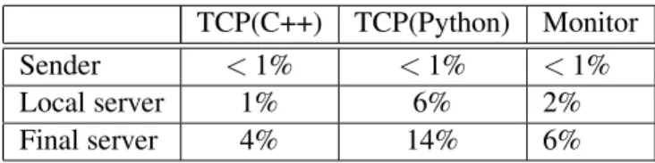
Table 2: CPU usage
can be due to failures of either the hardware or electronics of the MDTs. Outliers tubes are flagged with abadstatus in the Calibration Database. For these tubes, the first action is to inspect time distributions and results of the various steps of the fit. The next step is to report the diagnosis to hardware experts and to the Data Quality group for further detailed studies. Malfunctioning tubes are eventually flagged in the Conditions Database.
Quality criteria on ther(t)relations are mainly based on the definition of a quality parameter account- ing for their properties of smoothness and monotonicity and on the analysis of the residuals distribution.
Ther(t)functions are then compared to the ones from previous calibrations and the Conditions Database is updated in presence of significant changes.
5 MDT calibration Test results
5.1 Tests of muon calibration stream extraction
The data extraction procedure has been tested on the ATLAS TDAQ pre-series [34] to verify that the CPU load added by the muon calibration stream is negligible both on the level-2 processors and on the local servers. The level-2 trigger is decoupled from the rest of the system by ring buffers: each L2PU writes the muon stream data to a ring buffer, a reader collects data from the buffers in the node and sends them to a data collector. If the buffer is full the event is discarded and the L2PU starts processing the next event. In this way, the only latency added to the trigger is due to data preparation (less than 200µs) and no effect is due to back-pressure (if any) of the data extraction system. The only other relevant parameter to be measured in the level-2 nodes is the fraction of CPU time used by the data sender. In our test, a data producer emulates the behavior of the L2PUs in 25 bi-processor nodes in a rack; each node runs three emulators injecting fake data packets to the ring buffer at the expected rate.
Local server’s resources, both in terms of I/O and in terms of CPU usage, must be dedicated to server specific tasks like NFS service, boot service, DAQ specific services and controllers. It is therefore essential to measure also the additional CPU load on the local server. On the other hand, NFS service is not CPU intensive and the needed throughput for data extraction is negligible with respect to the available bandwidth.
Several protocols have been used to build client and server applications, In all the cases, the same application is used as local and final calibration server; the local server packs data in 64 kB packets before sending them to the final server.
The measurements have been performed in two phases. In the first one, the data producers and the buffer readers running on the level-2 nodes sent data to a calibration server running on the local file server. This calibration server packed data, and sent them to another server running on another rack of the pre-series. The measurements on the final server have been performed using the data producer to emulate the output of the local server and the buffer reader to send data to the final server. Using 20 nodes in a rack, we emulated the same number of local servers connected to the final calibration server. Table 2 shows the CPU usage for TCP based applications written in C++ and in Python and for applications built on top of the Atlas online monitoring library (based on Common Object Request Broker Architecture).
sample event size number of events processing time number of hits
on segment in sector 5
no stream 18KB 80K 660 ms/event 1.3M
(muon spectrometer only)
stream 0.5KB 43K 270 ms/pseudo-event 0.5M
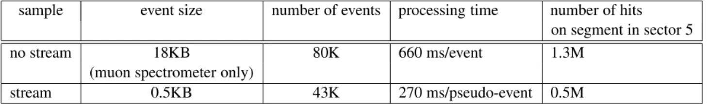
Table 3: Comparison between standard data and muon calibration stream in the same cosmic-ray run.
5.2 Data challenge with simulated data
The Calibration Centres in Ann Arbor and in Rome have produced muon calibration stream files from a sample of simulated single muons µFast level-2 algorithm (barrel only). The local Calibration Data Splitter, configured with a small number of calibration regions, was used to split the muon calibration stream files as they became available and to submit the jobs for production of the ROOT Trees. 1.3M and 1.5M events have been successfully processed at Rome and Michigan, respectively.
5.3 Calibration of commissioning data
µFast level-2 barrel algorithm in offline mode, followed by the ROOT Tree production, was also run on a subsample of the cosmic data taken during the detector commissioning, with RPC trigger active only in sector 5. Cross-checking with the ROOT Tree directly produced on the standard data, it was possible to
1. validate the decoding of the MDT and RPC data fragments;
2. validate the hit selection performed byµFast;
3. compare the calibration constants computed on streamed and on standard data;
4. measure the processing time per pseudo-event.
Table 3 compares event size, number of events, processing time per event and number of hits in sector 5 associated to segments between standard data and muon calibration stream.
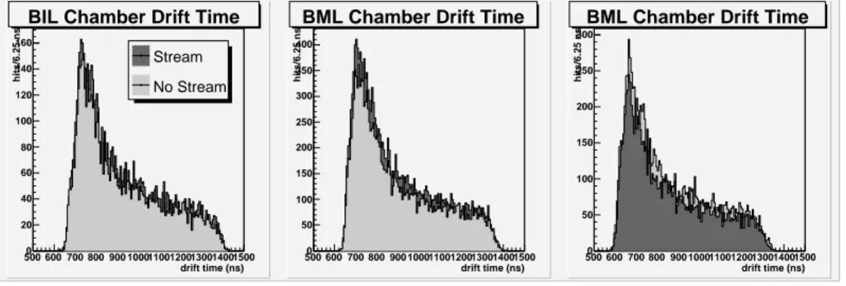
The muon calibration stream data size and processing time are smaller, but also the number of hits is reduced with respect to standard data. However the segments used within the calibration are selected by additional criteria (see Section 4.4). Figure 7 shows that despite the large difference in the number of hits, the statistics actually used by the calibration after the selection of the best segments are comparable.
In conclusion, the muon calibration stream reduces significantly the data size and the processing time, without affecting the statistics available for the calibration.
6 Conclusion
This paper describes the calibration procedures for the Monitored Drift Tube detectors of the ATLAS Muon Spectrometer, their implementation and early tests. In order to match the mechanical and intrinsic accuracy of the detector, calibration constants which provide 20µm tracking precision are required. The model described in this paper considers the extraction of 1 kHz single muon data directly from the Level-2 trigger processors. A dedicated processing architecture, based on externalCalibration Centres at ATLAS Tier2s, will be used to produce calibrations for collision data, perform validations, and provide them to reconstruction within one day from the end of the LHC fill. The implementation of this scheme
bil33stream Entries 6846 Mean 923.2 RMS 194.6
drift time (ns) 500 600 700 800 900 100011001200130014001500
hits/6.25 ns
0 20 40 60 80 100 120 140 160
bil33stream Entries 6846 Mean 923.2 RMS 194.6
BIL Chamber Drift Time
Stream No Stream
bml33stream Entries 17821 Mean 901.1 RMS 194.1
drift time (ns) 500 600 700 800 900 100011001200130014001500
hits/6.25 ns
0 50 100 150 200 250 300 350 400
bml33stream Entries 17821 Mean 901.1 RMS 194.1
BML Chamber Drift Time
bol33nostream Entries 11231 Mean 859.2 RMS 194.4
drift time (ns) 500 600 700 800 900 100011001200130014001500
hits/6.25 ns
0 50 100 150 200 250 300
bol33nostream Entries 11231 Mean 859.2 RMS 194.4
BML Chamber Drift Time
Figure 7: Drift time spectra for a BIL, a BML and a BOL chamber in run 20304 (cosmic-run M4, September 2007) obtained from standard data and from the muon calibration stream. In BIL and BML the cleaner muon calibration stream allows to retain few more hits for the calibration. Conversely BOL chamber sees many non-pointing cosmic rays which are rejected by the trigger selection and more hits are retained in standard data.
is well advanced and the method is being commissioned “in situ” together with the Muon Spectrometer with cosmic-ray runs.
References
[1] ATLAS Collaboration, The Atlas Experiment at the CERN Large Hadron Collider, submitted to Journal of Instrumentation (2007).
[2] Deile, M. et al., Resolution and efficiency of the ATLAS muon drift-tube chambers at high back- ground rates, Nucl. Instrum. Meth.A535(2004) 212–215.
[3] Bagnaia, P. et al., Charge-dependent corrections to the time response of ATLAS muon chambers, Nucl. Instrum. Meth.A533(2004) 344–352.
[4] Branchini, P. et al., Study of the drift properties of high-pressure drift tubes for the ATLAS muon spectrometer, IEEE Trans. Nucl. Sci.53(2006) 317–321.
[5] Baroncelli, T. et al., Study of temperature and gas composition effects in rt relations of ATLAS MDT BIL Chambers, ATLAS Note ATL-MUON-2004-018, CERN, Geneva, Jul 2004.
[6] Avolio, G. et al., Test of the first BIL tracking chamber for the ATLAS muon spectrometer, Nucl.
Instrum. Meth.A523(2004) 309–322.
[7] Dubbert, J. et al., Modelling of the space-to-drift-time relationship of the ATLAS monitored drift- tube chambers in the presence of magnetic fields, Nucl. Instrum. Methods Phys. Res. A572(2007) 50–52.
[8] Horvat, S. et al., Operation of the ATLAS muon drift-tube chambers at high background rates and in magnetic fields, IEEE Trans. Nucl. Sci.53(2006) 562–566.
[9] Avramidou, R. et al., Drift properties of the ATLAS MDT chambers, Nucl. Instrum. Meth.A568 (2006) 672–681.
[10] Levin, D. S., Investigation of Momentum Resolution in Straight vs Bent Large End-Cap Chambers, ATLAS Note ATL-MUON-2000-001, CERN, Geneva, Apr 1999.
[11] Woudstra, M.J. and Linde, Frank L. (dir.), Precision of the ATLAS muon spectrometer, Ph.D.
thesis, Amsterdam Univ., Amsterdam, 2002, Presented on 4 Dec 2002, CERN-THESIS-2003-015.
[12] Baroncelli, T and Bianchi, R M and Di Luise, S and Passeri, A and Petrucci, F and Spogli, L, Study of MDT calibration constants using H8 testbeam data of year 2004, ATLAS Note ATL-MUON- PUB-2007-004, CERN, Geneva, Jul 2006.
[13] Bagnaia, P. et al., Calib: a package for MDT calibration studies - User Manual, ATLAS Note ATL-MUON-2005-013, CERN, Geneva, 2002.
[14] Deile, M. and Staude, A. (dir.), Optimization and Calibration of the Drift-Tube Chambers for the ATLAS Muon Spectrometer, Ph.D. thesis, Munchen Univ., 2000, Presented on 18 May 2000, CERN-THESIS-2003-016.
[15] Cirilli, M. et al., Results from the 2003 beam test of a MDT BIL chamber systematic uncertainties on the TDC spectrum parameters and on the space-time relation, ATLAS Note ATL-MUON-2004- 028, CERN, Geneva, 2004.
[16] Amelung, C., MDT Autocalibration using MINUIT, ATLAS Note ATL-MUON-2004-020, CERN, Geneva, Aug 2004.
[17] Pasqualucci, E. et al., Muon detector calibration in the ATLAS experiment: data extraction and distribution, in Proceedings of Computing In High Energy and Nuclear Physics CHEP 2006 , Mumbai, India , 13 - 17 Feb 2006.
[18] Arai, Y., Development of front-end electronics and TDC LSI for the ATLAS MDT, Nucl. Instrum.
Meth.A453(2000) 365–371.
[19] Arai, Y. et al., On-chamber readout system for the ATLAS MDT muon spectrometer, IEEE Trans.
Nucl. Sci.51(2004) 2196–2200.
[20] Boterenbrood, H. et al., The read-out driver for the ATLAS MDT muon precision chambers, IEEE Trans. Nucl. Sci.53(2006) 741–748.
[21] Vermeulen, J. et al., ATLAS dataflow: The read-out subsystem, results from trigger and data- acquisition system testbed studies and from modeling, IEEE Trans. Nucl. Sci.53(2006) 912–917.
[22] Armstrong, S. et al., Design, deployment and functional tests of the online event filter for the ATLAS experiment at LHC, IEEE Trans. Nucl. Sci.52(2005) 2846–2852.
[23] Barczyk, M. et al., Online monitoring software framework in the ATLAS experi- ment, in Computing in High Energy and Nuclear Physics 2003 Conference Proceedings, http://www.slac.stanford.edu/econf/C0303241/.
[24] Armstrong, S. et al., Online muon reconstruction in the ATLAS level-2 trigger system, IEEE Trans.
Nucl. Sci.53(2006) 1339–1346.
[25] Dobson, M. et al., The architecture and administration of the ATLAS online computing system, ATLAS Note ATL-DAQ-CONF-2006-001, CERN, Geneva, Feb 2006, in Proceedings of Inter- national Conference on Computing in High Energy and Nuclear Physics (CHEP 2006), Mumbai, Maharashtra, India, 13-17 Feb 2006.
[26] Eck, C. et al., LHC computing Grid Technical Design Report. Version 1.06 (20 Jun 2005), (CERN, Geneva, 2005), ISBN 9290832533.
[27] EU EGEE Project, http://glite.web.cern.ch/glite/documentation/default.asp.
[28] ATLAS Collaboration, ATLAS computing Technical Design Report, (CERN, Geneva, 2005), ISBN 9290832509.
[29] Brun, R. and Rademakers, F., ROOT: An object oriented data analysis framework, Nucl. Instrum.
Meth.A389(1997) 81–86.
[30] Van Eldik, N. and Linde, Frank L. (dir.) and Kluit, P.M. (dir.) and Bentvelsen, S.C.M. (dir.), The ATLAS muon spectrometer: calibration and pattern recognition, Ph.D. thesis, Univ. Amsterdam, Amsterdam, 2007, Presented on 22 Feb 2007. CERN-THESIS-2007-045..
[31] Cirilli, M. et al., Conditions database and calibration software framework for ATLAS monitored drift tube chambers, Nucl. Instrum. Meth.A572(2007) 38–39.
[32] Baroncelli, A. et al., Assembly and test of the BIL tracking chambers for the ATLAS muon spec- trometer, Nucl. Instrum. Meth.A557(2006) 421–435.
[33] Adorisio, C. et al., System Test of the ATLAS Muon Spectrometer in the H8 Beam at the CERN SPS., ATLAS Note ATL-MUON-PUB-2007-005, CERN, Geneva, Sep 2007, Submitted to Nuclear Instruments and Methods.
[34] Unel, G. et al., Studies with the ATLAS Trigger and Data Acquisition “pre-series” Setup, ATLAS Note ATL-DAQ-CONF-2006-019, CERN, Geneva, Mar 2006, in Proceedings of International Con- ference on Computing in High Energy and Nuclear Physics (CHEP 2006), Mumbai, Maharashtra, India, 13-17 Feb 2006.
![Figure 3: The resolution σ (r) as a function of r for several values of the background rate [8].](https://thumb-eu.123doks.com/thumbv2/1library_info/4011856.1541190/9.918.296.598.401.696/figure-resolution-σ-r-function-values-background-rate.webp)