29th International Cosmic Ray Conference Pune (2005) 00, 101–104
Calibration of the MAGIC Telescope
M. Gaug , H. Bartko
, J. Cortina , J. Rico
(a) Institut de F´ısica d’Altes Energies (IFAE), 08193 Bellaterra, Barcelona, Spain (b) Max-Planck Institute f¨ur Physics, 80805 Munich, Germany
Presenter: J. Rico (jrico@ifae.es), spa-jrico-J-abs2-og27-poster
The MAGIC Telescope has a 577 pixel photo-multiplier tube (PMT) camera which requires precise and regular calibration over a large dynamic range. A system for the optical calibration consisting of a number of ultra- fast and powerful LED pulsers is used. We calibrate each pixel using the F-Factor Method with signals in three different wavelengths. The light intensity is variable in the range of 4 to 700 photo-electrons per PMT.
We achieve an absolute calibration by comparing the signal of the pixels with the one obtained from a 1 cm
PIN diode. This device is calibrated with the emission lines of two different gamma-emitters (
Am and
Ba) which produce a precise reference signal in the active region of the PIN diode. The time resolution of the entire MAGIC read-out system has been measured to about 700 ps at intensities of 10 photo-electrons reaching 200 ps at 100 photo-electrons. With an external calibration trigger, it is possible to take calibration events interlaced with normal data at a rate of 50 Hz. The entire system has been used on-site for one year.
1. Introduction
The MAGIC Telescope [1] houses a camera of 397 inner pixels (0.1 ) and 180 outer pixels (0.2 ), each read out with 300 MSample/s flash-ADCs [2] and an optical link of 260 MHz bandwidth to transfer the electronic signal over 160 m to the counting house. The quantum efficiency (QE) of the MAGIC PMTs strongly depend on the incident wavelength. Moreover, differences in the exact shape of QE(
) between PMTs had been observed.
It is therefore desirable to calibrate the PMT response at different wavelengths.
We use a system of very fast (3–4 ns FWHM) and powerful (10
–10
photons/sr) light emitting diodes [3]
(NISHIA, single quantum well) in three different wavelengths (370 nm, 460 nm and 520 nm) and different intensities (up to 700 photo-electrons per inner pixel and pulse) so that we are able to check the linearity of the whole readout chain.
2. Excess noise factor method
In the last year, the camera was calibrated using the F-Factor. Assuming that the number of photons impinging on the photo-cathode has a Poisson variance, that the photon detection efficieny is independent from the place where and under which angle the photo-electron is released and that the excess noise introduced by the readout chain does not depend on the signal amplitude, one can derive [4]:
! #"$&% "$('Here,
"describes the signal extractor resolution (mostly due to noise of the night sky background),
"the measured standard deviation of the signal peak and
is mean reconstructed (and pedestal-subtracted) signal.
stands for the excess noise factor, previously measured in the lab.
The method yields one value of
)per pixel the average of which is used to extract an averaged photo- electron fluence per light pulse and inner pixel
*+)$,. All reconstructed signals from data are then multi- plied with a conversion factor
-. )*/01,2435.676
.
where
8stands for the pixel index and
39.676for the ratio of covered areas.
39.676is 1 for all inner pixels and 4 for all outer pixels.
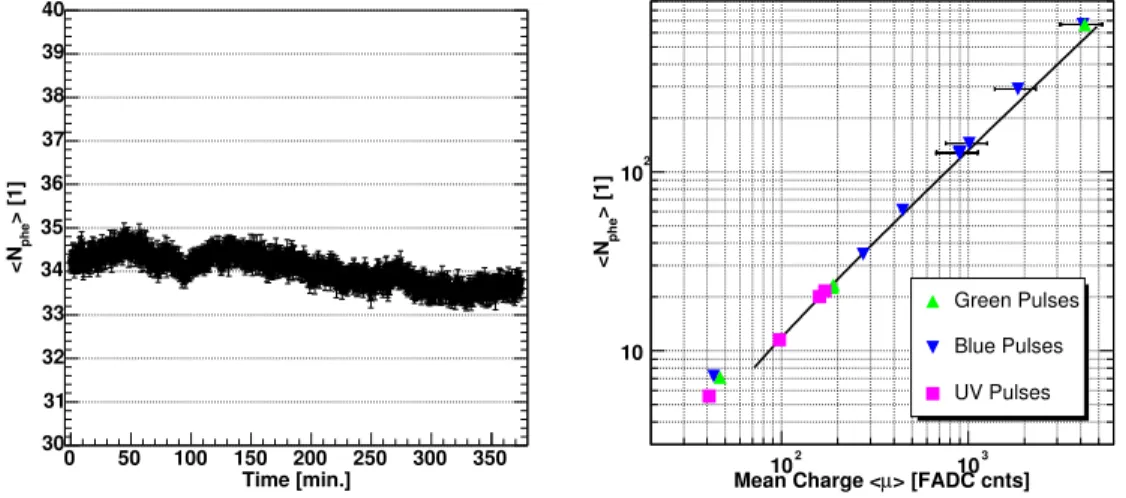
Figure 1 left shows the evolution of the mean number of photo-electrons over one night. One can see that,
102 M. Gaug et al.
despite some long-term dependency,
*: ,remains stable to about 1% on minute scales. More precise investigations revealed a dependency of the light output with ambient temperature of about 2
; 4<.
Figure 1 right shows
*=>,, calculated at different intensities and with different light colours.
Time [min.]
0 50 100 150 200 250 300 350
> [1]phe<N
30 31 32 33 34 35 36 37 38 39 40
> [FADC cnts]
µ Mean Charge <102 103
> [1]phe<N
10 102
Green Pulses Blue Pulses UV Pulses
Figure 1. Left: Evolution of the mean number of photo-electrons over one night. Right: Mean reconstructed number of photo-electrons vs. mean reconstructed charge at various intensities.
3. PIN-Diode method
We measured the absolute light flux with a PIN diode, situated at 105 cm distance from the calibration light pulser and read out with a charge sensitive pre-amplifier (shaping time 1
s) [3]. The PIN diode was calibrated with an
?Am source emitting 59.95 keV photons and a
Ba source having an emission line at 81.0 keV [5].
The assumed average energy to create an electron-hole pair by ionization is 3.62 eV at 20 C producing a peak in the recorded PIN Diode spectrum due to photo-absorption. Figure 2 shows the obtained spectra and the signals from two typical calibration light pulses. The quantum efficiency of the diode was obtained by comparison with a calibrated PIN diode. An average QE is obtained by folding the LED spectrum with the QE for each wavelength.
Table 1 shows the result of two dedicated calibration runs where both calibration methods (F-Factor and PIN Diode) have been applied to the same data. One can see a good agreement between the two results, although there is still need to reduce the systematic uncertainties (see caption).
4. Time Calibration
The photo-multipliers introduce a time delay, the “transit time (TT)”, in the amplified photo-electrons signal,
depending on the applied high-voltage (HV). Together with smaller relative delays due to different lengths of
the optical fibers, these delays have to be calibrated relatively to each other in order to obtain a correct timing
information for the analysis.
Calibration of the MAGIC Telescope 103
Table 1. Average number of photo-electrons for one pixel,calculated with both calibration methods for two different light intensities. For the PIN Diode Method, an additional systematic error of
@BADCFEHGand for the F-Factor Method,
I5% plus possible degradations of the overall PMT quantum efficiency and transmission coefficients have to be added.
Number of LEDs fired
*J>K, *=0K,F-Factor Method PIN Diode Methode
10 Leds Blue 291
L3 294
L3
20 Leds Blue 605
L6 613
L6
channel
0 50 100 150 200 250
counts
10 102 103
104 20 Leds Blue
10 Leds Blue
Am (60 keV)
241
Ba (81 keV)
133
Ba (Comp. edge 207 keV) 133
Figure 2. Spectra taken with the PIN Diode and various sources: bottom:
MONPAm with a 60 keV photon emission line, center:
P#QRQBa with a photon emission line at 81 keV and a Compton egde at 207 keV, top: the spectrum obtained from light pulses with two combinations of LEDs.
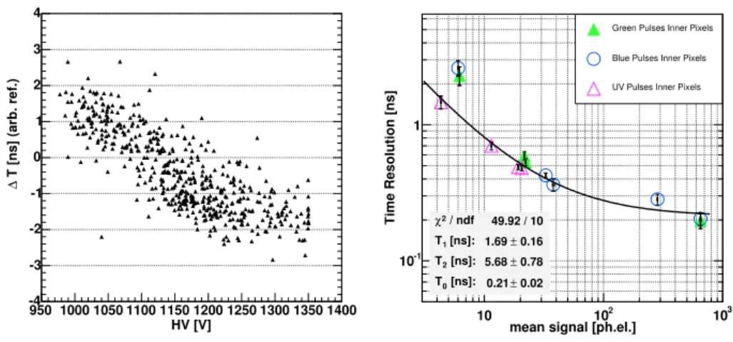
Using the light pulser at different intensities, we measured the time offsets and time spreads of the readout and detection chain. Event by event, the reconstructed arrival time difference of every channel with respect to a reference channel was measured and its mean and RMS calculated. The former yields the measured relative time offset while the latter is the convolution of the arrival time resolution of the measured and the reference channel.
Figure 3 (left) shows the time offset versus the applied HV for each PMT. Like expected, one can see a clear anti-correlation. The smaller the applied HV, the longer the signal takes to travel from the first dynode to the anode.
Figure 3 (right) shows the time resolution (RMS of the arrival time differences histogram, divided by the square root of 2), measured at different intensities. The measurements have been fitted by the following function:
S)T
U T
*=V:,
4WYXYZ)[
T
*JV:,
WYX1Z
[ T
]\
(1)
where
Tparameterizes the combination of intrinsic arrival time spread of the photons from the light pulser
and the transit time spread of the PMT,
Tparameterizes the reconstruction error due to background noise and
limited extractor resolution and
Tis a constant offset which might be due to the residual FADC clock jitter.
104 M. Gaug et al.
HV [V]
950 1000 1050 1100 1150 1200 1250 1300 1350 1400
T [ns] (arb. ref.)∆
-4 -3 -2 -1 0 1 2 3 4
mean signal [ph.el.]
10 102 103
Time Resolution [ns]
10-1
1
/ ndf χ2 49.92 / 10
[ns]:
T1 1.69 ± 0.16 [ns]:
T2 5.68 ± 0.78 [ns]:
T0 0.21 ± 0.02 / ndf χ2 49.92 / 10
[ns]:
T1 1.69 ± 0.16 [ns]:
T2 5.68 ± 0.78 [ns]:
T0 0.21 ± 0.02
Green Pulses Inner Pixels Blue Pulses Inner Pixels UV Pulses Inner Pixels
Figure 3. Left: Calibrated arrival time offsets
^&_vs. applied HV. Right: Calibrated time resolution for various intensities.
5. Conclusions
The LEDs pulser calibration system has been used to calibrate the MAGIC camera for about one year. If run in standard mode, it fires UV-pulses of 370 nm in dedicated calibration runs and additionally as interlaced calibration events with a frequency of 50 Hz. This frequency allows to accumulate enough statistics before reaching the typical time scales of residual short-term fluctuations of the optical transmission gains. The camera is such continuously monitored and re-calibrated [6] using the F-Factor method.
In dedicated calibration runs with different colours and intensities, the response of the system and signal ex- traction methods [7] have been tested.
Using a calibrated PIN Diode, the light flux of the pulser has been measured with an independent method yielding consistent results with the F-Factor method. The systematic error of both methods is still above 5%
(8% for the PIN Diode method) and will be reduced in the future.
Using the light pulses to calibrate the arrival times extracted from each channel, we find an upper limit to the time resolution of the MAGIC telescope for cosmics pulses of:
S>Ta`Rbcedgf`Rc]h
U ikj1l
*mVn,
4WYXYZ [ o(p j1l
*=Vn,
WYX1Z
[ p \p ikjql
\