Analysis of the Hadronic Calibration of the ATLAS End-Cap Calorimeters using Test Beam Data
125
0
0
Volltext
(2)
(3)
(4)
(5)
(6)
(7)
(8)
(9)
(10)
(11)
(12)
(13)
(14)
(15)
(16)
(17)
(18)
(19)
(20)
(21)
(22)
(23)
(24)
(26)
(27)
(28)
(29)
Abbildung
![Figure 1.1: The LHC accelerator chain with the location of the experiments (not to scale!) [13].](https://thumb-eu.123doks.com/thumbv2/1library_info/4011059.1541137/11.892.253.693.511.924/figure-lhc-accelerator-chain-location-experiments-scale.webp)
![Figure 1.3: Cut-away view of the ATLAS detector [14].](https://thumb-eu.123doks.com/thumbv2/1library_info/4011059.1541137/14.892.124.755.161.535/figure-cut-away-view-atlas-detector.webp)
![Figure 1.5: Sketch of a module of the EMB [30]. The dierent layers as well as the granularity in η and φ are shown.](https://thumb-eu.123doks.com/thumbv2/1library_info/4011059.1541137/18.892.229.645.200.598/figure-sketch-module-emb-dierent-layers-granularity-shown.webp)
+7
![Figure 1.8: View of an EMEC wheel [30]. Only a few example absorbers are shown.](https://thumb-eu.123doks.com/thumbv2/1library_info/4011059.1541137/19.892.281.635.187.616/figure-view-emec-wheel-example-absorbers-shown.webp)
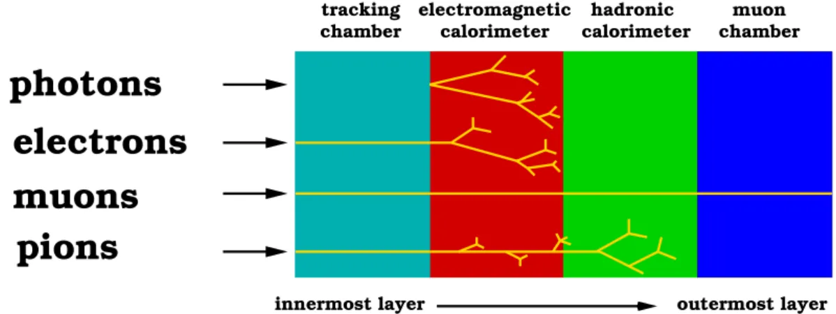
![Figure 2.3: Sketch of a hadronic shower [38]. Examples of the dierent categories of energy deposits as discussed in Section 2.4.3 are also shown.](https://thumb-eu.123doks.com/thumbv2/1library_info/4011059.1541137/26.892.181.692.709.1035/figure-sketch-hadronic-examples-categories-deposits-discussed-section.webp)
![Figure 3.1: Side view of the TB calorimeter setup in the cryostat (run 2 period) [57]](https://thumb-eu.123doks.com/thumbv2/1library_info/4011059.1541137/31.892.158.759.268.531/figure-view-tb-calorimeter-setup-cryostat-run-period.webp)
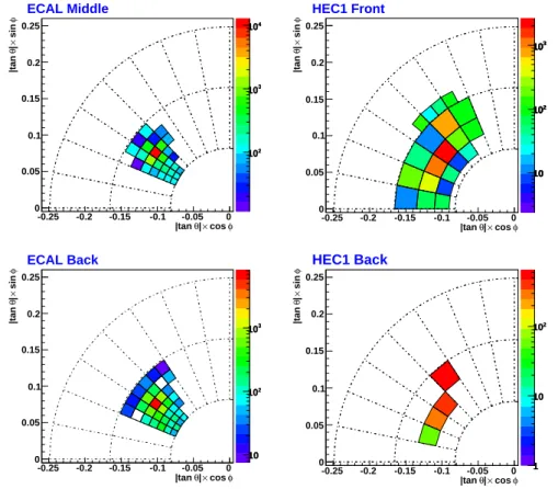
![Figure 4.3: Classication table for 2.0 < |η| < 2.2 and 8 GeV < E cluster < 16 GeV [46]](https://thumb-eu.123doks.com/thumbv2/1library_info/4011059.1541137/42.892.279.586.498.738/figure-classication-table-lt-η-gev-cluster-gev.webp)
![Figure 4.4: Average energy in DM for 500 GeV charged pions [46]. The gure represents a quarter of the ATLAS detector in a side view](https://thumb-eu.123doks.com/thumbv2/1library_info/4011059.1541137/43.892.142.764.609.1025/figure-average-energy-charged-represents-quarter-atlas-detector.webp)
ÄHNLICHE DOKUMENTE
The group of the ATLAS hadronic end-cap calorimeter (HEC) is actively involved in tests and validations of GEANT4 [3, 4]. In this talk the latest results of physics evaluation with
The size and number of the calibration regions is a trade-off between conflicting require- ments, such as the statistical and systematic errors, the time spent to collect the data,
Comparison of shower depth (left) and average cluster energy density (right) in data and MC for 200 GeV charged pions in the endcap region.. Linearity and energy resolution
Mean of the ratio of the cluster energy calibrated with hadronic weights (W), out of cluster corrections (OOC) and dead material corrections (DM) over the energy before calibration
(IEP Koˇ sice, Univ. of Montr´ eal, MPI Munich, IEAP Prague, NPI ˇ Reˇ z) The expected increase of total integrated luminosity by a factor of ten at the HL-LHC compared to the
on behalf of the ATLAS Liquid Argon Endcap Collaboration The local hadronic calibration developed for the energy reconstruction and the calibration of jets and missing transverse
Figure 14 shows the τ had-vis identification efficiencies measured in data and estimated in Monte Carlo simulation for 1-prong and 3-prong candidates for the BDT medium
New more radiation hard technologies have been studied: SiGe bipolar, Si CMOS FET and GaAs FET transistors have been irradiated with neutrons up to an integrated fluence of 2.2 · 10
