The subject of this lecture is to focus on details of the hadronic final states at low Bjorken

(1)

Christian Kiesling

Max-Planck-Institute for Physics, Munich, Germany

In this lecture we present data on hadronic final states from electron- proton reactions at low Bjorkenx, taken by the two colliding beam experiments H1 and ZEUS at HERA. The data are discussed in the context of a variety of QCD-based models, which allow for a detailed study of the QCD dynamics in the production of partons and their fragmentation into hadrons. The HERA data fully support the perturbative approach of the DGLAP evolution scheme, although some hints may be visible in certain kinematic regions for the need of alternative formulations, such as BFKL dynamics.

PACS numbers: 13.60.Hb, 13.87.Ce, 13.87.Fh, 12.38.Qk 1. Introduction

Deep inelastic scattering (DIS) of charged leptons on protons and nuclei has been an essential tool to uncover the inner structure of hadrons. The electron-proton collider HERA, unique in the world, has been the ideal place for more than 15 years to study DIS with electron and positron beams, colliding head-on with protons. On June 30, 2007, at 23:00, the HERA collider was shut down for good, ending an extremely successful period of data taking with the two colliding beam experiments H1[1] and ZEUS[2].

The subject of this lecture is to focus on details of the hadronic final states at low Bjorken

x

from electron (positron)-proton reactions at HERA.

DIS reactions sensitively probe the strong interactions of quarks and gluons (“partons”) in the kinematic regime of large momentum transfer

Q²

, e.g.

by measuring the dependence of the structure function

F₂

(x, Q

²

) on

Q²

at fixed Bjorken

x

(“scaling violations”). Such measurements can be done by observing just the scattered electron

¹

. By studying in addition the hadronic

∗lecture presented at the International School on QCD, Copanello, Calabria, Italy, July 2007.

1 here and in he following the term “electron” is used for both lepton polarities

(1)

(2)

final state, on the other hand, details of the parton dynamics, both in the perturbative and non-perturbative regime can be unraveled, as will become clear in the coarse of this lecture.

The lecture is structured as follows: First, the single particle spectra of the hadronic final state from

ep

reactions will be discussed. Then we focus on jets (collimated bundles of hadrons), which trace the original partons participating in the DIS scattering process. We will show that the measured cross sections are generally well described by the evolution of the (non- perturbative) parton distributions with

Q²

, as formulated by Altarelli and Parisi (“DGLAP” evolution). However, certain kinematic regions for jet production will be identified, where an alternative dynamics (“BFKL”) may be at work. Flavor tagging of the jets (charm and beauty) will then be discussed as well as data on prompt photons (together with jets). All these hadronic final states, with some kind of “parton identification” are called semi-inclusive. Finally we discuss some exclusive final states and present, as a warning, the story of the rise and fall of some exotic baryon resonances which, if they exist, are made out of five quarks (“pentaquarks”).

1.1. Deep Inelastic Scattering

Quantum Chromodynamics (QCD) is expected to describe the strong interactions between quarks and gluons. At distances small compared to the nucleon radius, or equivalently large momentum transfer

Q²

where the strong coupling

α

s is small, perturbative QCD (pQCD) gives an adequate quantitative account of hadronic processes. The total cross sections, how- ever, are dominated by long range forces (“soft interactions”), where a sat- isfactory understanding of QCD still remains a challenge. This is most im- portantly so also for all transitions of partons to hadrons in the final state (“fragmentation process”). In addition, non-perturbative effects govern the DIS kinematics through the momentum distribution (“parton distribution functions”, or “pdfs”) of the initial partons, interacting with the electrons via photon or

Z⁰

exchange (see fig.1). The latter is important only at very large

Q²

, i.e. around or beyond the mass of the

Z⁰

. The division between the non-perturbative and the perturbative regimes is defined by the factor- ization scale, which should be sufficiently large (

O

(few GeV

²

)to hope for a convergent perturbative expansion in the strong coupling constant

α

s.

1.2. Quantum Chromodynamics in the HERA regime

Within the framework of perturbative QCD, the DIS cross section at the parton level is generically given by

σ

=

^X

i

σ_γ^∗_i

(Q

²

)

⊗xf_i

(x), (1)

(3)

Fig. 1. Lowest order Feynman diagram for deep-inelastic electron-proton scattering in the parton picture, showing the relevant kinematical quantities char- acterizing inclusive DIS reactions (see text). The hadronic final state “frag- mented” from the scattered and spectator partons is indicated by X.

where

Q²

is the virtuality of the exchanged boson (here: the virtual photon

γ^∗

),

x

is the momentum fraction (Bjorken

x) of the incoming parton, and σγ^∗i

is the total virtual photon-parton cross section. In this expression the factorization theorem of QCD[3] has been used, separating the cross section into a hard scattering part between the exchanged virtual photon and the incoming parton

i, convoluted with a non-perturbative part describing the

momentum distribution

xfi

(x) of parton

i

within the proton. In eq.(1) one recognizes the incoherent summing of quark contributions, which is justified by the property of asymptotic freedom. Asymptotic freedom states that the interaction between the partons within the proton, characterized by the strong coupling constant

α

s become weak at large

Q²

(α s

→

0 as

Q² → ∞

).

In this way the scattering process of the electron with the partons of the proton can be treated incoherently.

Figure 1 also indicates the kinematics in the HERA regime. Here,

s

is the square of the total

ep

center of mass energy. The four-momentum transfer squared

Q²

is given by the scattered electron alone, the Bjorken variable

x

and the inelasticity

y

(equal to the energy fraction transferred from the electron to the virtual photon in the proton rest frame) are given by

Q²

=

−

(k

−k⁰

)

²

=

−q²

;

x

=

Q²

2

P ·q

;

y

=

P ·q

P ·k.

(2) Only two of the three quantities in eq.(2) are independent, they are related via

Q²

=

sxy. Another interesting quantity is the total mass MX

of the hadronic final state, given by

M_X² ≡W²

= (q +

P

)

²

=

Q²

(1

−x)

x

(3)

This relation shows that low

x

reactions correspond, at fixed

Q²

, to large

values of

W²

, i.e. large invariant masses of the hadronic final state. Due

to the high colliding beam energies (protons at 920 GeV, electrons at 27.6

GeV), HERA provided a large range of exploration for

x

and

Q²

, extending

(4)

the reach of previous fixed target experiments by more than 2 orders of magnitude in

x

and

Q²

.

The double differential cross section for

ep

scattering is written as (see, e.g. [4] )

d²σ

(e

^±p)

dx dQ²

= 2πα

² xQ⁴Y+

"

F2− y² Y+

FL∓Y⁻ Y+

xF3

#

,

(4)

where the functions

Y^±

are given by

Y^±

= 1

±

(1

−y)²

, and the structure functions, apart from coupling constants, are combinations of the parton distribution functions. For the case of pure photon exchange, valid at low

Q²

, one obtains

F₂

(x) =

^X

i=u,d,...

e²_ixf_i

(x). (5) where the sum extends over all partons within the proton of charge

ei

. As indicated in fig. 1, all reactions with neutral boson exchange are called

“neutral current (NC)” reactions, those with

W^±

exchange (here the final state lepton is a neutrino) are called “charged current (CC)” reactions.

The non-perturbative parton distribution functions

fi

(x) cannot be cal- culated from first principles and have therefore to be parameterized at some starting scale

Q²₀

. Perturbative QCD predicts the variation of

fi

with

Q²

, i.e.

fi

=

fi

(x, Q

²

) via a set of integro-differential evolution equations, as formulated by Altarelli and Parisi (“DGLAP” equations, see [5]). The pre- dicted

Q²

dependence (“scaling violations”) of the structure function

F₂

, see eq.(5), are nicely supported by the data from HERA[6].

2. General Properties of the Hadronic Final State in ep Collisions

If the hadronic final state is to be considered, one needs an additional step from the parton level discussed so far to the hadron level (“hadroniza- tion process”). This process is non-perturbative and one has to resort again to models describing this step. Similar to the parton distribution functions

fi

(x) one defines “fragmentation functions”

Di

(x

P

), giving the probability that a final state hadron carries a certain momentum fraction

xP

of the original parton

i. Such functions can be experimentally determined from

studies of single particle spectra. Also here a scale is necessary to separate, similar to the cross sections formula in eq.(1), the fragmentation from the perturbative hard collision. Also this scale is naturally called “fragmenta- tion scale” and can be chosen in the same way as the former.

The experimental investigations on the hadronic final state are preferen-

tially carried out in the so-called Breit frame, which is defined as the frame

where the virtual photon direction is collinear with the incoming charged

(5)

parton, and where the parton momentum

p^Breit

is related to the photon momentum

Q

by

p^Breit

=

Q/2. In this frame the incoming parton absorbs

the photon of momentum

−Q

and is emitted into the reverse direction with momentum

−Q/2. For this reason the Breit frame is sometimes also called

the “brick wall frame”.

Q,E* (GeV)

10 10²

p/dx± 1/N dn

0 50 100 150 200

< 0.02 0 < xp

H1 Preliminary DELPHI TASSO MARKII AMY

Q,E* (GeV)

10 10²

p/dx1/N dn

0 20 40 60 80 100

< 0.05 0.02 < xp

Q,E* (GeV)

10 10²

p/dx1/N dn

10 15 20 25 30 35

< 0.1 0.05 < xp

Q,E* (GeV)

10 10²

p/dx± 1/N dn

6 8 10 12

< 0.2 0.1 < xp

Q,E* (GeV)

10 10²

p/dx1/N dn

1 2 3 4 5

< 0.3 0.2 < xp

Q,E* (GeV)

10 10²

p/dx± 1/N dn

1 1.5 2

< 0.4 0.3 < xp

Q,E* (GeV)

10 10²

p/dx± 1/N dn

0.4 0.6 0.8 1

< 0.5 0.4 < xp

Q,E* (GeV)

10 10²

p/dx± 1/N dn

0.2 0.3 0.4

< 0.7 0.5 < xp

Q,E* (GeV)

10 10²

p/dx± 1/N dn

0.02 0.04 0.06

< 1.0 0.7 < xp

Fig. 2. Event-normalized scaled momentum distributions as functions ofQ for different x regions from H1 [7]. Also shown are data from e⁺e⁻ experiments, taking Q=E^∗ (see text).

2.1. Charged Particle Spectra

In the Breit frame two hemispheres can be defined: one in direction of the

recoiling parton, which called the “current region”, and the one into which

(6)

the “proton remainder”, i.e. the spectator di-quark system, is emitted. In the current region a single parton fragments into observable hadrons. If this fragmentation process is universal, i.e. does not depend on the way the initial partons are generated, the data from

e⁺e⁻

reactions should look very similar. In the latter case the hemispheres are divided by a plane spanned by the momentum vector of one of the final state quarks (event thrust axis).

For comparison of the results from

ep

scattering and

e⁺e⁻

it is useful to consider the scaled momentum distribution of particles, where the scaled momentum

xp

is given by

xp

= 2p

^Breit/Q. Figure 2 shows measurements [7]

of

xp

for charged particles from the H1 experiment for various values of Bjorken

x

as functions of

Q. Similar measurements also exist from the ZEUS

Collaboration [8]. The

e⁺e⁻

data are shown as well. Here, the particle momenta are rescaled to

x_p

=

p/E^∗

, where 2E

^∗

=

√

s

is the

e⁺e⁻

center of mass energy. The HERA data in the current hemisphere generally agree with the

e⁺e⁻

data, supporting quark fragmentation universality. There are, however, some kinematic regions at lower vales of

Q, where differences

are indeed expected due to higher order QCD processes, such as boson-gluon fusion or QCD Compton scattering which cannot occur in

e⁺e⁻

reactions.

Also, in the highest

Q

bin, but at low

x, there is an excess in thee⁺e⁻

data for which no evident reason exists.

In the representation of the data in fig. 2 clear scaling violations (Q

²

- dependences) are visible. Such effects can in principle be accommodated by higher order QCD calculations plus fragmentation of partons to hadrons according to some model. Various models have been tried by H1 and ZEUS (neither of them shown in the figure) and, generally, the string model of hadronization [9] gives better agreement than cluster models [10].

2.2. Strange Particle Production

An important test for the fragmentation models is the yield of strange particles, such as

K_S⁰,

Λ and ¯ Λ. Figure 3 shows the data for

K_S⁰

and Λ, Λ ¯ production from the ZEUS Collaboration [11] as functions of the transverse momentum and rapidity (similar data have been presented by the H1 Col- laboration [12] recently. Neutral strange hadrons can be identified through their displaced decay vertex and a mass fit to the observed secondaries.

The charged strange particles, such as

K^±

, are very difficult to separate

from the other charged hadrons. A significant parameter which is govern-

ing the production of strange hadrons is the strangeness suppression factor

λ_s

. It describes the probability to produce

s-quark pairs relative tou- and d-quark pairs in the string fragmentation. This parameter was determined

from

e⁺e⁻

data to be

λs

= 0.3. As can be seen from fig. 3, the ARIADNE

color dipole model (CDM) [13], implementing the Lund string fragmenta-

(7)

ZEUS

10³ 10⁴

1 1.5 2 2.5

P^LAB_T (GeV) dσ/dPLAB T (pb/GeV)

ZEUS 121 pb^-1 ARIADNE (0.3) ARIADNE (0.22) LEPTO (0.3)

5 < Q² < 25 GeV²

10³

1 1.5 2 2.5

K_S⁰

Q² > 25 GeV²

0 1000 2000 3000 4000 5000 6000 7000 8000

-1 -0.5 0 0.5 1

η^LAB dσ/dηLAB (pb)

5 < Q² < 25 GeV²

0 500 1000 1500 2000 2500 3000

-1 -0.5 0 0.5 1

Q² > 25 GeV²

ZEUS

10³ 10⁴

1 1.5 2 2.5

ZEUS 121 pb^-1 ARIADNE (0.3) ARIADNE (0.22) LEPTO (0.3)

5 < Q² < 25 GeV²

10³

1 1.5 2 2.5

Λ+Λ^–

Q² > 25 GeV²

0 500 1000 1500 2000 2500 3000 3500 4000

-1 -0.5 0 0.5 1

5 < Q² < 25 GeV²

0 200 400 600 800 1000

-1 -0.5 0 0.5 1

Q² > 25 GeV²

Fig. 3. Differential cross sections for strange hadron production from the ZEUS experiment [11] as functions of p^lab_T and η^lab. The variable η^lab is the rapidity in the lab system, defined by η=−ln tan(θ/2), whereθ is the particle’s polar angle.

The histograms show predictions from ARIADNE and LEPTO using the stated strangeness suppression factors (see text).

tion for the transition to the hadron level with the standard value for

λs

gives the best description of the data. There is no indication for any unusual yield of strange hadrons, as would be expected if QCD instanton effects [14]

were making a significant contribution.

3. Jets at HERA

Collimated bundles of particles (“jets”) are believed to carry the kine- matic information of the partons emerging from DIS reactions at HERA and other colliding beam experiments. The study of jet production is therefore a sensitive tool to test the predictions of perturbative QCD and to determine the strong coupling constant

α

s over a wide range of

Q²

.

Several algorithms exist to cluster individual final state hadrons into jets, but most commonly used at HERA is the so-called

k_T

clustering al- gorithm [15]. The jet finding is usually executed in the hadronic center of mass system. which is, up to a Lorentz boost, equivalent to the Breit frame.

At the end of the algorithm, the hadrons are collected into a number of jets.

At leading order (LO) in

α

s, di-jet production (see fig. 4) proceeds via

the QCD Compton process (γ

^∗q →qg) and boson-gluon fusion (γ^∗g→qq).

¯

The cross section for events with three jets is of

O

(α

²

s). These events can be

interpreted as coming from a di-jet process with additional gluon radiation

or gluon splitting (see caption of fig. 4), bringing the QCD calculation to

(8)

Fig. 4. Feynman diagrams for LO jet production. The upper subgraph is called “QCD Comp- ton”, the lower subgraph is called “boson-gluon fusion”. Both graphs contribute to two-jet final states. Events with three jets can be interpreted as a di-jet process with additional gluon radiation from one of the involved quark lines, or as a gluon splitting into a quark-antiquark pair.

These processes are of orderO(α²s)(NLO).

next-to-leading order (NLO).

In jet physics, two different “hard” scales can be used to enable NLO (and higher) calculations: the variable

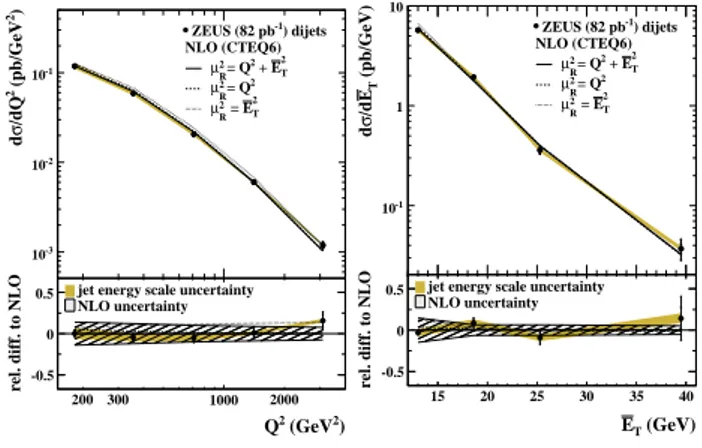
Q, and the transverse energy ET

of the jets. Figure 5 shows the differential cross sections for inclusive jet production at high

Q²

as measured by the ZEUS Collaboration [16], both with respect to

Q²

and

ET

. The data are compared to NLO calculations, using the renormalization and factorization scales as indicated in the figure.

Both schemes are able to describe the data very well, indicating the validity of the choice of any of the two hard scales. Given the experimental and theoretical uncertainties at these large scales, no higher order (beyond NLO) corrections seem necessary.

)2 (pb/GeV2/dQσd

10-3

10-2

10-1

2) (GeV Q2

200 300 1000 2000

rel. diff. to NLO^-0.5 0 0.5

) dijets ZEUS (82 pb-1 NLO (CTEQ6) 2 ET 2 +

= Q 2 µR

= Q2 2 µR

2 ET = 2 µR

jet energy scale uncertainty NLO uncertainty

(pb/GeV)TE/dσd

10-1

1 10

(GeV) ET

15 20 25 30 35 40

rel. diff. to NLO ^-0.5 0 0.5

) dijets ZEUS (82 pb-1 NLO (CTEQ6)

2 ET 2 +

= Q 2 µR

= Q2 2 µR

2 ET = 2 µR

jet energy scale uncertainty NLO uncertainty

Fig. 5. Differential cross sections for inclusive jet production from the ZEUS experiment [16]. Also shown are the predictions from next-to- leading order QCD calculations, which give a good description of the data.

3.1. The Strong Coupling Constant

One of the most important measurements using multi-jet final states

is the determination of the strong coupling constant

α

s. At HERA, this

measurement is particularly interesting, since

α

s can be determined in a

(9)

single experiment over a large range of

Q

or

E_T

. Observables which are sensitive to

α

s come from various sources, such as inclusive jets, jet ratios (number of three jets relative to the number of two jets), and event shape variables (thrust, jet masses, angles between jets etc.). A recent compilation of

α

s determinations [17] from the two HERA experiments H1 and ZEUS, using various jet observables, is shown in fig. 6. An NLO fit to these data yields a combined value of

α

s(

MZ

) = 0.1198

±

0.0019(exp.)

±

0.0026(th.).

The dominating theoretical error arises from the uncertainty due to terms beyond NLO, which is estimated by varying the renormalization scale by the “canonical” factors 0.5 and 2.

0.1 0.15 0.2

10 10²

QCD

α_s(M_Z) = 0.1189 ± 0.0010 (S Bethke, hep-ex/0606035)

(inclusive-jet NC DIS) (inclusive-jet γp) (norm. dijet NC DIS) ZEUS

ZEUS ZEUS

(norm. inclusive-jet NC DIS) (event shapes NC DIS) H1

H1

HERA αs working group

10 100

HERA

µ = Q or E

^jet_T

(GeV)

α

s

Fig. 6. Compilation of αs(µ) measurements from H1 and ZEUS [17], based on jet variables as indicated. The dashed line shows the two loop solution of the renormalization group equation, evolving the 2006 world average for αs(MZ). The band denotes the total uncertainty of the prediction.

3.2. Forward Jets

All of the analyses regarding the observables mentioned in the previous chapters rest on the DGLAP

Q²

evolution scheme for the pdfs involved.

Potential deviations observed a certain regions of phase space (low

x, low Q²

) are usually attributed to the limited order of the presently computed

QCD matrix elements (LO, NLO, sometimes NNLO). Especially for low

x

(

≈

10

⁻⁴

), but sufficiently large

Q²

(> a few GeV

²

), there has been a vivid

debate about the validity of the DGLAP approach. In this kinematic regime

the initial parton in the proton can induce a QCD cascade, consisting of

several subsequent parton emissions, before eventually an interaction with

(10)

the virtual photon takes place (see fig. 7). QCD calculations based on the

“direct” interaction between a point-like photon and a parton from the evolution chain, as given by the DGLAP approach, are very successful in describing, e.g. the unexpected rise of

F2

with decreasing

x

over a large range in

Q²

[18].

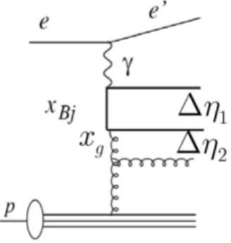
x_Bj

evolution from large

forward jet x = E

jet jet Ep Bj(small) x

to small x

(large) p

e e’

γ

Fig. 7. Schematic diagram ofepscatter- ing producing a forward jet. The evolution in the longitudinal momentum fraction x, from large xjet to small xBj, is indicated.

For low values of

x, there is, however, a technical reason to question the

validity of the DGLAP evolution approach: Since it resums only leading log(Q

²

) terms, the approximation may become inadequate for very small

x,

where log(1/x) terms become important in the evolution equations. In this region the BFKL scheme [19] is expected to describe the data better, since in this scheme terms in log(1/x) are resummed.

The large phase space available at low

x

(see eq.(3)) makes the produc- tion of forward jets (in the angular region close to the proton direction) a particularly interesting topic for the study of parton dynamics, since jets emitted in this region lie well away in rapidity from the photon end of the evolution ladder (see fig. 7). Concerning the forward jets there is a clear dy- namic distinction between the DGLAP and BFKL schemes: In the DGLAP scheme, the parton cascade resulting from hard scattering of the virtual photon with a parton from the proton is ordered in parton virtuality. This ordering along the parton ladder implies an ordering in transverse energy

ET

of the partons, so that the parton participating in the hard scatter has the highest

ET

. In the BFKL scheme there is no strict ordering in virtuality or transverse energy. The BFKL evolution therefore predicts that a larger fraction of low

x

events will contain high-E

_T

forward jets than is predicted by the DGLAP evolution.

Both ZEUS [21] and H1 [20] have studied forward jet production, where

“forward” typically means polar emission angles less than about 20 degrees

relative to the proton direction. As a first example, the single differential

cross sections

dσ/dx

from H1 are shown in fig. 8. The data are compared

to LO and NLO QCD calculations [22] (a), and several Monte Carlo models

(11)

(b and c). The NLO calculation in (a) is significantly larger than the LO calculation. This reflects the fact that the contribution from forward jets in the LO scenario is kinematically suppressed. Although the NLO contribu- tion opens up the phase space for forward jets and considerably improves the description of the data, it still fails by a factor of 2 at low

x. In fig. 8b

the predictions from the CASCADE Monte Carlo program [23] is shown, which is based on the CCFM formalism [24]. The CCFM equations pro- vide a bridge between the DGLAP and BFKL descriptions by resumming both log(Q

²

) and log(1/x) terms, and are expected to be valid over a wider

x

range. The model predicts a somewhat harder

x

spectrum, and fails to describe the data at very low

x. In part (c) of the figure, the predictions

(“RG-DIR”) from the LO Monte Carlo program RAPGAP [25] is shown, which is supplemented with initial and final state parton showers generated according to the DGLAP evolution scheme. This model, which implements only direct photon interactions, gives results similar to the NLO calcula- tions from part (a), and falls below the data, particularly at low

x. The

description is significantly improved, if contributions from resolved virtual photon interactions are included (“RG-DIR+RES”). However, there is still a discrepancy in the lowest

x

bin, where a possible BFKL signal would be ex- pected to show up most prominently. The Color Dipole Model (CDM) [13], which allows for emissions non-ordered in transverse momentum, shows a behavior similar to RG-DIR+RES.

H1 E scale uncert NLO DISENT 1+δHAD

0.5µr,f<µr,f<2µr,f

PDF uncert.

LO DISENT 1+δHAD

H1 forward jet data

x_Bj dσ / dxBj (nb)

a)

0 500 1000

0.001 0.002 0.003 0.004

H1 H1 E. scale uncert CASCADE set-1 CASCADE set-2 H1 forward jet data

b)

0 500 1000

0.001 0.002 0.003 0.004

H1 H1 E. scale uncert.

RG-DIR CDM RG-DIR+RES H1 forward jet data

c)

0 500 1000

0.001 0.002 0.003 0.004

Fig. 8. Single differential cross sections for forward jets as functions of x from the H1 experiment [20], compared to NLO predictions [22] in (a), and QCD Monte Carlo models [13, 25] in (b) and (c). The dashed line in (a) shows the LO contribution.

For a more detailed study the forward jet sample was divided into bins

of

p²_t,jet

and

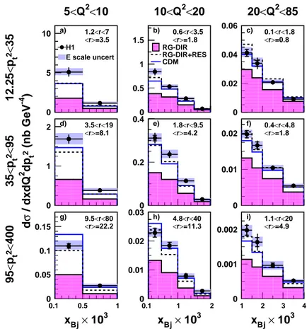
Q²

. The triple differential cross section

d³σ/dxdQ²dp²_t,jet

versus

x

is shown in fig. 9 for several regions in

Q²

and

p²_t,jet

. In addition, the

expectations from the above mentioned QCD models are presented. Using

(12)

the ratio

r

=

p²_t,jet/Q²

, various regimes can be distinguished: For

p²_t,jet <

Q²

(r < 1) one expects a DGLAP-like behavior, dominated by direct photon interactions (see fig. 9 c). Due to the large bin sizes, however, the ranges of

r

can be quite large, so that

r

in this bin can assume values up to 1.8 due to admixtures from events with

ptj² > Q²

. This may explain why the DGLAP direct model (RG-DIR), although closer to the data in this bin than in any other, does not quite give agreement with the data except at the highest

x-bin. In the region p²_t,jet ≈ Q²

(r

≈

1, see fig. 9 b and f), DGLAP suppresses parton emission, so that BFKL dynamics may show up.

However, the DGLAP resolved model (RG-DIR+RES) describes the data reasonably well.

0 5 10

0.05 0.1

x 10 ^-2 0 0.5 1 1.5

0.001 0.002 0 0.02 0.04 0.06

0.0010.0020.0030.004 0

1 2

0.05 0.1

x 10 ^-2 0 0.2 0.4

0.001 0.002 0 0.01 0.02

0.0010.0020.0030.004 0

0.05 0.1 0.15

0.05 0.1

x 10 ^-2 0 0.01 0.02 0.03

0.001 0.002

5<Q²<10

12.25<p t2<35 _H1

E scale uncert 1.2<r<7

<r>=3.5 a)

RG-DIR RG-DIR+RES CDM

10<Q²<20

0.6<r<3.5

<r>=1.8 b)

20<Q²<85

0.1<r<1.8

<r>=0.8 c)

35<p t2<95

3.5<r<19

<r>=8.1 d)

dσ / dxdQ2 dpt2 (nb GeV-4 )

1.8<r<9.5

<r>=4.2

e) 0.4<r<4.8

<r>=1.8 f)

0.1 0.5 1

95<p t2<400

9.5<r<80

<r>=22.2 g)

x_Bj× 10³

0.1 1 2

4.8<r<40

<r>=11.3 h)

x_Bj× 10³

1 2 3 4

1.1<r<20

<r>=4.9 i)

x_Bj× 10³

0 0.001 0.002

0.0010.0020.0030.004

Fig. 9. Triple differential cross sections for forward jet production as function of x in bins ofQ² andp²_t,jet, compared to various Monte Carlo calculations (see text).

The regime of

p²_t,jet> Q²

(r > 1, see fig. 9 d, g and h), is typical for pro-

cesses where the virtual photon is resolved, i.e. the incoming parton from

(13)

the proton vertex interacts with a parton from the photon. As expected, the DGLAP resolved model (RG-DIR+RES) provides a good overall de- scription of the data, again similar to the CDM model. However, it can be noted that in regions where

r

is largest and

x

is small, CDM shows a tendency to overshoot the data. DGLAP direct (RG-DIR), on the other hand, gives cross sections which are too low. Although the above anal- ysis tries to isolate “BFKL regions” from “DGLAP regions”, the conclu- sion on underlying dynamics cannot be reached, most importantly since the

“BFKL region” (r

≈

1) is apparently heavily contaminated by “DGLAP- type” events. In addition, the two “different” evolution approaches, RG- DIR+RES (“DGLAP”) and CDM (“BFKL”), give similar predictions.

Fig. 10. Kinematic regions for the event sample

“2jets + forward” (see text). The quarks in the photon-gluon fusion process are q1 (upper solid line) and q2 (lower solid line). The rapidity gap betweenq1andq2is denoted by∆η1, the gap between q2 and the forward jet is denoted by ∆η2.

In a further step, the parton radiation ladder (see fig. 7) is exam- ined in more detail by looking also at jets in the region of pseudorapid- ity,

η

=

−

ln tan(θ/2), between the scattered electron (η

e

) and the forward jet (η

_forw

). In this region a “2-jet + forward” sample was selected, re- quiring at least 2 additional jets, with

p_t,jet >

6 GeV for all three jets, including the forward jet. In this scenario, evolution with strong

k_t

order- ing is obviously disfavored. The jets are ordered in rapidity according to

ηforw > ηjet2 > ηjet1 > ηe

. Two rapidity intervals are defined between the two additional jets and the forward jet (see fig. 11): ∆η

1

=

ηjet2−ηjet1

is the rapidity interval between the two additional jets, and ∆η

2

=

ηforw−ηjet2

is the interval between jet 2 and the forward jet. If the di-jet system originates from the quark line coupling to the photon (see fig. 11), the phase space for evolution in

x

between the di-jet system and the forward jet is increased by requiring that ∆η

1

is small and that ∆η

2

is large: Requiring ∆η

1 <

1 will favor small invariant masses of the di-jet system. As a consequence,

x_g

will be small, leaving the rest for additional radiation. When, on the other hand, ∆η

₁

is required to be large (∆η

₁ >

1) BFKL-like evolution may then occur between the two jets from the di-jet system or, when both ∆η

1

and

∆η

2

are small, between the di-jet system and the hard scattering vertex.

Note that the rapidity phase space is restricted only for the forward jet.

(14)

∆η₂ dσ/d∆η2 (nb)

All ∆η₁

H1

E scale uncert.

RG-DIR CDM RG-DIR+RES

a)

0 0.02 0.04 0.06

0 2

∆η₁<1

∆η₂ dσ / d∆η2 (nb)

b)

0 0.01 0.02

0 2

∆η₁>1

∆η₂ dσ / d∆η2 (nb)

c)

0 0.01 0.02 0.03

0 2

Fig. 11. Cross section for events with a reconstructed high transverse momentum di-jet system and a forward jet from the H1 experiment [20], as function of ∆η2

for two regions of ∆η1. The data are compared to predictions of “DGLAP-like (RG-DIR+RES) and “BFKL-like” (CDM) Monte Carlo models (see text).

As argued above, this study disfavors evolution with strong ordering in

kt

due to the common requirement of large

pt,jet

for the three jets. Radiation which is not ordered in

kt

may occur at any location along the evolution chain, depending on the values of ∆η

1

and ∆η

2

. Figure 11 show the mea- sured cross sections as function of ∆η

2

for all data, and separated into the two regions of ∆η

1

discussed above. One can see that here the CDM model is in good agreement with the data in all cases, while the DGLAP models predict cross sections which are too low, except when both ∆η

₁

and ∆η

₂

are large. For this topology all models (and the NLO calculation, not shown) agree with the data, indicating that the available phase space for evolution is exhausted.

It is important to realize that the “2+forward jet” sample indeed seems to differentiate between the CDM and DGLAP resolved models, in contrast to the more inclusive samples (see fig. 9). The conclusion is that additional breaking of the

k_t

ordering, beyond what is included in the resolved photon model, is required by the data, pointing towards some evidence for BFKL dynamics. It is, however, not excluded that such effects may also be de- scribed by higher order DGLAP calculations, which may become available in the future.

4. Open Charm and Beauty Production

Low

x

physics processes at HERA are dominated by gluonic contribu-

tions and are therefore governed by the gluon distribution function within

the proton. This function can be determined indirectly from the scaling

(15)

violations of the structure function

F₂

, as measured in DIS inclusive

ep

scattering (see, e.g., [26] for recent results on pdfs from a QCD fit to the combined data of H1 and ZEUS). A more direct way to access the gluon dis- tribution is to select boson-gluon fusion processes (see fig. 4, lower graph).

In order to suppress the QCD Compton part (fig. 4, upper graph), the quark loop should contain heavy quarks not present in the proton, i.e. charm or bottom quarks. The production of

c

and

b

quarks in

ep

collisions also pro- vides stringent tests for perturbative QCD, since the heavy quark masses (m

²_c ≈

10 GeV

²

,

m²_b ≈

25 GeV

²

) can serve as hard scales to ensure reliable perturbative calculations.

Heavy quarks in the final state are identified by various methods:

c

quarks are usually identified by explicit reconstruction of a

D^∗

meson. Such methods, however, drastically reduce the statistics due to the small branch- ing ratios into particular final states. For

b

quarks, explicit reconstruction at HERA is impossible due to lack of statistics in any of the very many ex- clusive final states. Production of hadrons with

b-quarks, however, can be

enhanced by requiring the presence of one or more jets, tagged by a muon or electron from the semileptonic decay of one of the

b

quarks.

There is an alternative method to tag heavy quark production: With the help of high-precision micro-vertex detectors, mesons containing heavy quarks are distinguished from those containing only light quarks by recon- structing the displacement of the decay tracks from the primary vertex, caused by the short (but finite) lifetime of these mesons. The clear advan- tage of this method is that all decay channels of the charm/bottom hadrons can be used and the phase space for heavy quark selection need not be restricted. A problem, however, is to separate charm from bottom, in par- ticular at low

Q²

, since the

b

production at HERA is expected to be small compared to charm.

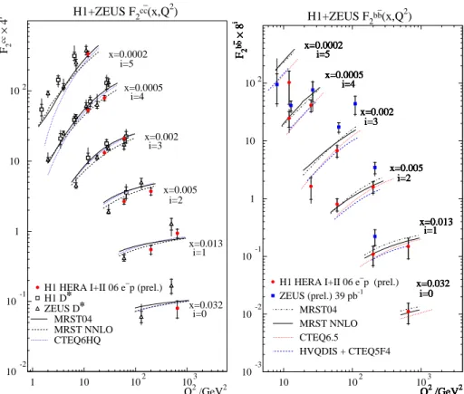
Figure 12 shows the data from H1 [27] and ZEUS[28] on the structure functions

F₂^cc

and

F₂^bb

, which are derived from the reduced cross section, dividing out the kinematic terms divided given in eq.(4), according to

˜

σ_c¯_c,b¯b ≡ d²σ^c¯^c,b^¯^b dxdQ²

xQ⁴

2πα(1 + (1

−y)²

)

!

=

F₂^c¯^c,b^¯^b− y²

1 + (1

−y)²F_L^c¯^c,b^¯^b.

(6)

Here, the small contribution from the longitudinal structure function

F_L^c¯^c,b^¯^b

is estimated from NLO QCD predictions [29, 30], based on the variable

flavor number scheme (VFNS), to be discussed subsequently. Also shown

are previous measurements for

F₂^cc

from H1 [31] and ZEUS [32] based on

D^∗

tagging. Due to the limited acceptance for clean reconstruction of

D^∗

’s

in the final state, the data need to be extrapolated to the full solid angle,

which has been done by using an NLO program [33] for charmed quark pair

(16)

H1+ZEUS F₂^cc^_(x,Q²)

10^-2 10^-1 1 10 10²

1 10 10² 10³

x=0.0002 i=5

x=0.0005 i=4

x=0.002 i=3

x=0.005 i=2

x=0.013 i=1

x=0.032 i=0 H1 HERA I+II 06 e⁻p (prel.) H1 D^✽

ZEUS D^✽ MRST04 MRST NNLO CTEQ6HQ

Q² /GeV²

F2cc_ × 4i H1+ZEUS F₂^bb

_

(x,Q²)

10^-3 10^-2 10^-1 1 10 10²

10 10² 10³

x=0.0002 i=5

x=0.0005 i=4

x=0.002 i=3

x=0.005 i=2

x=0.013 i=1

x=0.032 i=0

Q² /GeV² F2bb_ × 8i

x=0.0002 i=5

x=0.0005 i=4

x=0.002 i=3

x=0.005 i=2

x=0.013 i=1

x=0.032 i=0

x=0.0002 i=5

x=0.0005 i=4

x=0.002 i=3

x=0.005 i=2

x=0.013 i=1

x=0.032 i=0

x=0.0002 i=5

x=0.0005 i=4

x=0.002 i=3

x=0.005 i=2

x=0.013 i=1

x=0.032 i=0

x=0.0002 i=5

x=0.0005 i=4

x=0.002 i=3

x=0.005 i=2

x=0.013 i=1

x=0.032 i=0

x=0.0002 i=5

x=0.0005 i=4

x=0.002 i=3

x=0.005 i=2

x=0.013 i=1

x=0.032 i=0

H1 HERA I+II 06 e⁻p (prel.) ZEUS (prel.) 39 pb^-1

MRST04 MRST NNLO CTEQ6.5

HVQDIS + CTEQ5F4

Fig. 12. Structure functionsF₂^cc andF₂^bb as function ofQ² for various values ofx from HERA (see text). The QCD predictions differ mainly by their pdfs.

production, based on DGLAP evolution.

The data from the two experiments are in reasonable agreement and also agree with the previous measurements using

D^∗

tagging. There is a ten- dency, however, for the ZEUS data to lie above the H1 data, both for charm and bottom production. Comparisons are made with the above mentioned NLO QCD predictions, which are able to describe the data. The precision of the data is not yet sufficient to distinguish between the predictions, which are based on different pdfs.

For the comparison of QCD with the measurements of the structure

function

F₂^c¯^c,b^¯^b

one has to choose DIS events to have a hard scale, here

Q²

. For

b

quark production, however, DIS is plagued with very low cross

sections, so that stringent tests of QCD models is hampered by low statis-

tics. A way to substantially increase the statistics is to go down in

Q²

(photoproduction) and select a different hard scale for the comparison with

perturbative QCD calculations. Such a scale can be provided by considering

(17)

jet production with

b-quarks (hard scale is E_T

of the jet), or even forget about the jet selection to increase the statistics even more, and use the mass of the

b-quark itself as the hard scale. An interesting analysis of the latter

type has been presented by the ZEUS collaboration [34], looking into events with two muons, without any requirement on jets or

pt

of the muons.

The principle of selecting an almost background-free sample with

b-quark

production is to look for like-sign di-muon events. Like-sign di-muons can only originate from the decays of different

b-quarks, where one µ

is from a semileptonic

b-quark decay, and the otherµ

is from the semileptonic ¯

c

decay (after a hadronic decay of the ¯

B-hadron in an anti-charmed meson). Unlike-

sign muons come from the same parent

B

hadron, e.g. through the decay chain

b→ cµX →sµµX⁰

, or from the semileptonic decays of the

B

and ¯

B

hadrons. Beauty production is the only source of genuine like-sign muons, backgrounds from light flavors are well controlled, contributing equally to like-sign and unlike-sign di-muon events.

Fig. 13. Measured differential cross sections for b-quark production as function of pt of the b-quark, summarizing all photoproduction data from HERA [35]. Also shown is the corresponding NLO expectation (see text).

Figure 13 shows a recent compilation of the differential cross section for

b-quark photoproduction for all HERA data [35] together with the NLO

expectation [36]. In contrast to DIS

c-quark production, where the theory

is in agreement with the measurement (not shown here), the prediction for

b-quark photoproduction is lower by about a factor of 2 over most of thep_t

range. As can be seen, the data from H1 [37] agree with the ZEUS data. A

similar factor, in mutual agreement, has also been found in deep-inelastic

production of

b-quarks by H1 [38] and ZEUS [39].

(18)

5. Prompt Photons

Photons originating from partonic interactions provide a sensitive probe for precision tests of perturbative QCD and yield information on the struc- ture of the proton, when they are radiated from the quark lines. Such photons, coupling to the interacting partons, are often called “prompt”, as opposed to photons from hadron decays or photons radiated by leptons. In contrast to measurements using hadrons, prompt (or isolated) photons min- imize uncertainties from parton fragmentation, hadronization or jet identifi- cation. Furthermore, the experimental uncertainties of the energy measure- ment are smaller for electromagnetic showers initiated by photons than for hadronic showers initiated by jets. On the other hand, there is a substantial background coming from

π⁰

decays, which outnumber the prompt photons by a large factor.

[cm]

Transversal

Radius

2 4 6

Photon Candidates

0 500 1000 1500 2000

[cm]

Transversal

Radius

2 4 6

Photon Candidates

0 500 1000 1500 2000

H1

preliminary

Isolated Photons in DIS Fig. 14. Distribution of the transverse cluster radius for photon candidates from the H1 analysis [40].

Also shown are the contributions from π⁰ decay (shaded histogram), the photons radiated off the lepton line (thin solid histogram, and the contribution from the “prompt”

photons, radiated off the quark line (dashed histogram).

The isolated photon signal can be extracted in several ways. The one used by H1 [40] exploits the fine granularity LAr calorimeter information in order to determine a number of “shower shape variables” from the iso- lated electromagnetic clusters associated with photon candidates. ZEUS [41]

uses its presampler in front of the barrel electromagnetic calorimeter to con- vert the photons to

e⁺e⁻

pairs. For the case of H1, fig. 14 shows one of six shower shape variables, which characterizes the transverse size of the photon shower. The data are compared to the expectation from various sources, using the properly adjusted Monte Carlo simulations RAPGAP [25]

for the photons from the electron line (“LL”,thin solid histogram), and

PYTHIA [42] for the prompt photons from the quark line (“QQ”, dashed

histogram). The

π⁰

background is simulated in both LO programs at the

end of a parton shower step with subsequent Lund string fragmentation

into final state hadrons (shaded histogram). The thick solid histogram, well

describing the data, is the sum of all contributions.

(19)

Fig. 15. Differential cross section for the production of isolated photons as functions of η^γ andQ². The NLO calculations [43] are also shown (see text).

Figure 15 shows the differential cross section for isolated photon pro- duction as function of the photon rapidity

η^γ

and

Q²

at the electron vertex.

The data are compared with a LO (

O

(α

³

)) calculation [43], where the in- dividual contributions from the lepton line, the quark line and the sum, including the interference term, are shown. The prediction underestimates the data by almost a factor of 2, clearly indicating the need for higher order corrections in the pQCD calculation. The prediction comes closer to the data, when in addition to the prompt photon a jet is required.

6. Specific Final States

All the differential cross sections for inclusive or semi-inclusive hadronic final states in

ep

reactions discussed so far were characterized by a hard scattering (short distance) process at the parton level, which provided the basis for their theoretical description within the framework of perturbative QCD. The total cross section, on the other hand, is dominated by soft in- teractions, characterized by an almost energy-independent cross section. A large fraction of these soft interactions is mediated by color-singlet (vacuum quantum number) exchange, and is termed “diffractive”. In hadronic in- teractions, diffraction is well described by Regge theory (see, e.g. [44] for a review). In Regge theory, diffractive processes are formulated as a

t-channel

exchange of a leading trajectory with vacuum quantum numbers, called the

“Pomeron” trajectory. In the high energy limit, Pomeron exchange dom- inates over all other contributions to the scattering amplitude and thus represents an essential non-perturbative feature of strong interactions.