Search for diboson resonances in hadronic final states in 139 fb − 1 of p p collisions at √

A TLAS-CONF-2019-003 20/05/2019

ATLAS CONF Note

ATLAS-CONF-2019-003

20th May 2019

Search for diboson resonances in hadronic final states in 139 fb ^{− 1} of p p collisions at √

s = 13 TeV with the ATLAS detector

The ATLAS Collaboration

Narrow resonances decaying into WW , W Z or Z Z boson pairs are searched for in 139 fb

of proton–proton collision data at a centre-of-mass energy of

√ s = 13 TeV recorded with the ATLAS detector at the Large Hadron Collider from 2015 to 2018. The diboson system is reconstructed using pairs of high transverse momentum, large-radius jets. These jets are built from a combination of calorimeter- and tracker-inputs compatible with the hadronic decay of a boosted W or Z boson, using jet mass and substructure properties. The search is performed for diboson resonances with masses greater than 1.3 TeV. No significant deviations from the background expectations are observed. Exclusion limits at the 95% confidence level are set on the production cross-section times branching ratio into dibosons for resonances in a range of theories beyond the Standard Model, with the highest excluded mass of a new gauge boson at 3.6 TeV in the context of mass-degenerate resonances that couple predominantly to gauge bosons.

Erratum: The limit plots in the version dated 17th March 2019 wrongly showed σ(pp → V

) × BR (V

→ VV ) × BR (V → qq) × BR (V → qq) instead of σ(pp → V

) × BR (V

→ VV) (and equivalent for bulk RS and radion models). The new results are corrected for this and are now based on pseudo experiments.

© 2019 CERN for the benefit of the ATLAS Collaboration.

Reproduction of this article or parts of it is allowed as specified in the CC-BY-4.0 license.

1 Introduction

The discovery of new phenomena in high-energy proton–proton ( pp ) collisions is one of the main goals of the Large Hadron Collider (LHC). New heavy, TeV-scale, resonances of vector bosons VV (where V represents a W or a Z boson) are a possible signature of such new physics and are predicted in several extensions to the Standard Model (SM). These include extended gauge-symmetry models [1–3], Grand Unified theories [4–7], theories with warped extra dimensions [8–12], two-Higgs-doublet models [13], little-Higgs models [14], theories with new strong dynamics [15], including technicolour [16–18], and more generic composite Higgs models [19]. The data sample of 36.7 fb

of pp collisions collected in 2015 and 2016 at the LHC at

√ s = 13 TeV offered improved sensitivity to heavy diboson resonances compared with earlier results. The ATLAS and CMS collaborations performed searches in the fully hadronic final states using this data [20, 21] but no significant deviation from a smooth background consistent with the SM expectation was observed. Searches by ATLAS [22, 23] and CMS [24, 25] for semileptonic decay modes of the boson pair, as well as statistical combinations of various decay channels [26], on the same data also did not reveal any hint of new physics.

This paper presents a search for narrow diboson resonances decaying into fully hadronic final states in 139 fb

of pp collision data collected by the ATLAS experiment between 2015 and 2018. The W and Z bosons produced in the decay of TeV-scale resonances are highly boosted, and are therefore reconstructed in ATLAS as a single large-radius-parameter jet. The signature of such heavy resonance decays is thus a resonant structure in the dijet invariant mass spectrum. Although the hadronic decays of vector bosons have the largest branching ratio (67% for W and 70% for Z bosons), they suffer from background contamination from the production of multijet events. This background is larger by several orders of magnitude, and to suppress it, the characteristic jet substructure of W/Z boson decays is used. Contributions to the background from SM processes containing bosons, V + jets, SM VV , t t ¯ and single top production, are significantly smaller.

To improve the sensitivity of this search, new techniques are used. Novel inputs are used for jet finding, which improve the jet substructure resolution of ATLAS in highly boosted topologies [27]. To further benefit from these developments, a new approach for identifying boosted boson candidates is introduced.

The identification of the boosted boson candidates is validated using the known SM V + jets production.

To avoid limitations caused by poor modelling or limited numbers of Monte Carlo (MC) generated

background events, the observed background is characterised by a parametric function fit to the smoothly

falling dijet invariant mass distribution. To assess the sensitivity of the search, to optimise the event

selection and for comparison with the observed data, three specific benchmark models are used: a spin-0

radion [28] decaying into WW or Z Z ; a spin-1 Heavy Vector Triplet (HVT) Model [29] that provides

signals such as W

→ W Z and Z

→ WW ; and a spin-2 graviton G

→ WW or Z Z , corresponding to

Kaluza–Klein (KK) modes [8, 9] of the Randall–Sundrum (RS) graviton [10–12]. These models assume

production mechanisms either via gluon–gluon fusion or quark–antiquark annihilation.

2 ATLAS detector

The ATLAS detector [30] surrounds nearly the entire solid angle around the ATLAS collision point. It has an approximately cylindrical geometry1 and consists of an inner tracking detector surrounded by electromagnetic and hadronic calorimeters and a muon spectrometer. The tracking detector is placed within a 2 T axial magnetic field provided by a superconducting solenoid and measures charged-particle trajectories with silicon pixel and silicon microstrip detectors that cover the pseudorapidity range |η| < 2 . 5, and with a straw-tube transition radiation tracker covering |η | < 2 . 0. A new innermost pixel layer [31, 32]

inserted at a radius of 3.3 cm has been used since 2015.

Electromagnetic and hadronic calorimeter systems provide energy measurements with high granularity.

The electromagnetic calorimeter is a liquid-argon (LAr) sampling calorimeter with lead absorbers, spanning

|η| < 3 . 2 with barrel and endcap sections. The three-layer central hadronic calorimeter comprises scintillator tiles with steel absorbers and extends to |η| = 1 . 7. The hadronic endcap calorimeters measure particles in the region 1 . 5 < |η| < 3 . 2 using liquid argon with copper absorbers. The forward calorimeters cover 3 . 1 < |η| < 4 . 9, using LAr/copper modules for electromagnetic energy measurements and LAr/tungsten modules to measure hadronic energy.

The muon spectrometer surrounds the calorimetry system and provides precision muon tracking and triggering. It includes three large superconducting air-core toroids providing a magnetic field for accurate momentum measurements in tracking drift chambers arranged in a barrel, covering |η | < 1 . 0, and endcaps, extending to |η| = 2 . 7.

Events are recorded in ATLAS if they satisfy a two-level trigger requirement [33]. The level-1 trigger detects jet and particle signatures in the calorimeter and muon systems with a fixed latency of 2.5 µ s, and is designed to reduce the event rate to about 100 kHz. Jets are identified at level-1 with a sliding-window algorithm, searching for local maxima in square regions with size ∆ η × ∆ φ = 0 . 8 × 0 . 8. The subsequent high-level trigger consists of software-based trigger filters that reduce the event rate to one kHz.

3 Data

The search is performed using data collected by the ATLAS experiment from 2015 to 2018 from √ s = 13 TeV LHC pp collisions. Events used in this search satisfied a single-jet trigger requiring at least one jet reconstructed at each trigger level. The final filter in the high-level trigger required a jet to satisfy a high transverse momentum ( p

) threshold, p

≥ 360 GeV (2015), p

≥ 420 GeV (2016), p

≥ 440 GeV (2017 and 2018), reconstructed with the anti- k

algorithm [34] and a large radius parameter ( R = 1 . 0).

Calorimeter-cell energy clusters calibrated to the hadronic scale utilising the local cell signal weighting method [35] were used as inputs. After requiring that the data were collected during stable beam conditions and the detector components relevant to the analysis were functional, the integrated luminosity was 3.2 fb

in 2015, 33.0 fb

in 2016, 44.3 fb

in 2017 and 58.5 fb

in 2018.

1

ATLAS uses a right-handed coordinate system with its origin at the nominal interaction point (IP) in the centre of the detector and the

-axis along the beam pipe. The

-axis points from the IP to the centre of the LHC ring, and the

-axis points upward. Cylindrical coordinates

are used in the transverse plane,

being the azimuthal angle around the beam pipe.

The pseudorapidity is defined in terms of the polar angle

as

ln tan

2

Angular distance is measured in units of

∆R=p

(∆η)2+(∆φ)2

.

4 Simulation

4.1 Signal Models

MC simulation of signal events is used to optimise the sensitivity of the search and to interpret its results.

Signals are simulated in three benchmark scenarios.

In the first scenario, the gravitational fluctuations in the extra dimension of the Randall–Sundrum framework correspond to scalar fields, known as the radion, which are massless in the simplest scenario. A fundamental problem in the original Randall–Sundrum framework is that it lacks a mechanism to stabilise the radius of the compactified extra dimension, r

. One possible mechanism to achieve this is to introduce an additional bulk scalar radion, produced via gluon–gluon fusion, which has its interactions localised on the two ends of the extra dimension [36, 37]. This causes the radion field to acquire a mass term, which is typically much smaller than the first KK excitation mass. The coupling of the radion field to SM fields scales inversely proportional to the model parameter Λ

= √

g × k × e

q

M

5

/k

where M

is the 5-dimensional Planck mass, which has been extensively studied in the literature [28, 38, 39], k the curvature factor, and g is the 5-dimensional metric. The size of the extra dimension, defined as k πr

, is another parameter of the model.

In this analysis, the curvature factor is set to kπr

= 35, and Λ

= 3 TeV is used.

The couplings of the radion to fermions are proportional to the masses of the fermions, while the couplings are proportional to the square of the masses for bosons. For radion mass above ∼ 1 TeV, the dominant decay mode is into pairs of bosons. The decay width of the radion is approximately 10% of its pole mass, resulting in observable mass peaks with a width comparable to the experimental resolution (see Section 6.3). The calculated production cross-section times branching ratio ( σ × B ) for a radion decaying into WW , with the W decaying hadronically, is 2.75 fb and 0.26 fb for radion masses of 2 TeV and 3 TeV, respectively. Corresponding values for a radion decaying into Z Z are 1.53 fb and 0.15 fb.

The second scenario is based on two benchmark models, A and B, of the HVT phenomenological Lagrangian [29]. The Lagrangian introduces a new heavy vector triplet V

, where V

refers to W

and Z

, produced via quark–antiquark annihilation, whose members are degenerate in mass, and parameterises its couplings to SM fields in a generic manner, such that a large class of extensions to the SM can be described.

Model A with the strength of the vector-boson interaction g

= 1 [29] describes scenarios where the new triplet field couples weakly to the SM fields and arises from an extension of the SM gauge group, with the heavy vector bosons having comparable branching ratios into fermions and gauge bosons. For W

and Z

masses of interest, the width of the new heavy bosons is approximately 2.5%, which results in observable mass peaks with a width dominated by the experimental resolution. The branching fraction of the new heavy boson W

( Z

) to each of the W Z and W H ( WW and Z H ) final states, where H represents the Higgs boson, is approximately 2%. The calculated σ × B values for W

→ W Z , with W and Z bosons decaying hadronically, are 8.3 fb and 0.75 fb for W

masses of 2 TeV and 3 TeV, respectively. Corresponding values for Z

→ WW are 3.8 fb and 0.34 fb.

Model B with g

= 3 is representative of composite Higgs models, where the fermionic couplings to

V

are suppressed. For the W

and Z

masses of interest, the branching fraction of the new heavy boson

W

( Z

) to each of the W Z and W H ( WW and Z H ) final states is close to 50%. Resonance widths and

experimental signatures are similar to those obtained for model A and the predicted σ × B values for

W

→ W Z , with hadronic W and Z decays, are 13 fb and 1.3 fb for W

masses of 2 TeV and 3 TeV, respectively. Corresponding values for Z

→ WW are 6.0 fb and 0.55 fb.

The third scenario considered is the bulk RS model [10] that extends the original RS model [8, 40] with a warped extra dimension, by allowing the SM fields to propagate in the bulk of the extra dimension. This model is characterised by a dimensionless coupling constant κ/M

∼ 1, where κ is the curvature of the warped extra dimension, and M

is the reduced Planck mass. In this model, a Kaluza–Klein graviton, G

, predominately produced via gluon–gluon fusion, decays into pairs of top quarks, pairs of Higgs bosons, WW and Z Z with significant branching fractions. The branching fraction of the G

to WW ( Z Z ) ranges from 24% to 20% (12% to 10%) as the mass increases. The decay width of the G

is approximately 6% of its pole mass, resulting in observable mass peaks with a width comparable to the experimental resolution, and σ × B for G

→ WW , with the W decaying hadronically, is 1.29 fb and 0.06 fb for G

masses of 2 TeV and 3 TeV, respectively. Corresponding values for G

→ Z Z are 0.65 fb and 0.03 fb.

4.2 Simulated event samples

For all MC samples, all hadronic decays were imposed at the generator level. MC samples for the radion, HVT, and RS models, were generated using MadGraph 2.2.2 [41] interfaced to Pythia 8.186 [42] for hadronisation using the leading-order (LO) NNPDF 2.3 parton distribution function (PDF) set [43] and the ATLAS A14 set of tuned parameters for the underlying event [44]. In all signal samples, the W and Z bosons are primarily longitudinally polarised. The procedure to derive the optimal boson identification criteria (Section 6.1) uses a dedicated sample of W

decaying only into W/Z bosons that in turn decay hadronically. Pythia 8.186 was used to generate this sample with the A14 set of tuned parameters for the underlying event and the NNPDF 2.3 LO PDF. The cross-section of the hard-scattering process was modified by applying an event-by-event weighting factor to broaden the width of the resonance and widen the p

distribution of the electroweak bosons produced in its hadronic decays.

Pythia 8.186 with the NNPDF 2.3 LO PDF set and the A14 set of tuned parameters was used to generate and shower multijet background events. Samples of W +jets and Z +jets events were generated with Sherpa 2.2.5 [45–48] interfaced with the NNPDF 3.0 next-to-next-to-leading-order (NNLO) PDF set [49].

A t t ¯ sample generated with Powheg-Box v2 [50–52] with the NNPDF 3.0 next-to-leading-order (NLO) PDF [53], interfaced with Pythia 8.186 with the NNPDF 2.3 LO PDF and the A14 set of tuned parameters for parton showering is used for the V +jets study. EvtGen v1.2.0 [54] was used for properties of bottom and charm hadron decays, except for samples generated by Sherpa.

For all MC samples, the final-state particles produced by the generators were propagated through a detailed detector simulation based on GEANT4 [55, 56]. The mean number of pp interactions per bunch crossing,

‘pile-up’, was approximately 33 in the collision data being used for the analysis. The expected contribution

from these minimum-bias pp interactions was accounted for by overlaying additional minimum-bias events

generated with Pythia 8.186 using the ATLAS A3 [57] set of tuned parameter. The MC simulation events

were weighted to match the distribution of the average number of interactions per bunch crossing observed

in collision data. Simulated events were then reconstructed with the same algorithms as run on the collision

data.

5 Reconstruction

The experimental signatures central to this analysis are hadronic jets. Since the decay products of TeV-scale resonances are highly boosted, their decay products become increasingly collimated and they are therefore reconstructed as a single large-radius jet. It is important that they can still be differentiated from multijet events where a jet is initiated by a single quark or gluon. This relies on both the energy and angular resolution of the detector used to reconstruct the jet. Although the analysis primarily relies on jets, reconstruction of lepton candidates is necessary to reject events that could bias the SM V +jets studies presented in Section 6.2.

5.1 Track-CaloClusters

In previous analyses, ATLAS has mainly focused on the use of calorimeter-based jet substructure, which exploits the exceptional energy resolution of the ATLAS calorimetry [35]. However, as the event becomes even more energetic, jets become so collimated that the calorimeter lacks the angular resolution to resolve the desired structure inside the jet. For boson jets with high transverse momentum, p

, only a handful of calorimeter-cell clusters are created, each with limited angular resolution, but excellent energy resolution.

On the other hand, the tracking detector has excellent angular resolution and good reconstruction efficiency at very high energy [58], while its momentum resolution deteriorates. By combining information from the ATLAS calorimeter and tracking detectors, the precision of jet substructure techniques can be improved for a wide range of energies. This analysis uses a new unified object built from both the tracking and the calorimeter information, referred to as Track-CaloClusters (TCCs) [27]. This procedure is a type of particle flow, complementary to the energy subtraction algorithm described in the ATLAS particle flow paper [59] which improves the energy resolution of low-energy jets. The two algorithms are designed to improve the jet reconstruction performance in very different energy regimes, reflected in their distinct four-momentum construction and energy sharing procedures. Energy sharing in the TCC approach is based solely on a weighting scheme where only the relative track momenta are used to spatially redistribute the energy measured in the calorimeter. In practice, this means that the TCC algorithm uses the spatial coordinates of the tracker and the energy scale of the calorimeter. A more detailed description of TCCs can be found in Ref. [27].

5.2 Jet reconstruction

This analysis uses anti- k

, R = 1 . 0 jets reconstructed from both the combined and the neutral TCCs.

Combined TCCs are four-momenta created by combining the angular information of tracks with the energy information of the calorimeters. Neutral TCCs are calorimeter topo-clusters that could not be matched to any track, most likely representing energy deposits from neutral particles. The use of combined and neutral TCCs captures most of the hard-scatter energy and provides the best representation of the total energy flow in the event, as there are both charged and neutral contributions. The combined TCC component is robust against effects from pile-up since only tracks consistent with coming from the primary vertex2 are used. However, by including the neutral TCCs, these jets have a pile-up dependence similar to that of standard topo-cluster jets. Jets are therefore trimmed [60] to remove contributions from pile-up by

2

If more than one vertex is reconstructed, the one with the highest sum of

T

of the associated tracks is regarded as the primary

vertex.

removing any R = 0 . 2 subjet with less than 5% of the p

of the associated R = 1 . 0 jet. The clustering and trimming algorithms use the FastJet package [61]. The combination of pile-up suppression through track-to-primary-vertex matching and trimming makes these jets very robust against pile-up [27]. A MC-based particle-level energy and mass calibration is applied to the jets, as described in Ref. [62]. MC generator-level jets are built using the same algorithm and trimming procedure, with inputs of stable generator-level particles ( cτ > 10 mm) excluding muons and neutrinos, and excluding particles from pile-up. These serve as the reference in Figure 1. The energy and mass of MC generator-level jets also serves as reference to which reconstructed detector-level jets are corrected to in the above mentioned calibration procedure. Consequently, the mass of jets from V bosons is not expected to match the pole mass of the bosons.

Several jet properties can be used to discriminate hadronic decays of W and Z bosons from background jets. Two providing strong discrimination are the jet mass and D

,3 where the latter is defined as a ratio of two-point to three-point energy correlation functions that are based on the energies of the jets’ constituents and their pairwise angular separations [63]. Signal jets are expected to peak at D

values below one, while jets from multijet background have significantly larger values. The radiation of a hard gluon can allow background jets to mimic a two-pronged structure and satisfy the tagging requirements described above.

Discrimination between boson jets and multijet background from such gluon-initiated jets can be attained by selecting on the charged hadron multiplicity, in form of the track multiplicity ( n

) of the untrimmed R = 1 . 0 jet, considering tracks with p

> 0 . 5 GeV consistent with coming from the primary vertex.

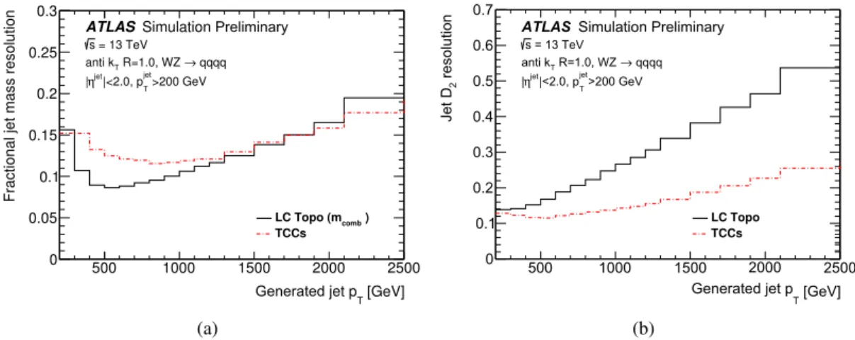
Figure 1 shows the striking improvement in D

resolutions4 achieved with TCC jets. The mass resolution is superior to previously used jet mass variables ( m

[64]) starting around a jet p

of 2 TeV. Below 1 TeV, the mass resolution in TCC jets is degraded. For identifying hadronically decaying V bosons, the improvement in D

resolution far outweighs the slight degradation in mass resolution.

5.3 Leptons

Electron identification is based on matching tracks to energy clusters in the electromagnetic calorimeter and calculating a likelihood based on several properties of the electron candidate. Electrons are required to have p

> 25 GeV and |η | < 2 . 5, and to satisfy the ‘medium’ identification criterion [65] and the ‘loose’

track-based isolation [65].

Muon identification relies on matching tracks in the inner detector to muon spectrometer tracks or track segments. Muons are required to have p

> 25 GeV and |η| < 2 . 5, and to satisfy the ‘loose’ selection criterion [66] and the ‘loose’ track isolation [66].

6 Event selection

To avoid contamination from non-collision backgrounds such as from calorimeter noise, beam halo, and cosmic rays, events containing an anti- k

jet built from calorimeter-cell clusters with R = 0 . 4 and

3

The angular exponent

, defined in Ref. [63], is set to unity.

4

The resolution is defined as

2

and

1

2

Q₇₅(R^d) −Q₂₅(R^d)

for the mass

and

, respectively, where

is the

is the median. The mass response is defined

as

, while the residual of

is

, where ‘gen’ and ‘reco’ refer to the generated and

reconstructed properties of the jets.

500 1000 1500 2500 [GeV]

T

0 0.05 0.1 0.15 0.2 0.25 0.3

Fractional jet mass resolution

LC Topo (m ) comb

TCCs ATLAS Simulation Preliminary

qqqq R=1.0, WZ → anti kT

>200 GeV

T

|<2.0, pjet

ηjet

| = 13 TeV s

Generated jet p 2000

(a)

500 1000 1500 2500

[GeV]

T

0 0.1 0.2 0.3 0.4 0.5 0.6 0.7

Jet D2 resolution

LC Topo TCCs qqqq

R=1.0, WZ → anti kT

>200 GeV

T

|<2.0, pjet

ηjet

| = 13 TeV s

Generated jet p 2000 ATLAS Simulation Preliminary

(b)

Figure 1: A comparison of (a) the fractional jet mass resolution for jets built from a linear combination of the calorimeter and track-only mass (LCTopo m

, solid line), and jets built using combined and neutral Track- CaloClusters objects (dashed lines) as a function of Monte Carlo generator-level jet p

. The fractional jet resolution of the D

variable (b) is compared between Track-CaloClusters and pure calorimeter jets. Only the two jets with the highest p

per event matched to a generated jet from a W or Z boson are shown.

p

> 20 GeV failing to meet the loose quality criteria for consistency with production in pp collisions are rejected [67]. In addition, events with at least one lepton meeting the requirements defined in Section 5.3 are rejected. There are no further requirements on leptons that are aligned with jets.

Events are required to have at least two anti- k

, R = 1 . 0, jets originating from the primary vertex, one with p

> 500 GeV and the second with p

> 200 GeV. The leading (highest p

) and subleading of these jets must satisfy |η | < 2 . 0 (to guarantee a good overlap with the tracking acceptance), have masses m

> 50 GeV, and their invariant mass, m

, must be larger than 1.3 TeV. The last requirement ensures that the triggers in use are fully efficient for the backgrounds and the benchmark signals. These selections are referred to as pre-selections.

The pair of jets is then required to have a small separation in rapidity, |∆ y

| < 1 . 2. This requirement reduces the multijet background, which is mainly produced in t -channel processes with large rapidity differences, in contrast to signal events that are expected to be produced in s -channel processes with small rapidity differences. Additionally, to reject events with potentially badly reconstructed jets, a criterion is applied to the p

asymmetry, A = (p

− p

) / (p

+ p

) < 0 . 15, where p

and p

are the transverse momenta of the leading and subleading jets, respectively.

6.1 Vector-boson identification

Jet substructure can be exploited to enhance the separation between signal boson jets and jets from multijet background. Several promising variables have been studied [62], with the largest sensitivity gain coming from the use of the three variables introduced in Section 5.2: jet mass, D

, and n

.

A three-dimensional (jet mass, D

, n

) tagger using TCC jets is optimised to provide maximum significance for boosted vector-boson jets relative to background jets. A measure of significance, independent of the cross-sections of the new processes being searched for, is selected: /(a/ 2 + √

B) , where is the

per-signal-jet selection efficiency for masses in the range of 0.5 TeV to 10 TeV in the W

model described

1 1.5 2 4 400.5

140 120 100 80 60 160 180

mJ[GeV]

2.5 3 3.5

Generated jet p ^[TeV]

T Z tagger

W tagger

ATLAS Simulation Preliminary s = 13 TeV

(a)

1 1.5 2 4

0.50.5 2

1.5

1 2.5 3 Jet D 2

2.5 3 3.5

Z tagger W tagger

Generated jet p ^[TeV]

T

ATLAS Simulation Preliminary s = 13 TeV

(b)

1 1.5 2 4

Generated jet p ^[TeV]

T

200.5 30 28 26 24 22 32

trkJet n

2.5 3 3.5

34

Z tagger W tagger

ATLAS Simulation Preliminary s = 13 TeV

(c)

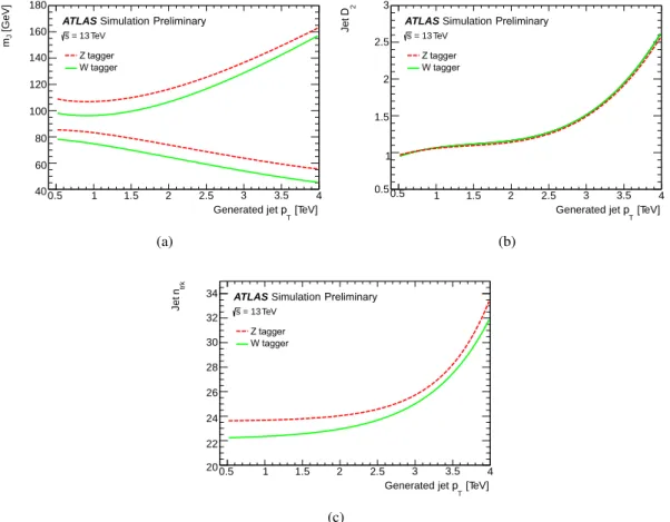
Figure 2: (a) Jet mass window, (b) D

selection and (c) n

selection of the W and Z taggers as a function of jet p

. Jets selected in the analysis are required to have jet masses inside the jet mass window and D

and n

values below the shown values. The tagger is only valid for jets with a p

between 0.5 TeV and 4.0 TeV and with |η

| < 2 . 0.

in Section 4.1, a is the number of standard deviations corresponding to a one-sided Gaussian distribution, and B is the number of background jets after the selection [68] taken from MC simulation. This number does not rely on a specific signal, but is valid for all signals with similar experimental features. Compared with the often used S/ √

B , that breaks down for small values of B , as is the case here, this measure is more appropriate. A value of a = 3 is used, where the result of the optimisation is not very sensitive to the exact value. For each jet p

bin, the optimal selection on the three variables is defined by the combination of selections that leads to the highest significance. This simultaneous treatment properly accounts for the correlations between the variables. The result of this optimisation does not depend on the pre-selections described at the beginning of this section. Next, the applied selection criteria on jet mass, D

, and n

are parameterised with jet- p

-dependent functions. For the jet mass, the function follows its approximate experimental resolution. For the latter two a simple higher-order polynomial is used. The resulting smooth selections for the W and Z boson taggers as a function of jet p

are shown in Figure 2. Jets selected in the analysis are required to have jet masses inside the jet mass window and D

and n

values below the shown values. It should be noted that the W and Z boson mass windows overlap. This search is not sensitive to signatures containing massive particles with masses different from W/Z boson masses (for example top quarks or Higgs bosons).

Unlike previous boson taggers [20], the optimisation described above does not enforce a fixed signal

0.5 1 1.5 2 2.5 3 3.5 4 [TeV]

Jet pT

0 0.2 0.4 0.6 0.8 1 1.2 1.4

W-tagging efficiency

s=13 TeV Mass efficiency cut

D2 efficiency cut nTrk efficiency cut Total efficiency ATLAS Simulation Preliminary

(a)

0.5 1 1.5 2 2.5 3 3.5 4

[TeV]

0 100 200 300 400 500 600 700 800 900 1000

Background rejection

Jet p [TeV]_T W tagger Pythia QCD Multijet s=13 TeV

ATLAS Simulation Preliminary

(b)

0.5 1 1.5 2 2.5 3 3.5 4

0 0.2 0.4 0.6 0.8 1 1.2 1.4

Z-tagging efficiency

=13 TeV s

[TeV]

Jet p ATLAS Simulation

T Mass efficiency cut D2 efficiency cut nTrk efficiency cut Total efficiency Preliminary

(c)

0.5 1 1.5 2 2.5 3 3.5 4

[TeV]

0 100 200 300 400 500 600 700 800 900 1000

Background rejection

Jet p [TeV]_T Z tagger Pythia QCD Multijet s=13 TeV

ATLAS Simulation Preliminary

(d)

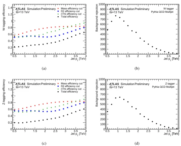
Figure 3: The (a) per-boson signal efficiency for the jet mass, D

, and n

selections, as well as the combined efficiency and (b) background rejection (1 / efficiency) of the W tagger for HVT W

→ W Z → qqqq and MC simulated multijets as a function of the jet p

. Corresponding values for the Z tagger are shown in (c) and (d).

efficiency nor a fixed background rejection, but rather creates a smooth behaviour that maximises the analysis sensitivity. Figure 3 shows the resulting W and Z boson efficiencies and multijet background rejections (defined as 1 / efficiency) as a function of jet p

. The selection criteria retain about 20% efficiency for W and Z boson jets with p

= 0 . 5 TeV. At higher jet p

, the signal efficiency increases, reaching an efficiency close to 60% for jets with a p

of 4 TeV. This is due to the behaviour of the multijet background, which decreases rapidly for high dijet masses, and thus higher jet p

. In the regime of m

> 3 . 0 TeV, where the number of background events is small, the tagger maintains a reasonable acceptance for signals with small cross-sections. This is also reflected in the background rejection as a function of jet p

. 6.2 Measurement of boson-tagging efficiency

The modelling of the boson-tagging efficiency is evaluated in a data sample enriched in final states with

a vector boson plus jets. This sample is obtained by requiring two large-radius jets with |η| < 2 . 0 and

then requiring that the leading jet has p

> 600 GeV. A higher minimum p

requirement is imposed on

the leading jet than in the nominal event selection to obtain a sample with higher average leading jet p

that better corresponds to the jet p

values probed in the search. Events with identified leptons are vetoed.

Both jets are independently analysed for the presence of a vector boson by requiring them to satisfy the D

and n

selection for either a W or a Z boson. The opposite jet is required to not satisfy the same D

selection to guarantee independence of this control region from the main analysis signal region.

The mass distribution of the selected jets between 50 GeV and 200 GeV is fit by a signal-plus-background function, allowing the inclusive rate of V + jets events to be measured. The contribution originating from V + jets processes is modelled using a double-Gaussian distribution with the shape parameters determined from simulation, while the background contribution is fit to data using a fourth-order exponentiated polynomial. The ability of the fit to extract the correct V + jets yield (also called MC closure) is tested in simulation by injecting signals of various strengths. Good linearity is found and the method is deemed reliable. By comparing the measured event yield in data and MC simulation, potential differences in the selection efficiency ( s

) can be probed. Expected contributions of about 5% from tt events are subtracted based on MC simulation. The cross-section of V + jets at a V p

of about 600 GeV is modelled with about 10% accuracy by the simulation [69]. Additional systematic uncertainties in the fitted V + jets event yield from closure, from the uncertainty in the tt contribution, as well as from the fit parameterisation are considered. The relative efficiency of the D

and n

selections is extracted for V bosons with p

starting from 600 GeV, while the analysis extends to p

= 3 . 5 TeV. To estimate the dependence of the modelling on the jet p

, the distribution of the D

and n

variables is compared in an inclusive sample in data and MC simulation as a function of jet p

. The observed residual mismodelling as a function of jet p

is taken into account as an additional 5% uncertainty in the relative efficiency.

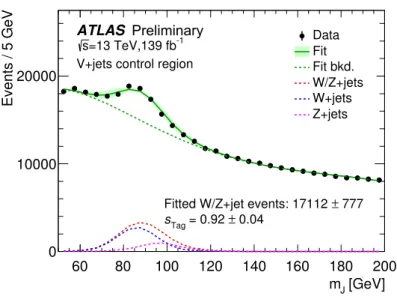
The fit to data is shown in Figure 4. This fit only extracts the overall yield, while the width and mean of the W/Z peaks are fixed from similar fits performed on MC simulation. The fitted relative efficiency of the D

and n

selections in data compared with MC simulation is s

= 0 . 92 ± 0 . 04 ( stat ) ± 0 . 02 ( closure ) ± 0 . 03 (tt) ± 0 . 02 ( fit ) ± 0 . 05 (p

range ) ± 0 . 10 ( theory ) , or s

= 0 . 92 ± 0 . 13. This is applied as a scale-factor to the signal MC events, where the uncertainty in it reflects the uncertainty in the W/Z -tagging efficiency in the simulation. Additional fits allowing both the width and the mean of the W/Z peaks to float are used to compare the efficiency of the jet mass window of the boson taggers in data and simulation. Excellent agreement is found, and no additional uncertainty is assigned. The polarisation of the vector bosons in this control region will be different from those in different signal models, but as no other physics process has sufficient sensitivity to probe the data-to-simulation agreement it is assumed that the simulation models the polarisation effects sufficiently well that the scale-factors can be applied globally.

6.3 Signal and background selection efficiency

After boson tagging, the data is categorised into three non-exclusive signal regions (SRs): events with two jets identified as WW , Z Z , or W Z each form a SR. Only the boson-tagging requirement differs between the regions. The highest mass jet of the two highest p

jets is considered as the candidate for the higher boson mass requirement. For the W Z selection this means that the highest mass jet must satisfy the Z boson selections and the second highest one the W boson selections. The selection requirements are summarised in Table 1.

The selection efficiency, defined as the number of selected events at different stages of the selection divided

by the number of generated events, as a function of the resonance mass, is shown in Figure 5 for the HVT

Z

decaying into WW and for the bulk G

decaying into Z Z . Similar efficiencies are obtained in the W Z

final state for the HVT model and in the WW final state for the bulk RS models. The figure shows that,

among the different selection criteria described above, the boson tagging reduces the signal efficiency the

60 80 100 120 140 160 180 200 [GeV]

m

0 10000 20000

Events / 5 GeV

Data Fit Fit bkd.

W/Z+jets W+jets Z+jets

ATLAS

s=13 TeV,139 fb^-1 V+jets control region

Tag

Fitted W/Z+jet events: 17112± 777 s = 0.92 ± 0.04

Preliminary

Figure 4: Jet mass distribution for data in the region enhanced in V + jets events after boson tagging based only on the D

and n

variables. The result of fitting to the sum of functions for the V + jets and background events is also shown. The shown fit uncertainty reflects the uncertainty in shape and positions of the W and Z peaks. At the bottom, the fitted contribution to the observed jet mass spectra from the V + jets signal is shown. The fitted relative efficiency of the D

and n

selections is s

= 0 . 92 ± 0 . 04, where the uncertainty is purely statistical.

Table 1: Event selection requirements and definition of the different regions used in the analysis. Different requirements are indicated for the highest- p

(leading) jet with index 1 and the second highest- p

(subleading) jet with index 2.

Signal region Veto events with leptons:

No e or µ with p

> 25 GeV and |η| < 2 . 5 Event pre-selection:

≥ 2 large- R jets with |η| < 2 . 0 and mass > 50 GeV p

> 500 GeV and p

> 200 GeV

m

> 1 . 3 TeV Topology and boson tag:

|∆ y | = | y

− y

| < 1 . 2

A = (p

− p

) / (p

+ p

) < 0 . 15

Boson tag with D

variable, n

variable, and W or Z mass window V +jets control region Veto events with leptons:

No e or µ with p

> 25 GeV and |η| < 2 . 5 V +jets selection:

≥ 2 large- R jets with |η| < 2 . 0 p

> 600 GeV and p

> 200 GeV

Boson tag with D

and n

variables on either jet

Anti-boson tag with D

variable on other jet

most. However, this particular selection also provides the most significant suppression of the dominant multijet background. The resulting width of the m

distributions in the signal region for a HVT model A W

→ W Z (Bulk RS graviton → Z Z ) is about 6% (10%) of its mean value across the mass range studied, corresponding to about 120 GeV (200 GeV) at 2 TeV. Multijet background events are suppressed with a rejection factor greater than 10

across the entire m

search range, as determined from simulation.

1.5 2 2.5 3 3.5 4 4.5 5

0 0.2 0.4 0.6 0.8 1 1.2

1.4 Pre-Selection

y|<1.2

|∆ A < 0.15 Mass cut

2 cut Dtrk cut n ATLASSimulation

s = 13 TeV HVT Z’ → WW

m(Z') [TeV]

Acceptance × Efficiency

Preliminary

(a)

1.5 2 2.5 3 3.5 4 4.5 5

0 0.2 0.4 0.6 0.8 1 1.2

1.4 Pre-Selection

y|<1.2

|∆ A < 0.15 Mass cut

2 cut Dtrk cut n

Acceptance × Efficiency ^KK

ATLASSimulation s = 13 TeV G → ZZ

) [TeV]

m(GKK

Preliminary

(b)

Figure 5: The acceptance × efficiency for the selection, defined as the number of selected events at different stages of the selection divided by the number of generated events, for (a) HVT Z

→ WW and (b) G

→ Z Z as a function of mass. The selections are applied in sequence and include pre-selections, topological selections on |∆y

| , p

asymmetry A , and boson tagging using jet mass, D

, and n

.

7 Background parameterisation

The search for diboson resonances is performed by looking for narrow peaks above the smoothly falling m

distribution expected from the SM. The background in the search is estimated empirically from the observed m

spectrum in the signal region. The background estimation procedure is based on a binned maximum-likelihood fit of the following parameterised form to the observed m

spectrum:

d n

d x = p

( 1 − x)

x

(1)

where x = m

/ √

s , p

is a normalisation factor, p

and p

are dimensionless shape parameters, and ξ is a constant. The value of ξ is derived in an iterative way, minimising the correlation between p

and p

in the fit, for each m

distribution. It is confirmed that the complexity of this fit function is sufficient for the expected number of events in the signal regions by performing Wilks likelihood-ratio tests [70]. The fit is performed to the m

distribution in each signal region in data with a constant bin size of 100 GeV. This choice is motivated by the experimental resolution.

The modelling of the parametric shape in Eq (1) is tested in dedicated fit control regions (CRs) in data.

These CRs are designed to resemble the expected background in the SRs in both their shape and number of

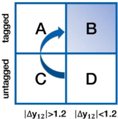
events, assuming that no signal contribution is present. Four regions are defined as shown in Figure 6,

where A and B differ for each tested SR. A possible contamination in region A, C, or D from a potential

beyond-the-SM signal is negligible. Region B corresponds to the nominal signal regions.

Figure 6: Four orthogonal regions used to build the fit control region for each signal region. A: |∆y

| > 1 . 2 with both the jets boson-tagged, B: |∆y

| < 1 . 2 with both the jets boson-tagged (this is the nominal signal region), C:

|∆y

| > 1 . 2 with the event not boson-tagged, D: |∆y

| < 1 . 2 with the event not boson-tagged. Regions A and C are used to derive a per-event transfer factor from region D to the fit control region, which is representative of region B.

A and C are also signal-depleted due to the |∆y

| > 1 . 2 requirement.

The probability of misidentifying either the highest or second highest mass jet in an event as a W or Z boson in a data sample dominated by multijets is parameterised as a function of jet p

using regions C and A. It is validated on data that such a probability is independent of |∆ y

| . Since a misidentification correlation between the two leading jets of the multijet background is observed after the pre-selections, the probability of the second highest mass jet is derived by requiring the highest mass jet to be in the mass window of the boson tagger. By applying per-jet weights, for the inverted selections, depending on the jet p

, events of the region D are transformed to resemble region B – the fit CRs. To correctly take into account the expected statistical fluctuations and uncertainties, the CR distributions are assigned the correct Poisson errors, and fluctuated accordingly. The last step is repeated multiple times, fitting each distribution with the background fit function, and evaluating the goodness-of-fit χ

/ NDF. Bins with fewer than five events are combined with bins that contain at least five events to compute the number of degrees of freedom (NDF). On average, the χ

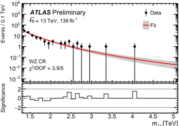
/ NDF is equal to unity with no cases for which the fit fails. Figure 7 shows the fit result performed in an example W Z fit CR. Similar results are obtained for the other CRs, confirming the ability of the chosen background fit function (Eq. (1)) to describe the expected background dijet mass spectra in the SRs. It is validated on both the data and the simulation that this parametric background description is valid up to 8.0 TeV, which is also the mass up to which the observed m

spectra are fit.

The statistical uncertainty in the background expectation comes directly from the uncertainty in the fitted

parameters of the background function, which assumes a smoothly falling m

distribution. Possible

additional uncertainties due to the background model are assessed by considering signal-plus-background

fits (also called spurious signal tests) of the chosen function to the fit control regions of data in which a

signal contribution is expected to be negligible. The background is modelled with Eq. (1) and the signal

is modelled using resonance mass distributions from simulation. These procedures were estimated to

introduce a bias smaller than 25% of the statistical uncertainty in the background estimate at any mass in

the search region, and no additional uncertainty is assigned.

1500 2000 2500 3000 3500 4000 4500 5000

Events / 0.1 TeV

−3

10

−2

10

−1

10 1 10 102

103

104

Data Fit ATLAS

s = 13 TeV, 139 fb^-1

WZ CR /DOF = 3.9/5 χ2

[TeV]

mJJ

1.5 2 2.5 3 3.5 4 4.5 5

Significance 2−

0 2

Preliminary

Figure 7: Comparison between fitted background shape and the m

spectra in an example W Z fit control region in data. The fitted background distribution is normalised to the data shown in the displayed mass range. The shaded bands represent the uncertainty in the background expectation calculated from the maximum-likelihood function.

The lower panel shows the significance, defined as the z -value as described in Ref. [71].

8 Systematic uncertainties

The uncertainties affecting the background modelling are taken directly from the errors in the fit parameters of the background estimation procedure described in Section 7. The systematic uncertainties in the expected signal yield and shapes arise from detector effects and MC modelling and are assessed and expressed in terms of nuisance parameters in the statistical analysis as described in Section 9.2. The dominant sources of uncertainty in the signal modelling arise from uncertainties in the large- R jet tagging efficiency and the jet p

calibration. These two uncertainties, and the uncertainty in the fitted background, are also the only ones significantly affecting the statistical results.

The uncertainty in the jet p

scale (J p

S) is evaluated using track-to-calorimeter double ratios between data and simulation [72]. The ratio of the calorimeter and track measures of jet p

is expected to be the same in data and simulation and any observed differences are assigned as baseline systematic uncertainties.

Uncertainties obtained from this procedure assume no correlation between the two p

measures, while any residual correlation would modify them by a certain factor. An upper limit to the correlation between the two p

measures is found to be at the percent level by comparing the results of this double-ratio procedure between jets built from TCC inputs and jets built from calorimeter-only inputs. Additional uncertainties due to the track reconstruction efficiency, track impact parameter resolution, and track fake rate are taken into account. The size of the total J p

S uncertainty varies with jet p

and is between 2 . 5% and 5% for the full mass range.

The impact of the jet p

resolution uncertainty is evaluated event-by-event by rerunning the analysis with an additional Gaussian smearing applied to the input jets’ p

to degrade the nominal resolution by the systematic uncertainty value. The systematic uncertainty in the width of the Gaussian distribution is an absolute 2% per jet, and is symmetrised.

Uncertainty in the jet mass scale and resolution influences the observed jet mass, affecting the boson-tagging

efficiency. Any uncertainty in the value of the boson-tagging discriminant D

or n

, would also affect

the selection efficiency of the analysis. A scale-factor for the W/Z -tagging efficiency is derived as

described in Section 6.2. The changes to the overall yield is hence corrected by 0 . 85

per event with the boson-tagging efficiency scale-factor, assuming full correlation between the two jets. The uncertainty in the scale-factor is assigned as a two-sided variation in the yield. Additional studies comparing jet properties in data and simulation confirm this uncertainty to be valid up to 7.0 TeV.

The uncertainty in the combined 2015–2018 integrated luminosity is 1.7%. It is derived from the calibration of the luminosity scale using x – y beam-separation scans, following a methodology similar to that detailed in Ref. [73], and using the LUCID-2 detector for the baseline luminosity measurements [74]. The uncertainty from the trigger selection is found to be negligible, as the minimum requirement on the dijet invariant mass of 1.3 TeV guarantees that the trigger is fully efficient.

Uncertainties in the behaviour of the PDFs at high Q

values can potentially have a large effect on the signal acceptance. This systematic uncertainty is estimated by taking the envelope formed by the largest deviations produced by the errors of three PDF sets, as set out by the PDF4LHC group [75]. A constant 1% uncertainty is applied in the case of the RS and radion models, and a pole-mass-dependent uncertainty ranging from 1%–12% is applied in the case of the HVT model. Systematic variations are used to cover uncertainties in the A14 tuned parameter values describing initial-state radiation, final-state radiation, and multi-parton interactions. The uncertainty in the signal acceptance is evaluated at the generator level, before boson-tagging requirements. Following the same procedure as for the PDFs, constant uncertainties of 3% (5%) are applied for the HVT (RS and radion) models.

9 Results

9.1 Background fit

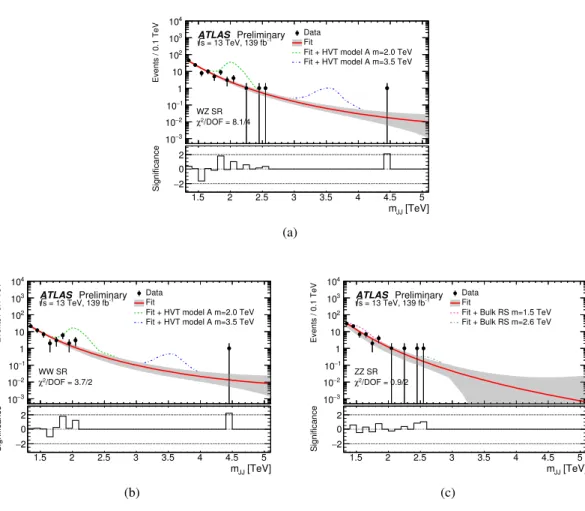
Figure 8 shows the comparison of the dijet mass distributions of the selected events in the W Z , WW , and Z Z signal regions with the expected background distribution from the background-only fits to the data.

The fitted background functions shown, labelled ‘Fit’, are evaluated in bins between 1.3 TeV and 8.0 TeV.

No events are observed beyond 5.0 TeV. A total of 57, 112, and 75 events are observed above 1 . 3 TeV in the W Z , WW , and Z Z signal regions, respectively. Due to the non-exclusive selections of the boson taggers, about 50% of events satisfying the WW selection also satisfy the Z Z selection. The highest mass event at 4.4 TeV is the same for both the W Z and WW signal regions, and it is compatible with the background expectation in the high mass region.

9.2 Statistical analysis

In the statistical analysis, the parameter of interest is the signal strength , which is defined as a scale-factor to the predicted signal normalisation of the model being tested. The analysis follows the frequentist approach with a test statistic based on the profile-likelihood ratio [76]. The test statistic extracts information about the signal strength from the binned maximum-likelihood fit of the signal-plus-background model to the data. The likelihood model is defined as,

L = Ö

i

P

(n

obs

|n

exp

) × G(α) × N (θ)

Events / 0.1 TeV

3

10− 2

10− 1

10−

1 10 102

103

104

Data Fit

Fit + HVT model A m=2.0 TeV Fit + HVT model A m=3.5 TeV ATLAS Preliminary _-1

= 13 TeV, 139 fb s

WZ SR /DOF = 8.1/4 χ2

[TeV]

mJJ

1.5 2 2.5 3 3.5 4 4.5 5

Significance 2−

0 2

(a)

Events / 0.1 TeV

3

10− 2

10− 1

10−

1 10 102

103

104

Data Fit

Fit + HVT model A m=2.0 TeV Fit + HVT model A m=3.5 TeV ATLAS Preliminary _-1

= 13 TeV, 139 fb s

WW SR /DOF = 3.7/2 χ2

[TeV]

mJJ

1.5 2 2.5 3 3.5 4 4.5 5

Significance 2−

0 2

(b)

Events / 0.1 TeV

3

10− 2

10− 1

10−

1 10 102

103

104

Data Fit

Fit + Bulk RS m=1.5 TeV Fit + Bulk RS m=2.6 TeV ATLAS Preliminary _-1

= 13 TeV, 139 fb s

ZZ SR /DOF = 0.9/2 χ2

[TeV]

mJJ

1.5 2 2.5 3 3.5 4 4.5 5

Significance 2−

0 2

(c)

Figure 8: Background-only fits to the dijet mass ( m

) distributions in data after tagging in the (a) W Z , (b) WW , and (c) Z Z signal region. The shaded bands represent the uncertainty in the background expectation calculated from the maximum-likelihood function. The lower panels show the significance, defined as the z -value as described in Ref. [71]. Selected theoretical signal distributions are overlaid on top of the background.

where P

(n

obs

|n

exp

) is the Poisson probability to observe n

obs

events if n

events are expected, G(α) are a series of Gaussian probability density functions modelling the systematic uncertainties, α , related to the shape of the signal, and N (θ) is a log-normal distribution for the nuisance parameters, θ , modelling the systematic uncertainty in the signal normalisation. The expected number of events is the bin-wise sum of those expected for the signal and background: n

= n

+ n

. The expected number of background events in dijet mass bin i , n

bg

, is obtained by integrating d n/ d x obtained from Eq. (1) over that bin. Thus n

is a function of the dijet background parameters p

, p

and p

. The expected number of signal events, n

, is evaluated from MC simulation assuming the cross-section of the model under test multiplied by the signal strength, including the effects of the systematic uncertainties described in Section 8.

The significance of observed excesses over the background-only prediction is quantified using the local p

-value, defined as the probability of the background-only model to produce a signal-like fluctuation at least as large as that observed in the data. The most extreme p

has a local significance of 1.8 standard deviations, and is found when testing the HVT W

→ WW hypothesis at a resonance mass of 1 . 8 TeV.

This is within the expected fluctuation of the background.

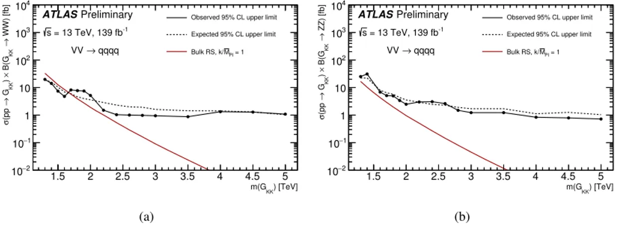
Limits at 95% confidence level (CL) on the production cross-section times branching fraction to diboson final states for the benchmark signals are set with sampling distributions generated using pseudo-experiments.

All systematic uncertainties are considered. The uncertainty in the W /Z -tagging efficiency is dominant at lower masses, while the uncertainty in the background modelling has largest impact at high masses.

Uncertainties in the jet p

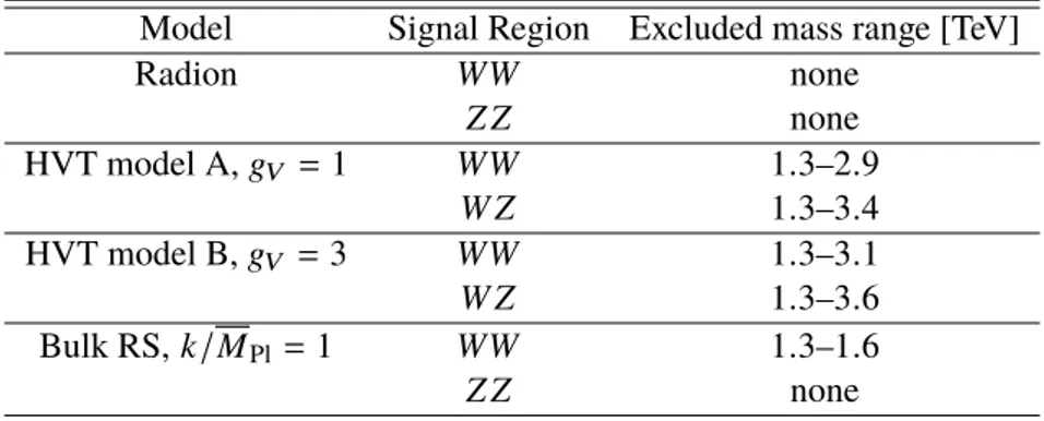
scale are at the percent level but are subordinate across the full mass range. The cross-section limits extracted for the different benchmark scenarios are shown in Figure 9, Figure 10 and Table 2. Table 3 presents the resonance mass ranges excluded at the 95% CL in the various signal regions and signal models considered in the search.

m(Z’) [TeV]

1.5 2 2.5 3 3.5 4 4.5 5

WW) [fb]→ B(Z’ × Z’) →(pp σ

2

10− 1

10−

1 10 102

103

104

10 10 1 10 10 10 ATLAS Preliminary 10

= 13 TeV, 139 fb-1

s

qqqq VV →

Observed 95% CL upper limit Expected 95% CL upper limit

V = 1 HVT model A, g

V = 3 HVT model B, g

(a)

m(W’) [TeV]

1.5 2 2.5 3 3.5 4 4.5 5

WZ) [fb]→ B(W’ × W’) →(pp σ

2

10− 1

10−

1 10 102

103

104

10 10 1 10 10 10 ATLAS Preliminary 10

= 13 TeV, 139 fb-1

s

qqqq VV →

Observed 95% CL upper limit Expected 95% CL upper limit

V = 1 HVT model A, g

V = 3 HVT model B, g

(b)

Figure 9: Observed and expected limits at 95% CL on the cross-section times branching ratio for WW production as function of (a) m

, and for W Z production as a function of (b) m

. The predicted cross-section times branching ratio is shown as dashed and solid lines for the HVT models A with g

= 1 and B with g

= 3, respectively.

) [TeV]

m(GKK

1.5 2 2.5 3 3.5 4 4.5 5

WW) [fb]→KK B(G×) KK G→(pp σ

2

10− 1

10−

1 10 102

103

104

10 10 1 10 10 10 ATLAS Preliminary 10

= 13 TeV, 139 fb-1

s

qqqq VV →

Observed 95% CL upper limit Expected 95% CL upper limit

PI = 1 M Bulk RS, k/

(a)

) [TeV]

m(GKK

1.5 2 2.5 3 3.5 4 4.5 5

ZZ) [fb]→KK B(G×) KK G→(pp σ

2

10− 1

10−

1 10 102

103

104

10 10 1 10 10 10 ATLAS Preliminary 10

= 13 TeV, 139 fb-1

s

qqqq VV →

Observed 95% CL upper limit Expected 95% CL upper limit

PI = 1 M Bulk RS, k/

(b)

Figure 10: Observed and expected limits at 95% CL on the cross-section times branching ratio for (a) WW and (b)

Z Z production as function of the Bulk RS graviton m

( k/M

= 1). The predicted cross-section times branching

ratio is shown as a solid line for the bulk RS model with k/M

= 1.

Table 2: Observed and expected limits at 95% CL on cross-section times branching ratio for WW and Z Z production for different radion masses m

, as well as the predicted cross-section times branching ratio.

Mass [TeV] Observed Limit [fb] Expected Limit [fb] Prediction [fb]

WW SR

2.0 5.35 3 . 60 2.755

3.0 1.46 2 . 20 0.267

4.0 1.61 1 . 91 0.026

5.0 1.58 1 . 69 0.004

ZZ SR

2.0 2.32 3 . 00 1.532

3.0 1.17 1 . 74 0.148

4.0 0.99 0 . 98 0.014

5.0 0.87 0 . 98 0.002

Table 3: Observed excluded resonance masses (at 95% CL) in the individual signal regions for the HVT, bulk RS and radion models.

Model Signal Region Excluded mass range [TeV]

Radion WW none

Z Z none

HVT model A, g

= 1 WW 1 . 3–2 . 9

W Z 1 . 3–3 . 4

HVT model B, g

= 3 WW 1 . 3–3 . 1

W Z 1 . 3–3 . 6

Bulk RS, k/M

= 1 WW 1 . 3–1 . 6

Z Z none

10 Conclusion

A search for narrow heavy resonances decaying into dibosons in the all hadronic channel is performed using 139 fb

of proton–proton collisions at

√ s = 13 TeV collected by the ATLAS experiment at the LHC from 2015 to 2018. The results of the search are shown for the WW , W Z , and Z Z channels, and are interpreted in terms of a radion model, two HVT benchmark models, and a bulk G

model. The data are in agreement with the background expectations in all channels. Upper limits on the production cross-section times branching ratio to diboson final states for new resonances with masses greater than 1.3 TeV are set at the 95% CL. These results exclude at the 95% CL the production of WW from the HVT model A (model B) with g

= 1 ( g

= 3) with masses in the range of 1.3 TeV–2.9 TeV (1.3 TeV–3.1 TeV).

The corresponding range for W Z production is 1.3 TeV–3.4 TeV (1.3 TeV–3.6 TeV). Production of WW from a G

in the bulk RS model with k /M

= 1 is excluded in the range 1.3 TeV–1.6 TeV, at the 95%

CL.