ATLAS-CONF-2012-081 07July2012
ATLAS NOTE
ATLAS-CONF-2012-081
July 2, 2012
Measurement of the flavour composition of dijet events in pp collisions at
√ s = 7 TeV with the ATLAS detector
The ATLAS Collaboration
Abstract
This note describes a measurement of the flavour composition of dijet events produced in pp collisions at
√s
=7 TeV using the ATLAS detector. The measurement uses the full 2010 data sample, corresponding to an integrated luminosity of 39 pb
−1. Six possible combinations of light, charm and beauty jets in the dijet events are identified, where the jet flavour is defined by the presence of beauty, charm or solely light flavour hadrons in the jet.
Kinematic variables, based on the properties of displaced decay vertices and optimized for jet flavour identification, are used in a multidimensional template fit to measure the fractions of these dijets flavour states as a function of the leading jet transverse momentum in the range 40 GeV to 500 GeV and jet rapidity
|y|<2.1. The fit results agree with the predictions of leading and next-to-leading order calculations, with the exception of the dijet fraction composed of beauty and light flavour jets, which is underestimated by all models at large transverse jet momenta. The ability to identify jets containing two b-hadrons, originated from e.g. gluon splitting, is demonstrated. The difference between beauty jet production rates in leading and subleading jets is consistent with the next-to-leading order prediction.
c Copyright 2012 CERN for the benefit of the ATLAS Collaboration.
Reproduction of this article or parts of it is allowed as specified in the CC-BY-3.0 license.
1 Introduction
A study of the production of jets containing beauty and charm hadrons and thus likely originating from beauty or charm quarks, is of strong interest for an understanding of Quantum Chromodynamics (QCD).
Charm and beauty quarks have masses significantly above the QCD scale,
ΛQCD, and hence their produc- tion can be calculated reliably using perturbation theory. They are thus excellent probes of the underlying QCD dynamics.
Several mechanisms contribute to heavy flavour quark production, such as quark-antiquark pair cre- ation in the hard interaction or in the parton showering process. While the former is calculable in a perturbative approach, the latter may require large non-perturbative c orrections or different approaches like a heavy quark mass expansion. In inclusive heavy flavour jet cross sections, the contributions from different heavy flavour quark production mechanisms are indistinguishable. This complicates a compar- ison with theoretical calculations. In contrast, a more exclusive study of the production of dijet events containing heavy flavour jets allows to separate the contributions of different heavy flavour quark cre- ation processes. For example, for beauty+beauty flavour jet pairs compared to beauty+light flavour jet pairs, the dominant QCD production mechanisms are different. In this context, a measurement of the flavour composition of dijet events sheds light on the details of the different QCD processes involving heavy quarks.
The dijet system can be decomposed into six flavour states based on the contributing jet flavours. The jet flavour is defined by the flavour of the heaviest hadron in the jet. A light jet originates from fragmenta- tion of a light flavour quark (u, d and s) or gluon and does not contain any beauty or charm hadron. Three of these dijet states are the symmetric beauty+beauty (b¯b), charm+charm (c¯c) and light+light jet pairs.
The three other combinations are the flavour-asymmetric beauty
+light, charm+light and beauty+charmjet pairs. In the following discussion, these six dijet flavour states will be denoted BB, CC, UU, BU, CU, BC, where U stands for light, C for charm and B for beauty jet.
Inclusive beauty jet and b¯b production in hadronic collisions has been studied by several experi- ments [1–6]. Recently CMS published cross sections for inclusive beauty jet production [7], b¯b decaying to muons [8] and beauty hadron production [9], as well as B ¯ B angular correlations [10]. The b¯b cross section was also measured by LHCb [11]. ATLAS published the measurement of the b¯b cross section in proton-proton collisions at
√s
=7 TeV [12], employing explicit b-jet identification (b-tagging). How- ever, the b¯b final state constitutes only a small fraction of the total heavy flavour quark production in dijet events, and the inclusive beauty cross section contains a significant contribution from multijet states. This note presents a simultaneous measurement of all six dijet flavour states, including those with charm. The BC, CC and CU dijet production at the LHC is studied for the first time. This approach provides more detailed information about the contributing QCD processes and challenges the theoretical description of the underlying dynamics employed in QCD Monte Carlo simulations.
The analysis procedure exploits reconstructed secondary vertices inside jets. Since kinematic proper- ties of secondary vertices depend on the jet flavour, a measurement of the individual contributions of each flavour can be made by employing a fit using templates of kinematic variables. No explicit b-tagging is used per se, i.e. no flavours are assigned to individual jets. The excellent separation of charm and beauty flavoured jets in the ATLAS detector is demonstrated in the analysis.
The analysis uses the data sample collected by ATLAS at
√s
=7 TeV in 2010, corresponding to an integrated luminosity of 39 pb
−1. The prescale settings of the different single jet triggers used in the analysis varied with luminosity such that the actual recorded luminosity is dependent on the transverse momentum p
Tof the leading jet.
This note is organized as follows. The ATLAS detector is briefly described in Section 2. Section 3
describes the event and jet selection procedure for data and Monte Carlo. Section 4 summarizes the
Monte Carlo simulation. Section 5 discusses the theoretical predictions for the flavour composition of
dijet events. The reconstruction of secondary vertices in jets as well as the kinematic templates for the flavour analysis are presented in Section 6. A detailed account of the analysis method is given in Section 7. In Section 8 the results of the analysis are presented and systematic uncertainties are discussed.
2 The ATLAS detector
The ATLAS detector [13] has been designed to allow the study of a wide range of physics processes at LHC energies. It consists of an inner tracking detector (ID), surrounded by an electromagnetic calorime- ter, hadronic calorimeters and a muon spectrometer. For the measurements presented in this paper, the tracking devices, the calorimeters and the trigger system are of particular importance.
The innermost detector, the tracker, is divided into three parts: the silicon pixel detector, the closest layer lying 5.05 cm from the beam axis, the silicon microstrip detector (SCT) and the transition radiation tracker (TRT), with the outermost layer situated at 1.07 m from the beam axis. These offer full coverage in the azimuthal angle
φand a coverage in pseudorapidity of
|η| <2.5
1. The tracker is surrounded by a solenoidal magnet of 2 T, which bends the trajectories of charged particles so that their transverse mo- menta can be measured. The liquid argon and lead electromagnetic calorimeter covers a pseudorapidity range of
|η|<3.2. It is surrounded by the hadron calorimeters, made of scintillating tiles and iron in the central region (
|η| <1.7) and of copper/tungsten and liquid argon in the endcaps (1.5
< |η| <3.2). A forward calorimeter extends the coverage to
|η| <4.9. The muon spectrometer comprises three layers of muon chambers for track measurements and trigger. It uses a toroidal magnetic field with a bending power of 1
−7.5 T.
The ATLAS trigger system [13] uses three consecutive levels: level 1 (L1), level 2 (L2) and event filter (EF). The L1 triggers are hardware-based and use coarse detector information to identify regions of interest, whereas the L2 triggers are based on fast online data reconstruction algorithms. Finally, the EF triggers use offline data reconstruction algorithms. This study uses ATLAS single jet triggers.
3 Event and jet selection
Selected events are required to have at least one reconstructed primary event vertex. The main interaction vertex must have at least 10 tracks with transverse momentum p
T >150 MeV associated to it, to ensure the quality of the vertex fit. If several vertices are reconstructed, the one with the largest sum of the squared transverse momenta of associated tracks is considered to be the main interaction vertex.
Jets are reconstructed using the anti-k
talgorithm with a jet resolution parameter R
=0.4 [14].
Topological calorimeter clusters are used as input for the clustering algorithm. Tracks within a cone of
∆R = p∆ϕ2+ ∆η2 =
0.4 around jet axis are assigned to the jet. Only jets with a transverse mo- mentum of p
T >30 GeV and a rapidity of
|y| <2.1 are considered. Jets in this rapidity range are fully contained in the tracker acceptance region, such that track and vertex reconstruction inside jets are not affected by the boundaries of the tracker acceptance. Jets are furthermore required to pass a quality se- lection [15] that removes jets coming from noisy calorimeter cells or those that stem from non-collision backgrounds. Finally, the two jets with highest p
Tin the analysis acceptance are required to have an angular separation in azimuth of
∆ϕ >2.1 rad, i.e. to be back-to-back. This cut removes events in which one of the leading jets is produced by final state hard gluon emission or jet splitting in the reconstruction.
The full data sample is split into six bins in the transverse momentum p
Tof the leading jet. The bin limits correspond to the 99 % efficiency working points of the various single jet triggers [16]. For
1ATLAS uses a right-handed coordinate system with its origin at the nominal interaction point (IP) in the centre of the detector and the z-axis along the beam pipe. The x-axis points from the IP to the centre of the LHC ring, and theyaxis points upward. Cylindrical coordinates (r, φ) are used in the transverse plane,φbeing the azimuthal angle around the beam pipe. The pseudorapidity is defined in terms of the polar angleθasη=−ln tan(θ/2).
Leading jet p
T[GeV] 40-60 60-80 80-120 120-160 160-250 250-500 Subleading jet p
T[GeV] 30-60 40-80 50-120 75-160 100-250 140-500 Number of events 304103 251406 887185 660168 242979 146117
R
Ldt [nb
−1] 70 247 1880 8640 8640 38700
Table 1: Kinematic boundaries, together with the numbers of selected dijet events and the corresponding integrated luminosities for each leading jet p
Tbin.
events passing the trigger requirement, the leading and subleading jets have to fulfil pairwise specific p
Tconditions that are summarized in Table 1. The numbers of events selected in each leading jet p
Tbin are shown in Table 1, together with the corresponding integrated luminosities.
4 Monte Carlo simulation
Dijet events are simulated using P
6.423 [17] for the baseline template construction, parameter estimation and Monte Carlo comparisons. This leading order (LO) generator is based on parton matrix element calculations for 2
→2 processes and a string hadronisation model. Modified leading order MRST LO* [18] parton distribution functions are used in the simulation. Samples of dijet events were generated using a specific set of generator parameters, known as the ATLAS Minimum Bias Tune 1 (AMBT1) [19].
For the study of systematic effects and for the interpretation of the final results, other Monte Carlo samples are utilised. The main cross-check study is performed using the H
++2.4.2 [20] genera- tor. The other LO samples used are P
with the next-to-leading order (NLO) CTEQ6.6 [21] parton distribution functions and H
6.5 [22] with the J
4 [23, 24] add-on for the simulation of mul- tiple parton interactions, using a specific ATLAS Underlying Event Tune (AUET1) [25]. The possible influence of multiple proton-proton interactions within the same bunch crossing is studied by adding minimum bias events, customized to the beam conditions of the 2010 LHC run at 7 TeV, to each P
event.
The P
6.423+E
G
[26] event generator, using exact charm and beauty decay tables, is utilised for the simulation of the physics of beauty hadron decays. It will be called P
+EG
in the rest of the note.
The NLO generator P
[27–30] is used to interpret the analysis results. In P
, the parton distribution function set used for the event generation is MSTW 2008 NLO [31] and the parton shower generator is P
.
In order to compare Monte Carlo predictions with data, truth particle jets are used. They are defined by the anti-k
tR
=0.4 algorithm using only stable particles with a lifetime longer than 10 ps in the Monte Carlo event record. Muons and neutrinos do not contribute significantly to the jet energy in data.
Therefore, they are also excluded from the truth particle jets, to avoid having to correct for the missing jet energy in data.
The flavour of jets is assigned in the Monte Carlo simulation by labelling a jet as a b-jet if a beauty hadron with p
T>5 GeV is found within a cone
∆R= p∆ϕ2+ ∆η2 =
0.3 around the jet axis. If no beauty hadron is present but a charm hadron is found using the same requirements, then the jet is labelled as a c-jet. All other jets are labelled as light jets. If two beauty hadrons with p
T >5 GeV are found within a cone of size
∆R=0.3 the jet is labelled as a b-jet with two beauty hadrons, and similarly for c-jets with two charm hadrons.
The particle four-momenta are passed through the full simulation [32] of the ATLAS detector, which
is based on G
4 [33]. The simulated events are reconstructed and selected using the same analysis
chain as for data. After the dijet event selection, the Monte Carlo events are reweighted in each analysis p
Tbin to match the observed leading and subleading jet p
Tspectra. Any remaining discrepancies in the rapidity distributions between data and simulation are small and are included as sources of systematic uncertainty, as detailed in Section 8.3.
5 Theoretical predictions
5.1 Heavy flavour production
Following the discussion in Ref. [34], heavy flavour quark production in hadronic collisions may be sub- divided into three classes depending on the number of heavy quarks participating in the hard scattering.
Hard scattering is defined as the 2
→2 subprocess with the largest virtuality (or shortest distance) in the hadron-hadron interaction. In the following, Q stands for a heavy flavour quark, q for a light flavour quark and
gfor a gluon.
•
Quark pair creation: two heavy quarks are produced in the hard subprocess. At leading order this is described by
gg→Q ¯ Q and q ¯q
→Q ¯ Q.
•
Heavy flavour quark excitation: a single heavy flavour quark from the sea of one hadron scatters against a parton from another hadron, denoted
gQ → gQ and qQ →qQ, respectively. Alterna- tively, the heavy flavour quark excitation process can be depicted as an initial state gluon splitting into a heavy quark pair, where one of the heavy quarks subsequently enters the hard subprocess.
•
Gluon splitting: in this case heavy quarks do not participate in the hard subprocess at all, but are produced in
g→Q ¯ Q branchings in the parton shower.
[GeV]
b-jet pT
30 100 200 1000
Production fraction
0 0.1 0.2 0.3 0.4 0.5 0.6 0.7 0.8 0.9 1
[GeV]
b-jet pT
30 100 200 1000
Production fraction
0 0.1 0.2 0.3 0.4 0.5 0.6 0.7 0.8 0.9 1
Quark pair creation Heavy flavour quark excitation Gluon splitting
Beauty production Pythia 6.423
ATLAS Preliminary Simulation
= 7 TeV s Truth jets,
(a)
[GeV]
b-jet pT
30 100 200 1000
Gluon splitting production fraction
0 0.1 0.2 0.3 0.4 0.5 0.6 0.7 0.8 0.9 1
[GeV]
b-jet pT
30 100 200 1000
Gluon splitting production fraction
0 0.1 0.2 0.3 0.4 0.5 0.6 0.7 0.8 0.9 1
Initial state gluon splitting Final state gluon splitting: jet with one b-hadron Final state gluon splitting:
jet with two b-hadrons
bb splitting
→ g
Pythia 6.423 ATLASPreliminary Simulation
= 7 TeV s Truth jets,
(b)
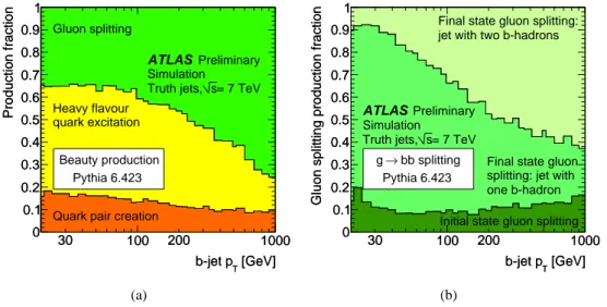
Figure 1: The contributions of the different production processes to inclusive b-jet production in 7 TeV
pp collisions are shown as a function of b-jet p
T, as given by P
6.423 and obtained for truth particle
jets. The plot on the left (a) shows the contribution of quark pair creation, heavy flavour quark excitation
and gluon splitting, the plot on the right (b) shows the different processes contributing to gluon splitting,
namely initial and final state gluon splitting, the latter leading to jets with one or two b-hadrons. Truth
particle jets are reconstructed with the anti-k
tR
=0.4 algorithm in the
|y|<2.1 rapidity region.
The relative contributions of the different heavy flavour quark production mechanisms to inclusive b- jet production are shown in Figure 1(a) for proton-proton collisions at 7 TeV. The fractions are calculated for anti-k
tjets in a rapidity range of
|y|<2.1 with the P
6.423 [17] generator. Figure 1(b) shows the decomposition of the gluon splitting process into initial and final state gluon splitting, the latter leading to jets with one or two b-hadrons.
The above classification is not strict but can be used as a basis for gaining a qualitative understanding of the features of heavy flavour quark production. Pair creation of heavy flavour quarks gives an insight into perturbative QCD with massive quarks. The back-to-back requirement used in the analysis reduces the contribution of NLO QCD effects to the jet-pair cross sections with two heavy flavour jets, BB and CC. The heavy flavour quark excitation process, on the other hand, is sensitive to the heavy flavour components of the parton distribution functions of the proton. It produces mainly flavour asymmetric BU and CU jet pairs. The gluon splitting mechanism is sensitive to non-perturbative QCD dynamics and also contributes significantly to the mixed flavour jet pair states, i.e. BU and CU. However, this contribution is different from heavy flavour quark excitation because it creates a heavy quark-antiquark pair that is practically collinear. Therefore the jet reconstruction algorithm either includes both heavy quarks in a single jet or misses one of them, thus reducing the reconstructed jet energy and its fraction taken by the remaining quark. The two possibilities result in different kinematic properties of the reconstructed secondary vertices in these jets, which can be exploited for the separation of gluon splitting from the heavy flavour quark excitation contribution.
[GeV]
Leading jet pT
100 200 300 400 500
Fraction
10-2
10-1
1 ATLAS Preliminary Simulation, Pythia 6.423
= 7 TeV s Truth dijets,
CU BU CC BC BB
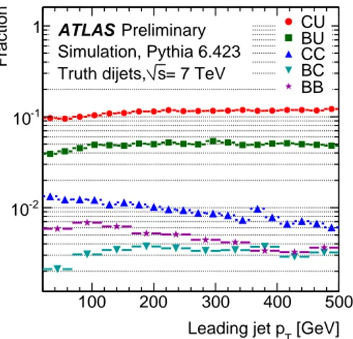
Figure 2: P
6.423 predictions for different beauty and charm dijet fractions as a function of leading jet p
T, obtained for truth particle jet pairs, where the jets are back-to-back and have p
T >20 GeV in the
|y|<
2.1 rapidity region.
To compare the predictions of theoretical models with data, the truth particle jets defined in Section 4 are used in the analysis. The truth particle dijet system is defined as the two truth particle jets with the highest p
Tin the
|y| <2.1 rapidity range, required to be back-to-back,
∆ϕ >2.1 rad, with leading and subleading jet having p
T >20 GeV.
The leading order predictions for flavour jet production in truth particle dijet events are illustrated
in Figure 2, where the ratio of different heavy+heavy and heavy+light dijet cross sections to the total
dijet cross section is shown for
|y| <2.1 as a function of leading jet p
T, for 7 TeV pp collisions as
predicted by P
6.423. Heavy flavour jets in the dijet system are mainly produced in the BU and CU
combinations. P
6.423 predicts a slow decrease of the BB and CC fractions and an increase of the
BU and CU jet fractions as a function of the leading jet p
T. The mixed BC fraction increases with jet p
Tand becomes equal to the BB fraction above
∼350 GeV.
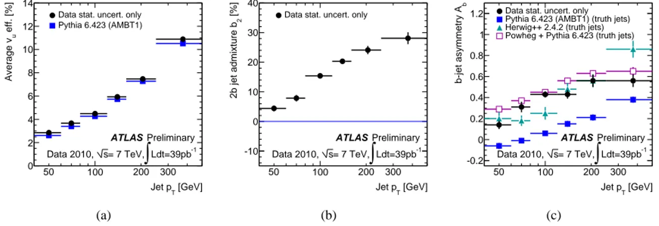
5.2 Di ff erences in heavy flavour rates in leading and subleading jets
[GeV]
Leading jet pT
50 100 200 300
bb-jet asymmetry A
-0.2 0 0.2 0.4 0.6 0.8 1 1.2 1.4
Powheg + Pythia 6.423 Pythia 6.423
Herwig++ 2.4.2 Pythia 6.423 + EvtGen
= 7 TeV s Truth dijets, ATLAS Preliminary Simulation
[GeV]
Leading jet pT
50 100 200 300
cc-jet asymmetry A
-0.2 -0.1 0 0.1 0.2 0.3 0.4 0.5 0.6
Powheg + Pythia 6.423 Pythia 6.423
Herwig++ 2.4.2 Pythia 6.423 + EvtGen
= 7 TeV s Truth dijets, ATLAS Preliminary Simulation
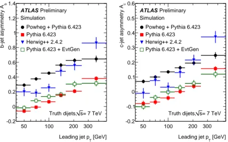
Figure 3: The asymmetries in the amount of beauty (left) and charm (right) truth particle jets as taken from P
+P6.423 (black points), P
6.423 (red squares), H
++2.4.2 (blue triangles) and P
+EG
(green squares) in leading and subleading jets, for each leading jet p
Tbin used in the analysis.
The kinematic properties of the partons produced in hadronic interactions are mostly flavour inde- pendent, if mass effects are neglected. Therefore the two back-to-back partons with the highest p
Tin the event should not demonstrate any significant flavour-dependent difference in their kinematic features.
However, the partons can be studied only through the corresponding jet properties after hadronization.
Heavy flavour quark presence in a jet can influence the jet properties through the following mechanisms:
•
Semileptonic decays of heavy flavour hadrons decrease the jet energy, because neutrinos are not detected and the muon energy is not measured in the calorimeter. This energy loss is absent for light jets and is very different for beauty and charm jets.
•
If several heavy flavour quarks appear in the jet fragmentation process (e.g. via gluon splitting) one of them can be left outside the jet volume by the jet reconstruction algorithm, which leads to a reduction in the jet energy.
As a result, the average jet energy for heavy flavours becomes smaller than the jet energy for light flavours, such that heavy flavour jets are predominantly produced as subleading jets in the mixed-flavour dijet pairs. This effect can be described using a flavour asymmetry defined as
A
b,c=N
b,cS LN
b,cL −1, (1)
where N
b,cL,S Ldenote the number of leading or subleading beauty or charm jets. The predictions for A
b,cgiven by different Monte Carlo generators are shown in Figure 3 for the truth particle je ts defined in
Section 5.1.
P
, which includes higher order QCD effects, predicts a significant flavour asymmetry which increases strongly with jet p
T. The predictions of the LO P
generator are smaller than those of the NLO P
generator. The latter uses P
6.423 for the fragmentation and thus shares the same description of the decays of heavy flavour hadrons. Since the influence of the different parton distribution functions was found to be negligible as well, the differences in A
b,cbetween these generators (Figure 3) should be attributed primarily to NLO QCD effects.
The LO H
++generator employs another fragmentation model and predicts asymmetries similar to the P
ones, although with a somewhat different p
Tdependence.
For the measurement of the dijet flavour fractions, this flavour asymmetry needs to be correctly described in the data analysis. The fact that the Monte Carlo generators predict significantly different asymmetries indicates that A
b,cshould be determined directly from the data.
6 Secondary vertex reconstruction and analysis templates
Secondary vertices are displaced from a primary interaction point because they originate from the decays of long-lived particles. Kinematic properties of these vertices, e.g. the invariant mass or total energy, depend on the corresponding properties of the original heavy flavour hadrons and are therefore different for beauty and charm jets. Reconstructed secondary vertices in light jets are mainly due to K
S0and
Λdecays [35], interactions in the detector material, or fake vertices. The fake reconstructed vertices are composed of tracks which occasionally become close due to large density of tracks in the jet core and track reconstruction errors. Their properties are very di
fferent from those of heavy flavour decays.The current analysis exploits these differences by combining the kinematic features of the reconstructed secondary vertices in an optimal way into templates for beauty, charm and light jets.
6.1 Secondary vertex reconstruction in jets
The vertex reconstruction algorithm aims at a high reconstruction efficiency and therefore determines vertices in an inclusive way, i.e. a single geometrical secondary vertex is fitted for each jet. In the case of a beauty hadron decay, the subsequent charm hadron decay vertex is usually close to the beauty one and is therefore not reconstructed separately. A detailed discussion of the algorithm and its performance can be found in the b-tagging chapter of [16]. The reconstruction starts by joining good quality tracks inside jets pairwise to vertices, where the latter are required to be displaced significantly from the primary interaction vertex. The two-track vertices coming from K
S0and
Λdecays and interactions in the detector material are removed from further consideration. For the light jets, the rema ining candidates after this cleaning are mainly fake vertices. All remaining two-track vertices are merged into a single vertex.
This vertex is refitted iteratively by removing tracks until a good vertex fit quality is obtained. The corresponding decay length is defined as a signed quantity, where the sign is fixed by the projection of the decay length vector - the vector pointing from the primary event vertex to the secondary vertex - on the jet axis. The vertex is required to have a positive decay length and a total invariant mass, calculated using the momenta of associated particles and assuming their pion masses [35], greater than 0.4 GeV.
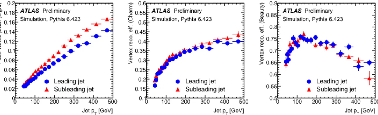
6.2 Secondary vertex reconstruction e ffi ciencies
The secondary vertex reconstruction efficiency is dependent on the jet p
T, due to several effects such as
the p
Tdependence of the track reconstruction accuracy and the increase of the flight distance of heavy
flavour hadrons with growing jet p
T. The probability of reconstructing a fake vertex in a light jet is
also affected by the increase of the number of tracks in a jet with jet p
T. Due to the p
Tdependent
vertex efficiency and different p
Tdistributions for leading and subleading jets in dijet pairs, a number of
reconstructed secondary vertices in these jets also become different.
[GeV]
Jet pT
0 100 200 300 400 500
Fake vertex prob. (Light)
0 0.02 0.04 0.06 0.08 0.1 0.12 0.14 0.16 0.18 0.2
ATLAS Preliminary Simulation, Pythia 6.423
Leading jet Subleading jet
[GeV]
Jet pT
0 100 200 300 400 500
Vertex reco. eff. (Charm)
0.1 0.15 0.2 0.25 0.3 0.35 0.4 0.45 0.5 0.55 0.6
ATLAS Preliminary Simulation, Pythia 6.423
Leading jet Subleading jet
[GeV]
Jet pT
0 100 200 300 400 500
Vertex reco. eff. (Beauty)
0.5 0.55 0.6 0.65 0.7 0.75 0.8 0.85 0.9
ATLAS Preliminary Simulation, Pythia 6.423
Leading jet Subleading jet
Figure 4: The reconstruction probabilities for fake vertices in light jets, as well as the reconstruction efficiencies for secondary vertices in beauty and charm jets, are displayed as a function of the jet p
Tas predicted by P
6.423.
The secondary vertex reconstruction efficiencies predicted by the ATLAS detector simulation based on dijet events from P
6.423 are shown in Figure 4. There is no difference between secondary vertex reconstruction efficiencies in leading and subleading jets for charm and beauty jets. However, the vertex reconstruction probability in light jets is noticeably bigger for subleading jets. This requires the introduction of two separate secondary vertex probabilities for leading and subleading light jets.
6.3 Template construction and features
The specific choice of the kinematic variables for the dijet flavour measurement is driven by the require- ment to have maximal sensitivity to the flavour content. Furthermore, if several variables are to be used, the correlations between them should be kept small. Another important requirement is a minimal depen- dence on the jet p
Tand rapidity, in order to minimize systematic effects due to a possible p
Tor rapidity mismatch between data and Monte Carlo. Also, p
T-invariant variables allow a robust analysis to be made over a wide range of p
T.
For this study the following two variables are chosen
Π =
M
vertex−0.4 GeV
M
B ·P
vertex
E
iP
jet
E
i(2)
B
=√
M
B· Pvertex|
p
Ti|M
vertex· rP
jet
E
Ti,
(3)
where each sum indicates whether the summation is performed over particles associated to the secondary vertex, or over all charged particles in the jet. Transverse momentum and energy are denoted as p
Tand E
T, respectively. In essence,
Πis the product of the invariant mass of the particles associated to the vertex (M
vertex) and the energy fraction of these particles with respect to all charged particles in the jet. The 0.4 GeV constant present in (2) is the cut value used for the secondary vertex selection in this analysis.
The parameter B corresponds approximately to the relativistic
γfactor of the system composed of the
particles associated to the vertex, normalized to the square root of the jet energy. The M
B=5.2794 GeV
constant is the average B-meson mass [35] and is used for normalization.
To reduce statistical fluctuations in regions with a small number of entries and to facilitate the fit procedure, the variables are transformed into the interval [0,1]:
Π⊤= Π
Π +
0.04 (4)
B
⊤=B
·B
B
·B
+10.
.(5)
The tuning constants 0.04 in (4) and 10 in (5) have been chosen such as to maximize the difference in the mean values between the light and heavy flavour distributions.
(Light) ΠΤ
0 0.1 0.2 0.3 0.4 0.5 0.6 0.7 0.8 0.9 1 (Light)ΤB
0 0.1 0.2 0.3 0.4 0.5 0.6 0.7 0.8 0.9 1
ATLAS Preliminary Simulation, Pythia 6.423
in [60,80] GeV Jet pT
(Charm) ΠΤ
0 0.1 0.2 0.3 0.4 0.5 0.6 0.7 0.8 0.9 1 (Charm)ΤB
0 0.1 0.2 0.3 0.4 0.5 0.6 0.7 0.8 0.9 1
(Beauty) ΠΤ
0 0.1 0.2 0.3 0.4 0.5 0.6 0.7 0.8 0.9 1 (Beauty)ΤB
0 0.1 0.2 0.3 0.4 0.5 0.6 0.7 0.8 0.9 1
Figure 5: Two-dimensional distributions of
Π⊤and B
⊤(flavour templates) obtained with P
6.423 for jets with p
Tin the [60, 80] GeV.
Joint distributions of these observables are shown in Figure 5 for light, charm and beauty jets in the [60, 80] GeV bin, as predicted by the full detector simulation of P
6.423 events. These two- dimensional distributions are used as flavour templates U(Π
⊤,B
⊤), C(Π
⊤,B
⊤) and B(Π
⊤,B
⊤) in the analysis as detailed in Section 7. Features of the observables are also illustrated in Figures 6, 7 and 8.
Both
Π⊤and B
⊤are independent of jet rapidity, as can be seen in Figure 6. This figure shows the light jet templates, which are most sensitive to reconstruction and detector effects. The
Π⊤variable is very similar in shape in the [40, 60] GeV and [250, 500] GeV bins and is only weakly p
Tdependent. Figures 7 and 8 demonstrate that the
Π⊤is only weakly dependent on the different heavy flavour production mechanisms described in Section 5. In contrast, the B
⊤variable is sensitive to the gluon splitting contribution, in particular to the case where this mechanism produces two quarks of the same flavour in a jet. In addition B
⊤has a distinct p
Tdependence. However, the B
⊤variable provides a good sensitivity to the charm contribution.
The fraction of jets with two heavy quarks produced in gluon splitting may be incorrectly predicted by the P
simulation, especially in the high p
Tregion where this contribution becomes large (see Figure 1). This phenomenon was discussed in more details in [36]. Therefore a separate contribution of doubly flavoured jets is included in the analysis, to cope with the corresponding dependence of the B
⊤variable. The two-dimensional template for beauty jets is replaced by the following two-component template
B(Π
⊤,B
⊤)
→(1
−b
2)
·B(Π
⊤,B
⊤)
+b
2·B
2(Π
⊤,B
⊤), (6)
where B
2(Π
⊤,B
⊤) is a template for jets with two b-hadrons and b
2is a parameter governing the rel-
ative contributions. The charm jet template is modified similarly with substitutions b
2 →c
2and
B
2(Π
⊤,B
⊤)
→C
2(Π
⊤,B
⊤). Using (6), the heavy flavour template shapes can be made “data driven”
ΠT
0 0.1 0.2 0.3 0.4 0.5 0.6 0.7 0.8 0.9 1
Fraction of entries / 0.04
0 0.05 0.1 0.15 0.2 0.25
0.3 |<0.5
0.0<|yjet
|<1.0 0.5<|yjet
|<1.5 1.0<|yjet
|<2.1 1.5<|yjet ATLAS Preliminary
Simulation, Pythia 6.423 u-jets
in [40,60] GeV LJ pT
BT
0 0.1 0.2 0.3 0.4 0.5 0.6 0.7 0.8 0.9 1
Fraction of entries / 0.04
0 0.02 0.04 0.06 0.08 0.1 0.12 0.14
0.16 |<0.5
0.0<|yjet
|<1.0 0.5<|yjet
|<1.5 1.0<|yjet
|<2.1 1.5<|yjet ATLAS Preliminary
Simulation, Pythia 6.423 u-jets
in [40,60] GeV LJ pT
(a) Light jets in [40,60] GeV
ΠT
0 0.1 0.2 0.3 0.4 0.5 0.6 0.7 0.8 0.9 1
Fraction of entries / 0.04
0 0.05 0.1 0.15 0.2 0.25
0.3 |<0.5
0.0<|yjet
|<1.0 0.5<|yjet
|<1.5 1.0<|yjet
|<2.1 1.5<|yjet ATLAS Preliminary
Simulation, Pythia 6.423 u-jets
in [250,500] GeV LJ pT
BT
0 0.1 0.2 0.3 0.4 0.5 0.6 0.7 0.8 0.9 1
Fraction of entries / 0.04
0 0.02 0.04 0.06 0.08 0.1 0.12
0.14 |<0.5
0.0<|yjet
|<1.0 0.5<|yjet
|<1.5 1.0<|yjet
|<2.1 1.5<|yjet ATLAS Preliminary
Simulation, Pythia 6.423 u-jets
in [250,500] GeV LJ pT
(b) Light jets in [250,500] GeV
Figure 6: The
Π⊤and B
⊤distributions of light jets in the [40, 60] GeV (a) and [250, 500] GeV (b) leading jet (LJ) p
Tanalysis bins obtained with fully simulated P
6.423 dijet events. The distributions are shown in different jet rapidity ranges.
by optimizing the b
2(c
2) parameters to obtain the best possible data description. As will be demon- strated in Section 8, the adjustment of the contribution of jets with two b-hadrons to the beauty template significantly improves the overall quality of the description of the dijet data.
6.4 Template tuning on data using track impact parameters
The secondary vertex reconstruction algorithm uses track impact parameters divided by their measure- ment uncertainties for the vertex search, thus its results depend crucially on the track impact parameter resolution. A good description of the track impact parameter accuracy and the corresponding covariance matrix is therefore mandatory in the detector simulation, in order for the secondary vertex templates to be constructed correctly.
To improve the agreement between data and Monte Carlo simulation, the analysis templates are tuned on data. Firstly, an additional track impact parameter smearing is applied to the P
events.
To estimate the necessary amount of smearing, the data and Monte Carlo track impact parameter dis-
ΠT
0 0.1 0.2 0.3 0.4 0.5 0.6 0.7 0.8 0.9 1
Fraction of entries / 0.04
0 0.02 0.04 0.06 0.08 0.1 0.12 0.14
Pair creation Flavour excitation
1c in jet
≥ GS, GS, 2c in jet ATLAS Preliminary
Simulation, Pythia 6.423 c-jets
in [40,60] GeV LJ pT
BT
0 0.1 0.2 0.3 0.4 0.5 0.6 0.7 0.8 0.9 1
Fraction of entries / 0.04
0 0.02 0.04 0.06 0.08 0.1 0.12 0.14
0.16 Pair creation
Flavour excitation 1c in jet
≥ GS, GS, 2c in jet ATLAS Preliminary
Simulation, Pythia 6.423 c-jets
in [40,60] GeV LJ pT
(a) Charm jets in [40,60] GeV
ΠT
0 0.1 0.2 0.3 0.4 0.5 0.6 0.7 0.8 0.9 1
Fraction of entries / 0.04
0 0.02 0.04 0.06 0.08 0.1 0.12
0.14 Pair creation
Flavour excitation 1c in jet
≥ GS, GS, 2c in jet ATLAS Preliminary
Simulation, Pythia 6.423 c-jets
in [250,500] GeV LJ pT
BT
0 0.1 0.2 0.3 0.4 0.5 0.6 0.7 0.8 0.9 1
Fraction of entries / 0.04
0 0.05 0.1 0.15 0.2 0.25
Pair creation Flavour excitation
1c in jet
≥ GS, GS, 2c in jet ATLAS Preliminary
Simulation, Pythia 6.423 c-jets
in [250,500] GeV LJ pT
(b) Charm jets in [250,500] GeV
Figure 7: The
Π⊤and B
⊤distributions for charm jets in the [40, 60] GeV leading jet (LJ) p
Trange (a) as well as in the [250, 500] GeV range (b) obtained with fully simulated P
6.423 dijet events.
The distributions are shown separately for jets stemming from quark pair creation, heavy flavour quark excitation, gluon splitting (GS) and the specific case of gluon splitting with two heavy flavour quarks inside the jet. All distributions are normalized separately to unit area.
tributions are compared in bins of track p
Tand pseudorapidity. However, the smearing procedure does
not correct the track covariance matrices and has a limited accuracy of the data description. Therefore,
a second step is made. Two sets of templates are produced, using both the smeared and non-smeared
P
6.423 samples. A normalized mixture is then compared with the data, using secondary vertices
with negative decay length to obtain the optimal mixing fraction. These vertices depend only weakly on
the exact flavour content of jets and are not used in the dijet analysis. The mixing fraction is chosen to be
flavour independent. The optimal description of the data for the full p
Trange is obtained with a fraction
F
smear=0.654
±0.023 for the smeared template in the mixture. This template tuning procedure gives a
significant improvement in the data fit quality in the signal region.
ΠT
0 0.1 0.2 0.3 0.4 0.5 0.6 0.7 0.8 0.9 1
Fraction of entries / 0.04
0 0.02 0.04 0.06 0.08 0.1 0.12 0.14 0.16 0.18
0.2 Pair creation
Flavour excitation 1b in jet
≥ GS, GS, 2b in jet ATLAS Preliminary
Simulation, Pythia 6.423 b-jets
in [40,60] GeV LJ pT
BT
0 0.1 0.2 0.3 0.4 0.5 0.6 0.7 0.8 0.9 1
Fraction of entries / 0.04
0 0.02 0.04 0.06 0.08 0.1 0.12 0.14 0.16 0.18 0.2
Pair creation Flavour excitation
1b in jet
≥ GS, GS, 2b in jet ATLAS Preliminary
Simulation, Pythia 6.423 b-jets
in [40,60] GeV LJ pT
(a) Beauty jets in [40,60] GeV
ΠT
0 0.1 0.2 0.3 0.4 0.5 0.6 0.7 0.8 0.9 1
Fraction of entries / 0.04
0 0.02 0.04 0.06 0.08 0.1 0.12 0.14 0.16
0.18 Pair creation
Flavour excitation 1b in jet
≥ GS, GS, 2b in jet ATLAS Preliminary
Simulation, Pythia 6.423 b-jets
in [250,500] GeV LJ pT
BT
0 0.1 0.2 0.3 0.4 0.5 0.6 0.7 0.8 0.9 1
Fraction of entries / 0.04
0 0.02 0.04 0.06 0.08 0.1 0.12 0.14 0.16 0.18
0.2 Pair creation
Flavour excitation 1b in jet
≥ GS, GS, 2b in jet ATLAS Preliminary
Simulation, Pythia 6.423 b-jets
in [250,500] GeV LJ pT
(b) Beauty jets in [250,500] GeV
Figure 8: The
Π⊤and B
⊤distributions for beauty jets in the [40, 60] GeV leading jet (LJ) p
Trange (a) as well as in the [250, 500] GeV range (b) obtained with fully simulated P
6.423 dijet events.
The distributions are shown separately for jets stemming from quark pair creation, heavy flavour quark excitation, gluon splitting (GS) and the specific case of gluon splitting with two heavy flavour quarks inside the jet. All distributions are normalized separately to unit area.
7 Analysis method
7.1 Dijet system description
The secondary vertex reconstruction procedure can find vertices with probabilities
vU,
vCand
vBfor
light, charm and beauty jets, respectively. For simplicity, the p
Tdependence of these probabilities and
the differences between leading and subleading jets (see Section 6.2) are neglected for the moment. In
the leading and subleading jet of a dijet event, zero, one or two secondary vertices can be reconstructed
overall. The numbers of 2-, 1-, or 0-vertex dijet events can be calculated as:
N
2VN
= vUvUf
UU+vCvCf
CC+vBvBf
BB(7)
+vUvCf
CU +vUvBf
BU+vCvBf
BCN
1VN
=2 (1
−vU)
vUf
UU+2 (1
−vC)
vCf
CC+2 (1
−vB)
vBf
BB(8)
+((1
−vU)v
C+vU(1
−vC)) f
CU+
((1
−vU)v
B+vU(1
−vB)) f
BU+
((1
−vC)v
B+vC(1
−vB)) f
BCN
0V=N
−N
1V−N
2V.(9)
Here N is the total number of dijet events, f
XXis the fraction of the respective dijet flavour component chosen such that
f
UU+f
CC+f
BB+f
CU+f
BU+f
BC =1. (10) The joint distribution of the
Π⊤and B
⊤variables for dijet events with one reconstructed secondary vertex can be obtained easily, using (8):
D
(Π
⊤,B
⊤)
=2 (1
−vU)
vUf
UUU(Π
⊤,B
⊤) (11)
+2 (1−vC)
vCf
CCC(Π
⊤,B
⊤)
+2 (1−vB
)
vBf
BBB(Π
⊤,B
⊤)
+(1
−vU)v
CC(Π
⊤,B
⊤)
+vU(1
−vC)U(Π
⊤,B
⊤) f
CU+
(1
−vU)v
BB(Π
⊤,B
⊤)
+vU(1
−vB)U(Π
⊤,B
⊤) f
BU+
(1
−vC)v
BB(Π
⊤,B
⊤)
+vC(1
−vB)C(Π
⊤,B
⊤) f
BC.Here
D(Π
⊤,B
⊤) is the observed data distribution and U(Π
⊤,B
⊤), C(Π
⊤,B
⊤) and B(Π
⊤,B
⊤) are templates derived from Monte Carlo with
Z
U(Π
⊤,B
⊤)dΠ
⊤dB
⊤ = ZC(Π
⊤,B
⊤)dΠ
⊤dB
⊤(12)
= Z
B(Π
⊤,B
⊤)dΠ
⊤dB
⊤=1.
The case of two reconstructed vertices requires more careful consideration. Assuming that the two jets are independent, the joint distribution of
Π⊤and B
⊤can be written considering (7) in the following way
D
(Π
⊤1,B
⊤1,Π⊤2,B
⊤2)
= +vUvUf
UU·U(Π
⊤1,B
⊤1)U(Π
⊤2,B
⊤2) (13)
+vCvCf
CC·C(Π
⊤1,B
⊤1)C(Π
⊤2,B
⊤2)
+vBvB
![Figure 5: Two-dimensional distributions of Π ⊤ and B ⊤ (flavour templates) obtained with P 6.423 for jets with p T in the [60, 80] GeV.](https://thumb-eu.123doks.com/thumbv2/1library_info/4027313.1542191/10.892.111.765.322.528/figure-dimensional-distributions-flavour-templates-obtained-jets-gev.webp)
![Figure 6: The Π ⊤ and B ⊤ distributions of light jets in the [40, 60] GeV (a) and [250, 500] GeV (b) leading jet (LJ) p T analysis bins obtained with fully simulated P 6.423 dijet events](https://thumb-eu.123doks.com/thumbv2/1library_info/4027313.1542191/11.892.172.710.100.675/figure-distributions-light-leading-analysis-obtained-simulated-events.webp)
![Figure 7: The Π ⊤ and B ⊤ distributions for charm jets in the [40, 60] GeV leading jet (LJ) p T range (a) as well as in the [250, 500] GeV range (b) obtained with fully simulated P 6.423 dijet events.](https://thumb-eu.123doks.com/thumbv2/1library_info/4027313.1542191/12.892.171.713.100.675/figure-distributions-charm-leading-range-obtained-simulated-events.webp)
![Figure 8: The Π ⊤ and B ⊤ distributions for beauty jets in the [40, 60] GeV leading jet (LJ) p T range (a) as well as in the [250, 500] GeV range (b) obtained with fully simulated P 6.423 dijet events.](https://thumb-eu.123doks.com/thumbv2/1library_info/4027313.1542191/13.892.170.710.100.677/figure-distributions-beauty-leading-range-obtained-simulated-events.webp)
![Figure 9: Data description with the Monte Carlo templates obtained as a result of the fit in the [160, 250] GeV analysis bin](https://thumb-eu.123doks.com/thumbv2/1library_info/4027313.1542191/17.892.135.750.109.1073/figure-description-monte-carlo-templates-obtained-result-analysis.webp)