Performance of the ATLAS hadronic end-cap calorimeter in beam tests

Performance of the ATLAS hadronic end-cap calorimeter in beam tests

B. Dowler

, J. Pinfold

, J. Soukup

, M. Vincter

, A. Cheplakov

, V. Datskov

, A. Fedorov

, N. Javadov

, V. Kalinnikov

, S. Kakurin

, M. Kazarinov

, V. Kukhtin

, E. Ladygin

, A. Lazarev

, A. Neganov

, I. Pisarev

, E. Serochkin

,

S. Shilov

, A. Shalyugin

, Yu. Usov

, J. Ban

, D. Bruncko

, R. Chytracek

, A. Jusko

, E. Kladiva

, P. Strizenec

, V. Gaertner

, S. Hiebel

, M. Hohlfeld

,

K. Jakobs

, L. Koepke

, E. Marschalkowski

, D. Meder

, R. Othegraven

, U. Schaefer

, J. Thomas

, W. Walkowiak

, C. Zeitnitz

, C. Leroy

, R. Mazini

, R. Mehdiyev

, A. Akimov

, M. Blagov

, A. Komar

, A. Snesarev

, M. Speransky

, V. Sulin

, M. Yakimenko

, M. Aderholz

, H. Brettel

, W. Cwienk

, B. Dulny

,

J. Fent

, A. Fischer

, W. Haberer

, J. Huber

, R. Huber

, A. Karev

, A. Kiryunin

, T. Kobler

, L. Kurchaninov

, H. Laskus

, M. Lindenmayer

,

P. Mooshofer

, H. Oberlack

, D. Salihagic

, P. Schacht

*, H. Stenzel

, D. Striegel

, W. Tribanek

, S. Chekulaev

, S. Denisov

, M. Levitsky

, A. Minaenko

, G. Mitrofanov

, A. Moiseev

, A. Pleskatch

, V. Sytnik

, P. Benoit

, K.W. Hoyle

, A. Honma

, R. Maharaj

, C.J. Oram

, E.W. Pattyn

, M. Rosvick

, C. Sbarra

, H-P. Wellisch

, M. Wielers

, P.S. Birney

, M. Dobbs

,

M. Fincke-Keeler

, D. Fortin

, T.A. Hodges

, R.K. Keeler

, R. Langstaff

, M. Lefebvre

, M. Lenckowski

, R. McPherson

, D.C. O’Neil

, D. Forbush

,

P. Mockett

, F. Toevs

, H.M. Braun

, J. Thadome

*Corresponding author.

E-mail address:phys@mppmn.mpg.de (P. Schacht).

1On leave of absence from IP, Baku, Azerbajan.

2Now at Dialog Semiconductor GmbH, Munich, Germany.

3Now at SCIPP, University of California, Santa Cruz, California, USA.

{deceased.

4On leave of absence from JINR, Dubna, Russia.

5On leave of absence from IHEP, Protvino, Russia.

6On leave of absence from University of Podgorica, Montenegro, Yugoslavia.

7Now at University of California, Riverside, USA.

8Now at CERN, Geneva, Switzerland.

9Now at Istituto TESRE-CNR, Bologna, Italy.

10Fellow of the Institute of Particle Physics of Canada.

11Now at Michigan State University, Lansing, USA.

0168-9002/02/$ - see front matterr2002 Elsevier Science B.V. All rights reserved.

PII: S 0 1 6 8 - 9 0 0 2 ( 0 1 ) 0 1 3 3 8 - 9

aUniversity of Alberta, Edmonton, Canada

bJoint Institute for Nuclear Research, Dubna, Russia

cInstitute of Experimental Physics of the Slovak Academy of Sciences, Kosice, Slovakia

dInstitut fur Physik der Universit. at Mainz, Mainz, Germany.

eUniversite de Montr! eal, Montr! eal, Canada!

fLebedevInstitute of Physics, Academy of Sciences, Moscow, Russia

gMax-Planck-Institut fur Physik, 80805 Munich, Germany.

hInstitute for High Energy Physics, Protvino, Russia

iTRIUMF, Vancouver, Canada

jUniversity of Victoria, Victoria, Canada

kUniversity of Washington, Seattle, USA

lUniversity of Wuppertal, Wuppertal, Germany

ATLAS Liquid Argon HEC Collaboration Received 14 May 2001

Abstract

Modules of the ATLAS liquid argon Hadronic End-cap Calorimeter (HEC) were exposed to beams of electrons, muons and pions in the energy range 6pEp200 GeV at the CERN SPS. A description of the HEC and of the beam test setup are given. Results on the energy response and resolution are presented and compared with simulations. The ATLAS energy resolution for jets in the end-cap region is inferred and meets the ATLAS requirements.r2002 Elsevier Science B.V. All rights reserved.

1. Introduction

In the ATLAS detector the hadronic liquid argon end-cap calorimeter (HEC) [1,2] covers the pseudorapidity range 1:5 o Z o 3:2: The reconstruc- tion of jets in the forward region and the measurement of the missing transverse energy are driving the requested performance parameters. To fully exploit the physics potential of ATLAS, an energy resolution for jets of typically sðEÞ=E ¼ 50%= ffiffiffiffiffiffiffiffiffiffiffiffiffiffiffiffiffi

EðGeVÞ

p " 3% is required. Liquid argon (LAr) was chosen as the active medium for its robustness against the high radiation levels present in this Z region.

In this paper we describe the calibration results obtained from the beam exposure of six calori- meter modules from the series production. Follow- ing a phase of testing prototypes and modules from the pre-series production [3–7], these runs have started in June 2000. They are part of the standard quality control procedure during the construction of the full HEC calorimeter.

The outline of the paper is as follows: In Section 2, we review the design of the hadronic end-cap

calorimeter including the amplifier electronics located on the calorimeter. In Section 3, we describe the beam test setup including the read-out electro- nics and the calibration system. The simulation and the main features of the data analysis are given in Section 4. Finally in Section 5, we discuss the beam test results for electrons, muons and pions and give an outlook for the jet measurement in ATLAS.

2. The ATLAS hadronic end-cap calorimeter

2.1. Design requirements

The efficient tagging and reconstruction of forward jets associated with the production of heavy Higgs bosons sets the constraints for the energy resolution: the guideline for the energy

resolution of jets is sðEÞ=E ¼

50%= ffiffiffiffiffiffiffiffiffiffiffiffiffiffiffiffiffi EðGeVÞ

p " 3%: The transverse granularity

is mostly driven by the aim to reconstruct the

decay W - jet þ jet at high p

: a granularity of

DZDf ¼ 0:10:1 is needed for the region j j Z o 2:5

and DZDf ¼ 0:20:2 beyond j j ¼ Z 2:5: The

desired linearity of the energy response measured has to stay within 2% [2]. Total energy containment up to the highest energies as well as acceptable low background in the muon chambers require a calorimeter thickness of at least 10 interaction lengths (l) including the electromagnetic calori- meter in front of the HEC. Fast electronics is needed in order to keep the pile-up low. On the other hand, a shorter shaping time increases the noise contribution. Optimally the electronic noise should be comparable to or less than the signals from the expected pile-up at the highest LHC luminosity. In addition, the noise has to be low enough to allow for the identification of spatially well isolated muons. The speed of the response has to be fast enough to enable a bunch crossing identification with high efficiency. Last but not least, long-term reliability as well as cost efficiency are constraints imposed on any design option chosen.

2.2. Description of the hadronic end-cap calorimeter

The hadronic end-cap calorimeter [1,2] is a liquid argon sampling calorimeter with flat copper

absorber plates. It shares the two end-cap cryo- stats together with the electromagnetic and for- ward calorimeters. The liquid argon technology has been chosen for its ability to cope with a high radiation environment and allows a simple and cost-effective design. The HEC is structured in two wheels, the front HEC1 and rear HEC2 wheel, placed in the cryostat behind the electromagnetic calorimeter wheel.

Fig. 1 shows an artist’s view of a HEC module:

seven tie rods, made from stainless steel, maintain the overall mechanical structure. Annular spacers define 8.5 mm gaps between the absorber plates.

Connecting bars at the outer and inner circumfer- ence between individual modules are used to form the final wheel structure. Each wheel has an outer diameter of about 4 m. The length of HEC1 (HEC2) is 0.82 m (0.96 m). The thickness of the copper absorber plates is 25 mm for HEC1 and 50 mm for HEC2, with the first plate being half of this normal thickness in either case. Each wheel is made out of 32 identical modules. The weight of HEC1 is 67 t and that of HEC2 is 90 t.

In total 24 gaps for HEC1 and 16 gaps for HEC2 are instrumented with a read-out structure.

Fig. 1. Artist’s impression of a module, with cutaway showing the read-out structure.

Longitudinally they are read out as segments of 8 and 16 gaps for HEC1 and 8 and 8 gaps for HEC2.

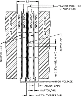
The read-out structure is based on the principle of an electrostatic transformer [8] (EST, see Fig. 2).

For each gap it consists of a central board, which contains the read-out electrode pads (PAD board), and two boards that are part of the ESTstructure (ESTboards). Each ESTboard is made of a layer of insulator (polyimide) sandwiched between two high resistive layers (HRL) that are connected to ground or high voltage (HV). The polyimide-based HRL material has a typical resistivity of 0.5 MO/

&. The PAD board is made of a copper read-out electrode sandwiched between two insulators and covered on both outside faces with a HRL, like the ESTboard. Thus in total a four subgap structure with one PAD and two ESTboards completes the electrostatic transformer structure. This yields in total 96 subgaps for HEC1 and 64 subgaps for HEC2. The high resistivity of the HRL yields a natural protection for the preamplifiers from potentially dangerous sparks in the argon gaps.

In addition it provides a simple distribution of the HV or ground across the area of the full board.

The space between the electrodes is maintained using honeycomb mats. The EST structure allows for a smaller gap design without increasing the overall capacitance. It decreases the required HV for a given electric field and shortens the drift time.

The low capacitance enables a fast signal rise and keeps the electronic noise low.

In order to limit the capacitance seen by a single preamplifier, only two gaps are ganged together at the pad level. A stripline connector of 50 O impedance running across the longitudinal section and coaxial cables running in between the sections carry the signal to the preamplifier boards located at the wheel periphery (see Fig. 1). These signals are amplified and summed employing the concept of ‘‘active pads’’: the signals from two consecutive pads are fed into separate preamplifiers (based on highly integrated GaAs electronics, see below).

The output signals from typically four preampli- fiers are summed together within the same preamplifier chip. A buffer stage drives the output signal up to the cold-to-warm feedthroughs. The use of cryogenic GaAs preamplifiers and summing amplifiers provides the optimum signal-to-noise ratio for the HEC. The total number of read-out channels for a single f-wedge consisting of a HEC1 and a HEC2 module is 88.

Modules are stacked at four institutes, from sub-components manufactured in industry and institutes. Manufactured modules are shipped to CERN. Careful Quality Control (QC) is required to assure a uniform conformance to design.

Central to this QC are mechanical and electrical tests upon receipt of a module at CERN, followed by a cold test or a particle beam test. An eighth of all modules are beam tested. All QC data are stored in a database which is available to all institutes involved. All important measurements, for example the total module thickness, are stored in this database. Fig. 3 shows a histogram of the module thickness acheived today in the 20 HEC1 and 13 HEC2 modules produced.

Copper plates are machined in industry and several institutes. The front module plates are manufactured from quarter hard cold rolled copper to provide sufficient strength, while the

Fig. 2. Schematic of the arrangement of the read-out structure in the 8.5 mm inter-plate gap.

rear module plates which are twice as thick and therefore about eight times stiffer are manufac- tured from hot rolled copper. Each batch from the rolling mill had a sample produced to allow for the copper density and strength to be checked. Every production facility had its machining and cleaning method qualified by producing a sample which was carefully checked for argon poisoning. Care had to be taken with the cold rolled copper to obtain the flatness tolerance of 0.5 mm because surface machining relieved stresses that could cause significant bowing. The 0.25 mm flatness tolerance on the rear plates was more easily obtained. The plate thickness tolerance is 7 0.05 ( 7 0.10) mm for the front (rear) plates. This tolerance can, during module stacking, cause an excessive buildup in the height of the module. This is corrected for during stacking by using slightly larger or smaller 8.5 mm gap defining annular spacers between the absorber plates to correct for any tolerance buildup.

Both PAD and ESTboards are manufactured in the institutes. These electrodes are manufactured from four main sub-components: 75 mm sheet polyimide, 25 mm sheet polyimide loaded with carbon with a typical resistivity of 0.5 MO/&, sheet glue, and copper clad polyimide etched with the electrode read-out structure. The electrodes are pie-shaped and are about 1.6 m long and 0.4 m wide at the wide end. In view of these dimensions care has to be taken when cutting polyimide materials due to the variation in dimension with humidity. Cutting, which is accomplished with a steel rule die (prefabricated high precision cutting

form), is undertaken only when the relative humidity is in the (45 7 10)% range. Manufacture of the electrodes is made following standard industry practices using a high-pressure press and an oven. Two electrical connections are made to every high resistive layer to provide connection redundancy, and to provide a more direct path for the significant currents that will be produced in the high eta region of the detector during high luminosity operation of the LHC. Alignment of materials in the electrodes is achieved at the 0.3 mm level. The electrodes are spaced by 1.85 mm insulating honeycomb mats. These mats are cut using a steel rule die. Every mat has its thickness measured, and every 20th mat is weighed.

In this way the signal reduction due to replacement of the liquid argon by honeycomb is established.

Boards containing glue from every batch of glue are tested in a high radiation environment, equivalent to 10 years of LHC operation. Sub- sequent to this irradiation the argon poisoning and peel strength is checked [9]. No significant dete- rioration was detected. In this way every batch of glue is qualified for use in the ATLAS experiment.

Every module is tested at the production site for 2 weeks at high voltage (2 kV). This procedure tests for any residual solvent bubbles that might be in the 75 mm sheet polyimide. The modules are then wrapped and shipped to CERN. Upon receipt at CERN modules undergo detailed electrical and mechanical QC tests, and then are cold tested. Modules are accepted from the cold test if they have one or no short. The shorted subgap, if present, is disconnected reducing the signal of the affected tower by 1/32nd or 1/64th depending on the location. The module is then stored for subsequent assembly into wheels.

2.3. Cold front-end electronics

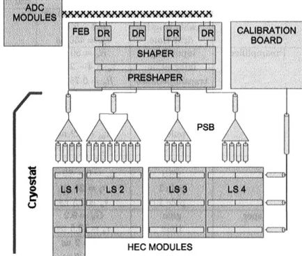
The read-out electronics as well as the calibra- tion electronics used in the beam test setup are very similar to the electronics to be used in the final ATLAS scheme. The read-out chain is schematically shown in Fig. 4.

The ionization signal from the liquid argon gap (or the calibration pulse) propagates via coaxial cables to the preamplifiers, where the signals from

Fig. 3. Histogram of the module height acheived to date in the 20 HEC1 and 13 HEC2 modules produced.

successive gaps are summed to one output channel. This output signal is then carried to the front-end board outside the cryostat.

A detailed description of the HEC front-end electronics can be found in two forth-coming papers [10,11]. Here we summarize the main characteristics which are important for the analysis of the beam test data (see Table 1). The detector capacitance C

affects the signal rise time, amplitude and signal-to-noise ratio. For different pads C

varies from 20 to 400 pF giving a wide distribution for the rise time and noise. The ionization current depends on the electrical field in the LAr gap. The values in Table 1 correspond to the nominal value of 1800 V for the high voltage.

The preamplifier ASIC is made by the GaAs TriQuint QED-A process. This technology has been chosen because it offers excellent high-fre- quency performance, low noise, stable operation at cryogenic temperatures and radiation hardness.

One chip contains eight identical preamplifiers and two drivers, giving the possibility to sum signals according to the physics requirements. The

Fig. 4. Schematic of the HEC beam test electronics, showing the longitudinal segments (LS), the preamplifying and summing boards (PSB), the front-end board (FEB), the FEB drivers (DR), the calibration board and the analog-to-digital converter (ADC) modules.

Table 1

The main electronic parameters of the detector and of the front- end electronics as well as the transfer functions used

Chain component

Parameters Values Transfer function Detector Capacitance CD=20–400 pF F

Cable length 0.2–2 m F Drift time tdr=450 ns F Preamplifier Input imp. Ra=50O

Integration ta=4–23 ns Rp

ð1þst_aÞð1þst_daÞ Transimpe-

dance

Rp=0.75 kO Driver tda=4 ns

Signal cable Attenuation as=0.965 asð1þstzsÞ ð1þstosÞð1þstpsÞ Zero tzs=24.5 ns

Pole 1 tos=1.2 ns Pole 1 tps=28.5 ns Preshaper Gain Gp=6.5

Zero t_pz=0–20 ns

Pole 1 t_i=29 ns G_pð1þst_pzÞ ð1þstiÞð1þstoÞ Pole 1 t_o=2.5 ns

Shaper Gain G_s=9.2

Time t_s=13.5 ns 3:69G_sst_s ð1þstsÞ³

Driver and Pole t_df=2 ns 1

ð1þst_dfÞð1þst_acÞ ADC cable Pole tac=7 ns

preamplifiers are placed on the outer radius of the calorimeter wheel inside the cryostat. Five pre- amplifying and summing boards (PSB) process signals from one HEC f-wedge (made of one HEC1 and one HEC2 module). They have 67 chips with 88 output channels in total. All signal and calibration cables are high-quality radiation resistant (made of PEEK) 50 O coaxial cables. The cable length from the pad to the preamplifier input is B 0.2 m for the outer region and B 2 m for the innermost part. The total length of the calibration cables in the beam test setup is 11.8 m (corre- sponding to 12.2 m in the final ATLAS detector) and the length of the signal cables is 8.3 m (corresponding to 8.7 m in the final ATLAS detector). Because of the substantial length of cables all effects due to signal attenuation and shape distortion have to be taken into account in the calibration procedure. The preamplifier and cable characteristics have been studied at room temperature and at liquid nitrogen temperatures.

Their transfer function has been parameterized in the frequency domain by two poles and by one zero and two poles. Typical values of the parameters are given in Table 1.

3. Particle beam tests

3.1. General beam test setup

The concept and the technology used for the construction of the hadronic end-cap calorimeter

have been verified in beam tests in the years 97–99 using either prototype modules or pre-production modules. The series ATLAS HEC modules are tested either in technical cold tests or in dedicated beam tests. These tests are part of the general quality control procedures to guarantee their successful operation in the ATLAS detector. The first two beam tests with series ATLAS HEC modules have been carried out in 2000. In each beam test three f-wedges (each made of one HEC1 and one HEC2 module) of the HEC have been tested. Simulation studies show that this setup yields a total leakage of incident pion energy below B 3.5% in the energy regime accessible. This rather low level of energy leakage allows a precise determination of the calorimeter performance parameters.

The beam tests have been carried out with a separated beam (H6) of the CERN SPS. It is a secondary or tertiary particle beam that provides hadrons, electrons or muons in the energy range 6pEp200 GeV: The beam intensity varies strongly with energy and particle type. Given the maximum trigger rate of 400 per burst that could be achieved, the particle intensity has been kept typically below 2000 particles per burst. The general setup is shown in Fig. 5. Using either three HEC1 or three HEC2 modules, a partial fraction of the HEM or HEC2 wheel, respectively, is assembled using the final wheel assembly techni- que. These HEC1 and HEC2 partial wheels are placed together in the beam test cryostat forming three full f-wedges of the HEC calorimeter. The

Fig. 5. The setup used for data taking in the beam tests. The trigger is defined by the scintillation counters B1, F1 and F2 and the scintillation counter walls VM, M1 and M2.

segmentation of the HEC is pseudopointing in Z and pointing in f in the ATLAS detector. In the beamtest the impact angle is constant, i.e. 90 1 with respect to the front plane, yielding for the energy reconstruction of particles a somewhat larger number of channels than in ATLAS. Fig. 6 shows a view of the two partial HEC wheels in the cryostat during the installation.

The cryostat with an inner diameter of 2.50 m and a fill height of LAr of 2.20 m can be moved horizontally by 7 30 cm. The beamline bending magnet closest to the experimental zone allows to deflect the beam vertically by 7 25 cm at the front face of the cryostat. Thus a scanning area of typically 60 50 cm

is available for horizontal and vertical scans. A beam window with reduced wall thickness (5.5 mm stainless steel in total and a diameter of 60 cm) of the cryostat minimizes the

dead material for particles prior to hitting the calorimeter within this area. In addition, a LAr excluder in front of the modules is installed for the same reason.

Fig. 5 shows the location of the trigger and veto counters. The beam trigger is derived from the signals of a differential Cherenkov counter for particle identification up to 80 GeV, of one up- stream scintillation counter (Bl), of three scintilla- tor walls (VM, M1, M2), and of two scintillation counters for fast timing (Fl, F2 with s=70 ps).

Impact position and angle of a beam particle have been determined using four multiwire proportional chambers (MWPC) with two planes (vertical and horizontal) per chamber. The wire spacing is 1 mm

(MWPC2, MWPC3, MWPC4) and 2 mm

(MWPC5), respectively. Veto counters (VM) are used to reject particles from the beam halo. To

Fig. 6. View of the setup of the HEC1 and HEC2 partial wheels in the cryostat. Each partial wheel is built out of three modules, the final calorimeter will have 32 modules per wheel.

also veto photons with high efficiency, an addi- tional lead layer has been added in front of the veto wall. Downstream of the cryostat an iron absorber with scintillation counter walls in front (M1) and behind (M2) is used for triggering or tagging muons.

3.2. Calorimeter operation

The cryogenic system has been operated from the common ATLAS beam test cryogenic system [12].

As described above, each LAr gap contains an electrostatic transformer structure (EST), which effectively divides the gap into four subgaps. The HV for these four subgaps is supplied by individual HV lines, which feed each longitudinal read-out segment separately. Typically not more than one HV line out of 48 had to be disconnected because of a HV problem in one subgap. With a total number of 480 subgaps this amounts to a subgap failure rate of 0.2%. It has been shown that the energy resolution is nevertheless recover- ableFexcept for an increased noise contribu- tion F by using simple multiplicative depth correction factors to offset the reduction of the signal in read-out segments affected. Because the distribution of HV lines is matched to the individual read-out segments the individual shower fluctuations are measured correctly, thus enabling a recovery of the energy resolution in case of minor HV problems.

Runs (typically 30,000 triggers) with random triggers only have been taken regularly to analyze the electronics performance with respect to elec- tronic noise and pedestal stability. In addition, random triggers have been taken in parallel with real particle triggers (typically at the level of 5%) to enable a continuous monitoring of these quantities and to study possible differences be- tween ‘‘in burst’’ and ‘‘out of burst’’ random triggers.

Data have been collected in two run periods, with typically 1000 runs per run period and about 20,000 triggers per run. The data quality has been monitored during data taking by running the online version of the offline reconstruction task [13]. All relevant quantities such as signal response

in the calorimeter, its spatial distribution and time evolution, the electronics performance, the MWPC response and efficiency as well as the trigger quantities have been continuously con- trolled during data taking.

3.3. Read-out electronics and DAQ 3.3.1. Read-out electronics

As shown in Fig. 4 the output signal of the cold summing amplifiers is carried to the front-end board (FEB) outside the cryostat where the analog signal shaping is performed. The crate with the FEB’s is installed directly on the cryostat feed- through, extending thus the Faraday cage of the cryostat. The rise time compensation is performed in the preshapers and the final pulse shape is formed by the shapers. The signal waveform is digitized by ADC modules and the data are transferred via the VME bus to the data acquisi- tion system.

Three FEB’s with 128 channels per board pro- cess the signals from up to four HEC f-wedges.

The FEB used in the beam test is a prototype board of the final ATLAS board (only the analog part is present). The preshapers equalize the signal rise time by the pole-zero cancellation method.

Each individual channel is adjusted to the expected value of the detector capacitance, giving 14 different time constants in total. An additional integration is introduced in order to reach a peaking time of 50 ns at the output of the chain.

The signal is also inverted and amplified in the

preshaper in order to adapt to the working range

of the shaper. The amplification for the HEC2

modules is a factor of two higher to compensate

for the smaller sampling ratios in these calorimeter

modules. One preshaper hybrid contains four

channels corresponding to the four longitudinal

HEC channels with the same Z and f location in

ATLAS. The final signal shape is formed by a

RC

CR monolithic shaper with a time constant

of about 14 ns and a gain of 10. One FEB is

equipped with 32 four-channel chips. The shaper

chips are of the final ATLAS version, the detailed

information can be found in Ref. [14]. The

unipolar signals from the shaper output are

converted to differential signals by the FEB

drivers. This component is specific to the beam test setup and will not be present in the final ATLAS scheme. The signals from the FEB are routed to the ADC modules via 3 m long twisted pair cables.

All parameters of the components of the electronic chain have been determined from measurements either in the laboratory or in the real beam test setup. To obtain a detailed description of the signal shape, the integration in the driver and the distortion in the cable are also taken into account (see the last row of Table 1).

The numbers presented in Table 1 are averaged values. The overall transfer function of the signal chain is the product of all functions in the last column. This function consists of two zeros and nine poles, and it is used to describe the calibration and ionization signals.

An event trigger stops the digitization and outputs of the ADC chip are disabled. The signals from the FEB boards are digitized by twelve 32- channel ADC modules, installed close to the cryostat. The modules are VME-9U boards. Each motherboard contains eight plug-in units with four digitizing channels. The signal is sampled every 25 ns using a 12-bit ADC chip (Burr-Brown Model ADS800) and stored into a 256-cells circular- RAM with 10 ns access time. As the next step the CPU reads the RAM content in a block-transfer mode through the VME Bus. The ADC input signal range of 7 2 V yields a conversion factor of 1 mV per ADC count. Each line of the differential input signal is terminated by a 50 O resistor, connected to an adjustable voltage level. This level is used to shift the pedestal level to B800 ADC counts in order to get the negative part of the signal digitized as well. The ADC has an integral nonlinearity of 72 LSB and a differential linearity error of 70.6 LSB.

3.3.2. Data acquisition system

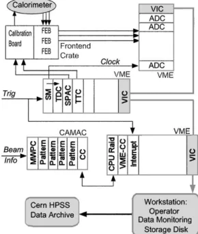
The data acquisition is based on a multi-crate VME system, connected by a VME interconnect bus VIC [15]. The block diagram is shown in Fig. 7. The ADC modules are read via their VME bus interface by a single RISC CPU module (MIPS 3000 based CES RAID, running the real time system CDC EP/LX [16]). In addition, the relative time of the pretrigger to the 40 MHz ADC

clock is read from a TDC module. The beam information, i.e. the MWPC electronics (PICOS-II system) and pattern units for the scintillation counters, is read via a CAMAC system. During one SPS burst the data are buffered in the RISC CPU, then copied to an HP workstation (type HP 9000/748) and recorded on disk. Given an event size of B 13 kbyte, resulting from the read-out of 16 time samples per ADC channel, the VME access to the ADC data via the VIC bus and the CAMAC read-out limit the data rate to approxi- mately 300 events per SPS burst (B2.5 s). The workstation, in addition to its role as a data recorder, serves as online data monitor providing histograms and performance checks. The data are sent to CERN’s HPSS storage library asynchro- nously to the data acquisition through a network file copy.

3.4. Calibration and signal processing

The main purpose of the calibration of the electronic chain is to equalize the gains of all channels and to correct any nonlinearity of the response. Calibration errors normally result in an

Fig. 7. Block diagram of the data acquisition system.

increase of the constant term in the energy resolution. The system has to keep track of the timing stability and, if necessary, provide correc- tions. Another goal of the calibration is to measure the signal shape and the noise autocorrelation function. This information is used to produce weights for the digital filtering algorithm (see below). Finally the calibration system is used to determine the inter-channel cross-talk, which is important for an accurate energy reconstruction.

The calibration board contains 128 pulse gen- erators and is installed in the front-end crate. This board is a pre-series module of the final ATLAS board [17]. The voltage pulse from one generator is guided through coaxial cables to a strip line board located close to the detector pads. Each generator signal is split into three on the calibration distribution board (placed at the back plane of each HEC module) in order to reduce the number of cables and feedthrough connectors. Each of these three signals pulses up to 16 preamplifiers via high precision calibration resistors located on the strip line board. In total 16 generators are used for one HEC f-wedge. The strip line board is mounted in parallel to the beam direction in notches in the copper plates, close enough to the pads, so that the delays of calibration pulses to different pads approximately mimic the particle signal timing. The calibration procedure is de- scribed in detail in Ref. [18]. It consists typically of four different steps: (i) measurement of gain and nonlinearity by pulsing all the channels with different pulse levels, (ii) measurement of signal shape by performing either delay scans (25 ns range with 1 ns steps) synchronous with the trigger, or, in asynchronous mode, determining the time by the TDC module, (iii) measurement of cross-talk by simultaneously pulsing one or a few generators and reading all neighboring channels, and (iv) measurements of noise with all generators switched off. A minor change was made to the standard LAr calibration board, in order for it to be compatible with the overall beam test setup: the internal resynchronization of the pulse with the clock has been switched off. Instead a VME-based module, called a Service Module (SM), has been used for the generation of the 40 MHz clock and of the timing of the calibration pulse command. The

SM also produces the start and stop signals for the TDC module, which measures the time delay between the trigger and the clock pulse. The communication with the calibration board is done via the VME based SPAC and TTC modules [19].

The steering software is a modular system, which practically allows any type of measurements either in the time of setting up and debugging the electronics or during standard calibration runs.

The measured data are transferred via direct memory access (DMA) in VME from the ADC boards to the RAID computer and sent to the HP computer for storing. For this operation the CALTCP protocol is used, an OO protocol, which is based on TCP/IP and is highly optimized for speed [20]. The additional visualization tools are based to a large extent on a ROOTlibrary [21].

For the amplitude reconstruction, the weighted sum of five signal samples (or four samples and pedestal) will be implemented in ATLAS [22,23].

The same approach has been chosen for the beam test data analysis. The energy deposited in the read-out cell is calculated as

E

¼ X

n¼1

W

U

ð1Þ

where W

are predefined weights and U

are the

measured signal samples. The weights are deter-

mined by minimizing the noise-to-signal ratio and

are calculated from the ionization signal shape and

noise autocorrelation coefficients [22]. One of the

important steps in the calibration analysis is the

prediction of the particle waveform on the basis of

the calibration shape measurements. This predic-

tion is obtained by fitting the calibration signal

with a model function and extracting two time

constants: the preshaper integration time t

and

the shaper time t

: The particle signal shape is then

calculated by a convolution of the electronic chain

response with the triangular ionization current

from a real signal. The model function for the

calibration signal is obtained from the parameter-

ization of all components of the calibration chain,

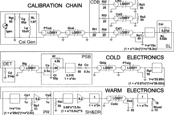
shown (together with the full signal chain) in

Fig. 8. The parameterization is similar to the one

used for the signal chain description. It is derived

from oscilloscope measurements in the laboratory

and in the beam setup. The functions and parameters are given in Table 2.

In order to minimize the CPU time for the analysis, an analytical expression for the signal shape has been derived. The full function for the calibration signal in the frequency domain consists of 12 poles and 4 zeros, which would give an extremely complicated expression in the time

domain. For the analysis of the data this function has been simplified by removing a few minor parts.

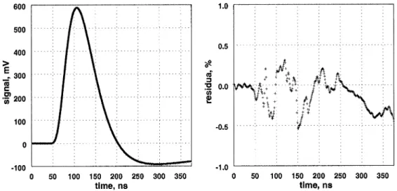
The quality of the fit to the calibration signal and the ionization signal prediction are illustrated in Fig. 9. Typical residuals (shown in the lower figures) are 70.5% for the calibration pulse and 71.5% for the ionization signal. The fit is performed only for the positive part of the signal wave since only this region is used for the energy determination.

The transformation from ADC counts to current is accomplished using a third-order poly- nomial function. The related coefficients have been determined from the fit of the calibration ampli- tude ramp. The amplitude of the calibration pulse is determined by applying weights similar to the ones used in Eq. (1). In this case the weights are derived from the calibration pulse shape and differ from the weights applied to the real ionization signal. The typical nonlinearity for the energy

Fig. 8. Schematics of the HEC electronic chain, showing the calibration generator board, the preshaper (PR), the shaper and FEB driver (SH&DR) located in the warm and the calibration distribution board (CDB), the strip line (SL), the detector gap (DET) and the preamplifier and summing board (PSB) located in the cold LAr.

Table 2

Parameters of the calibration signal and model functions Chain

component

Parameters Values Model function Generator Decay time td=350 ns aþst_d sð1þstdÞ Step fraction a=0.07

Cables Attenuation a_c=0.905 Zero t_zc=18 ns

Pole 1 t_oc=1.2 ns a_cð1þst_zcÞ ð1þstocÞð1þstpcÞ Pole 2 t_pc=21 ns

range accessible in the beam exposures is B1%.

But the calibration generators have some parasitic effects at low amplitudes [17], which makes a precise calibration in the region of the muon signal rather difficult.

3.5. Liquid argon purity monitoring

The purity monitoring system utilizes two different radioactive sources which provide the means to ionize the liquid argon. The liberated charge is collected and the mean measured signal is used to determine the O

concentration [24].

The first system consists of an

Am source which provides 5 MeV a particles. The range of a particles in the LAr is only approximately 100 mm, hence the ionization density is very high. The

deposited charge is collected over a gap of 2 mm at an electric field strength of 12.5 kV/cm. The colle- cted charge for pure argon is about 5 fC. For an impurity caused by oxygen, the signal decreases nearly linearly with the oxygen concentration.

The second system employs a

Bi source. It provides mono energetic 1 MeV electrons from an electron conversion process. The electrons have a mean range of 3 mm in LAr. The 6 mm wide LAr gap is separated by a Frisch-grid [24] into two compartments of 5 and 1 mm each, with an electrical field strength of 5 and 25 kV/cm, respectively. The electron deposits its energy in the 5 mm gap. The liberated charge drifts through the grid into the second compartment, which is attached to a charge sensitive amplifier. In this way the signal does not depend strongly on the track

Fig. 9. The calibration signal (left) and the prediction for the ionization signal (right) together with the residuals with respect to the fit (lower figures).

length or on the emission angle of the electron, resulting in an increased sensitivity to impurities.

A quadratic dependence on the O

concentration is expected.

Both cells are simultaneously read out by a single charge sensitive amplifier

which is located next to the cells in the LAr. The signals from the two sources are distinguished by their different sign (positive for the

Am cell and negative for the

Bi cell). From the ratio of the measured signals of the two cells the O

contamination is estimated. In order to determine the absolute O

concentration the signal ratio has been measured in a test cryostat as function of a known O

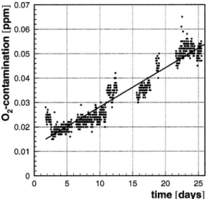
contamination. The systematic uncertainty of this measurement is about 30%. The measured con- tamination over a period of 25 days during the beam test is shown in Fig. 10. An increase of the oxygen contamination of approximately 1.6 ppb/

day has been observed, starting from about 12 ppb at the beginning of the run period up to about 52 ppb at the end of the run period. This rather small increase is attributed to intrinsic leaks in the

cryogenic system. The visible variations of the measured contamination are due to a temperature dependence of the high-voltage system for which no correction has been applied.

3.6. Liquid argon temperature monitoring

The temperature of the LAr as well as that of the copper absorber plates have been monitored constantly during the cryogenic operation. Plati- num PT-100 temperature sensors have been chosen because of the proven long-term stability and low sensitivity to magnetic fields. In addition, radiation tests with neutrons and photons have shown that the sensors withstand high radiation levels and still offer a high sensitivity in the temperature range of interest, i.e. 70–90 K. The small geometrical size as well as the low price are also advantageous. A special calibration procedure of the sensors has been carried out to achieve a precision of typically 6–8 mK during operation.

There are two separate sets of temperature sensors: one set monitors the temperature of the argon and a second set monitors the temperature of the modules.

The set that monitors the argon is made up of eight regular PT-100 probes as well as of two high precision probes. The regular probes are mounted in copper blocks and positioned at different heights inside a tube of 1600 mm length running vertically inside the cryostat [25]. Each high precision probe is placed next to a regular probe and is used as a reference system. All these probes allow for the control of the process of warming up and cooling down as well as the monitoring of the temperature gradient in the liquid argon.

Six additional probes have been installed at the rear plates of individual modules, as foreseen in the final HEC wheel assembly. These probes monitor the module temperature in particular during the cool down and warm up operations.

A precise resistive direct current bridge is used for the measurement. Two different systems have been used for the signal readout: a 16-bit digital- to-analog converter (DAC) in combination with a microprocessor (DUBNA-4 system) and a local monitoring box (LMB) developed at CERN as

Fig. 10. O2 contamination estimated from the signal ratio of the²⁴¹Am cell and ²⁰⁷Bi cell. An increase of 1.6 ppb/day has been observed during the run period.

12The cold preamplifiers for the purity monitoring system were developed and kindly provided by V. Radeka (Brookha- ven National Laboratory, NY, USA).

part of the general detector control system (DCS) used in LHC experiments. Both measurement systems gave fully consistent results.

Fig. 11 shows the time dependence of the LAr temperature as measured by the various sensors positioned either at different height in a tube inside the cryostat (S) or at the rear plates of individual modules (P) over a time period of 12 h. The temperature stability of the LAr over a long period of time was typically in the range of 20–30 mK, except for short periods corresponding to the refilling of the phase separator dewar. For example Fig. 12 shows the distribution of the temperature measurements as obtained from a single probe (S1) during a 12 h period. In this case the stability reached is about 2.5 mK rms.

4. Data analysis and simulation

4.1. Data analysis and signal processing

About 1000 runs with electron, pion or muon data have been taken in each run period. Energy scans in the range 6 o E o 200 GeV have been performed for electrons and pions at 15 different impact points covering the area accessible through the beam window of the cryostat. Within this region the amount of dead material in front of the calorimeter setup is minimal. Fig. 13 shows the beam impact points (labeled as A–O) on the front face of the three HEC f-wedges. These impact points have been selected using simulations of electron data. Their distance to the tie rods (open circles) is large enough to keep signal losses at an acceptable level. In addition, horizontal and vertical scans have been performed for all particle types and at various energies.

For the nominal high voltage (1800 V) the electron drift time for the HEC LAr gap is 450 ns, so the full signal covers 21 or 22 time samples each separated by 25 ns. For each event trigger, 16 time samples have been read out. In specific runs, e.g. scans in the area near the edge of modules, data taken at lower HV settings or studies for the analysis of the full signal shape, an even larger number of time samples (up to 96) has been used. The signal amplitude has been recon- structed using the optimal filtering technique [22]

and the calibration constants. Out of the 16 time samples, five (from the 7th to the 11th) have been used for this reconstruction. The precision of the signal amplitude reconstruction is typically 0.5%.

An important aspect is the quality of the signal waveform description. For a typical read-out channel, Fig. 14 shows the reconstructed normal- ized waveform for electron data. For each event the signal in each time sample is normalized using the reconstructed amplitude. The maximum is expected to be at 1.0 for a perfect signal wave- form reconstruction. The observed deviation is about 7 0.5% reflecting the accuracy of the procedure applied. This precision depends criti- cally on the parameterization of the particle signal as predicted from calibration data. The first five time samples preceding the event pulse

Fig. 11. Time dependence of the liquid argon temperature as measured by five sensors positioned either in a tube at different height (S) or at the rear plates of individual modules (P).

Fig. 12. Distribution of the liquid argon temperature measure- ments as obtained from a single probe (S1) during a 12 h operation period.

are used to define the pedestal value and the noise (again using the optimal filtering technique) of each individual read-out channel. The noise suppression factor from optimal filtering is typi- cally s

=s

E0:620:7; where s

refers to the spread of the electronic noise seen in an individual time sample. The ADC clock is not synchronized with the particle trigger, therefore the start of the signal is randomly distributed within a range of 25 ns with respect to the clock signal. The timing information is supplied by the TDC module and used to predict the signal position within the ADC window. The dependence of the optimal filtering weights on the TDC data is obtained from the analysis of calibration data. The time dependence of each weight is parameterized by a fourth-order polynomial. The parameterized

Fig. 13. The beam impact points (open squares) on the front face of the calorimeter setup with threef-wedges. Data taken at these points have been used for the energy scans. The open circles locate the tie rods. The dashed circle represents the area accessible through the cryostat window, while the dashed rectangle represents the area accessible through beam bending (vertical) and cryostat motion (horizontal).

Fig. 14. Reconstructed normalized signal waveform for elec- trons of different energies.

functions are used to calculate the weights for each event.

Due to thicker copper absorber plates, the HEC2 wheel has a sampling ratio which is smaller by a factor of two with respect to the HEC1 wheel.

Therefore the visible energy E

for HEC2 has been multiplied by a factor of two prior to extracting any calibration constant. For the long- itudinal segment with one HV line disconnected a geometrical correction factor of 4/3 has also been applied.

To reconstruct the energy, clusters of cells have been defined in each longitudinal segment. The cluster size has been kept fixed for each impact point so that the noise contribution can be better studied and controlled. Read-out channels near each impact point were included if they had an average signal of more than 200 nA for electrons at 175 GeV or 15 nA for pions at 180 GeV. This selection yields a typical cluster size of 6 read-out channels for electrons and about 50–60 read-out channels for pions. Rather large cluster sizes have been chosen in order to keep losses due to energy leakage small. Simulation studies give an estimated energy leakage of B 0.4% for electrons and B 5%

for pions. For pions this is dominated by energy leakage outside the three HEC f-wedges, which is typically at the level of B 3.5%. To estimate the electronic noise contribution, the noise from the cluster channels has been summed. Thus any correlation between different channels or any coherent part in the noise is automatically taken into account. This holds since the noise in the calibration data, which are used to extract the optimal filtering weights, is similar to the noise in the particle data. Given these cluster sizes, the equivalent noise amounts to B0.6 GeV for elec- trons and B6 GeV for pions.

All data have been processed using the standard HEC offline reconstruction program [13], which comprises pedestal and signal amplitude recon- struction as well as trigger handling, cluster reconstruction and slow control data monitoring.

4.2. Monte Carlo simulation

The evaluation of the HEC performance re- quires the comparison of experimental data,

obtained at beam tests, with detailed Monte Carlo simulations. To fulfil this task a special software package has been prepared [26]. It allows for the simulation of the response of the HEC modules to various particle beams of different energies, avail- able at CERN beam tests. This package uses the standard ATLAS software [27] (DICE 3, ATL- SIM) with GEANT3.21 [28] for the detector response simulation.

The geometry of the beam test setup is described in full detail. For example, the HEC module description includes not only copper plates and gaps of liquid argon, but also polyimide electrodes, copper pads and tie-rods. All H6 beam elements, such as the cryostat, multiwire proportional chambers and scintillating counters, extended over a distance of 30 m, are included as well. Three different codes for the hadronic shower develop- ment, GFLUKA, GCALOR and GHEISHA, are available for simulations,

Prior to the analysis of simulated events, hardware conditions (e.g. reduced signal in in- dividual gaps due to disconnected HV lines) have been taken into account. For the electron and pion beam test data the actual noise has been sub- tracted. For muon simulation the actual electronic noise has been added to the signal using beam test events. For each read-out channel and each individual event the noise has been added to the simulation with a scale factor k ¼ a

=a

; transforming the noise from the nA scale to the GeV scale of visible energy. Here a

is a dimen- sionless ratio E

= / E

S ¼ 23:3070:01;

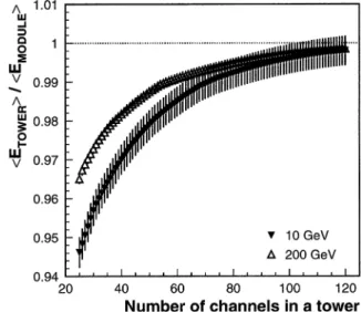
found using electron MC samples. The difference in sampling ratios between the HEC1 and HEC2 wheel has been included. The leakage of energy of electromagnetic showers out of a selected cluster (see Fig. 15) has been taken into account in the determination of the scale factor k: All the procedures and program chains, which were used to analyse Monte Carlo events (after hardware corrections described above), are exactly the same as those used for the beam test data.

The layout of the HEC beam test setup with

only three f-wedges and the absence of an

electromagnetic calorimeter in front, causes a

problem with respect to the longitudinal and

lateral leakage of energy for hadronic showers.

To estimate the influence of the energy leakage on the performance of the calorimeter, ‘‘virtual’’

leakage detectors are implemented. In these leakage detectors the kinetic energy is summed up for all particles leaving the HEC modules through lateral and back sides.

Fig. 16 shows the energy dependence of the total energy leakage as well as lateral and longitudinal

ones as expected from Monte Carlo simulations for pions at a central impact point. For all energies the fraction of energy lost is typically at the level of 3–3.5%. At low pion energies the losses are dominated by the lateral leakage due to the limitation to three f-wedges. At high energies the longitudinal leakage starts to play a role as well.

The leakage of energy of hadronic showers out of the selected cluster (see Fig. 17) is usually smaller than the leakage outside the HEC modules.

5. Calibration results

5.1. High-voltage curve

The basic characteristics of the liquid argon calorimeter which determine the ionization signal waveform for beam particles are the initial ionization current and the electron drift time.

Both parameters depend on the electric field in the liquid argon gap. To determine these quantities, special measurements have been performed.

For these studies electrons with an energy of 148 GeV at two different impact points (J and K, see Fig. 13), i.e. two different HEC modules, have

Fig. 15. The relative amount of the energy in a cluster with respect to the total visible energy in HEC modules for electrons as a function of the number of read-out channels used in the cluster.

Fig. 16. The relative amount of the leakage energy with respect to the pion beam energy as a function of the beam energy.

Fig. 17. The relative amount of the energy in a cluster with respect to the total visible energy in all HEC modules for charged pions as a function of the number of readout channels used in the cluster.

been used. The HV has been varied in the range 200–1900 V. In order to read out the full signal shape, the ADC time window has been increased to 96 time slices for low HV values. The main part of the deposited energy for electromagnetic showers is in a single channel of the first long- itudinal segment. These signals have been used in the analysis.

The determination of the ionization signal parameters has been performed in three steps. In the first step the calibration signal has been used to determine the electronics chain transfer function (see Table 1). Three parameters, the gain and the time constants of the preshaper and of the shaper, have been obtained. All other chain parameters have been kept fixed at their nominal values.

Fig. 18 shows the measured calibration data and the result of the fit (solid line) for the read-out channel related to the impact point J. Also shown are the residuals from the fit: a precision of 70.5%

is achieved, this holds also for the second read-out channel related to the impact point K.

In a second step the analytical function for the ionization signal in the time domain has been derived. Finally this function has been applied to the measured signals to determine the initial ionization current and the electron drift time t

: The measured and predicted ionization signals at two HV settings for the read-out channel related to

the impact point J are shown in Fig. 19. The precision of the signal shape prediction is within 71% for both channels and for all HV settings.

The drift velocity and electric field have been calculated using the nominal value of the liquid argon subgap thickness of 1.97 mm. Fig. 20 shows the drift velocity determined for the impact point J (circles) and point K (squares). During these measurements the variation of the argon tempera- ture was in the range 89.45–89.65 K. The solid lines in Fig. 20 presents the calculated drift velocity for the median temperature of 89.55 K using the parameterization [29]. Our data seem to indicate a somewhat longer drift time, the differ- ence being typically 1–2%. The initial ionization current depends on the electric field due to two reasons: for an increase in the electric field, (i) the drift velocity increases, and (ii) the primary recombination decreases. The second effect can be described by the Thomas–Imel model [30] as follows:

Q

¼ Q

lnð1 þ C=EÞ

C=E ð2Þ

where Q

is the ionization charge released, Q

is the ionization charge in the case of an infinite electric field (no recombination), and C=0.84 kV/cm is a constant. The ionization current is calculated from the charge using the measured drift time. Fig. 21

Fig. 18. Calibration signal: measured data (points) and the result from the fit (solid line) for the read-out channel related to the impact point J (left figure) and the residuals from the fit (right figure).

shows the data as well as the fit of the data to the Thomas–Imel model as given by Eq. (2).

From the value of Q

and the ionization energy per electron–ion pair of 23.2 eV (see Ref. [31] and references therein) the energy deposited in the liquid argon gap can be calculated. The values of 5.53 GeV for the impact point J and 5.60 GeV for the impact point K have been obtained. The corresponding values obtained from simulation using GEANT3 are 5.53 and 5.58 GeV, respec- tively. The systematic error on this prediction is estimated to be +1% due to different energy cuts

in GEANT3 and 2% due to the passive volume of the honeycomb spacer mats which are not included in the simulation. The agreement with data is within errors.

5.2. Response to electrons

The deposited energy, as reconstructed from the cluster, is obtained in units of nA and has to be converted to the related particle energy. To do so, an average scale factor a

=2.9370.03 MeV/nA has been obtained for the data. This electromagnetic

Fig. 19. Ionization signal from electrons. Shown are the data for two different HV settings for the read-out channel related to the impact point J (left figures). Also shown are the predicted signals (solid line) and the related residuals (right figures).

Fig. 20. The dependence of the electron drift velocity on the electric field. Shown are the data for the read-out channels related to two different impact point (dots and squares). The solid line represents recently published data (see text for reference).

Fig. 21. The initial ionization current (points) and the fit to the Thomas–Imel model (solid lines) for the two impact points.

calibration constant has been applied to the electron data for all energies. Fig. 22 shows the energy distribution of electrons with an energy of 10, 20, 80 and 147.8 GeV at a particular impact point. The solid lines represent Gaussian fits to the distributions within a region of 72s around the mean value.

Fig. 23 shows the energy dependence of the energy resolution s=E for electrons at three different beam particle impact points. The electro- nic noise in the related electron cluster has been obtained as described above and it has been subtracted quadratically for each individual en- ergy and impact point. Thus any time or impact point dependence of the electronic noise has been taken into account, as well as the contribution due to coherent noise effects (see discussion above).

The energy dependence of the energy resolution has been parameterized by

sðEÞ

E ¼ a

ffiffiffiffi E p "b

with a being the sampling term and b the constant term. The lines show the result of the fit to these data points using the ansatz given above.

The results for the sampling term a and the constant term b obtained for the various beam particle impact points are shown in Fig. 24. The average values obtained are a=(21.4 7 0.2)%

GeV

and b ¼ ð0:3 7 0:2Þ%; to be compared with simulation expectation of a ¼ ð21:7 7 0:1Þ% GeV

and b ¼ ð0:070:2Þ%: The data as well as the expectation (solid line, the error indicated by the dashed lines) are shown. The agreement is rather good. An important aspect of the calorimeter performance is the spatial uniformity of the response. This aspect can be tested by comparing data from different beam impact points. Fig. 25 shows the relative variation of the electromagnetic calibration constant a

with the beam particle impact position. The data are in a band of typically 7 1%, leaving not much room for any channel intercalibration errors.

Finally the linearity of the signal response has been studied as well. Fig. 26 shows the relative variation of the inverse of the electromagnetic calibration constant a

with beam energy. The circles show the results for the data at four

Fig. 22. Energy distribution for electrons with an energy of 10, 20, 80 and 147.8 GeV.

Fig. 23. Energy dependence of the energy resolution for electrons at three different beam particle impact points.

different impact points and the stars the corre- sponding expectations from simulation. The re- sponse is linear within a band of 7 1%. The decrease of the response at very low energy is mainly due to the dead material (0:6X

) in front of the calorimeter.

5.3. Response to muons

The muon data are essential to obtain informa- tion on the calorimeter response in the region of low deposited energy. In addition, horizontal and vertical scans test the homogeneity of the calori- meter at full depth.

Muon data have been taken at energies of 120, 150 and 180 GeV in the two run periods. The MWPC data have been used to reconstruct the beam particle trajectories. The extrapolation of these trajectories has been used to define the readout channels where the muon signal is expected. The impact angle of particles is 90 1 at

Fig. 24. Energy resolution for electrons at different beam particle impact points: shown (circles) are the sampling terma (top) and constant termb(bottom) as obtained from a fit to the beam test data (see text). The horizontal lines and the numbers show the expectation from simulation.

Fig. 25. Spatial uniformity of the signal response of electrons:

shown is the variation of the electromagnetic calibration constantaem with the beam particle impact position relative to the averageaem:

Fig. 26. Linearity of the signal response of electrons at four different impact points: shown is the relative variation of the inverse of the electromagnetic calibration constant a_em with beam energy.

all impact positions. In consequence the read-out structure is, in contrast to the final situation in the ATLAS detector, non ‘‘pseudo-pointing’’ in Z:

Therefore the typical number of read-out channels used for the energy reconstruction is typically six instead of four as for the ATLAS setup. Conse- quently, the noise contribution to the muon signal is increased accordingly. Simulation studies show that the losses of the visible energy due to the reconstruction algorithm are at the level of about 1–2% only.

Fig. 27 shows the comparison of the total energy deposited with the noise contribution for 180 GeV muons. The distributions are plotted in units of the noise width s

, the ratio of the muon signal to the noise is B 5. Fig. 28 compares the response with expectations for muons of 120 GeV. For the simulation the GEANT3 code has been used. The distribution of the data, which is covering more than four orders of magnitude in signal height, is well described by the simulation.

Horizontal and vertical scans have been carried out at various impact points and at all energies.

Fig. 29 shows the result of the horizontal scan with muons of energy of 180 GeV across the total accessible region, i.e. almost all three f-wedges of the test beam setup. Shown is the reponse in each individual longitudinal segment. Clearly visible are the positions of the two cracks between the

modules. The data reflect also clearly the long- itudinal calorimeter structure: eight LAr gaps for the segments one, three and four and 16 LAr gaps for the segment two. The reduced signal in the first longitudinal segment, typically 12% with respect to the third segment, compares within errors with the expectation of 11%. This reduction of the signal is due to the reduced contribution of the g

Fig. 27. Response distribution for 180 GeV muons (dashed line) in units ofsnoise;and the noise distribution (solid line).

Fig. 28. Response distribution for 120 GeV muons, shown for beam test data (full circles) and simulation (open circles).

Fig. 29. Horizontal scan with muons of 180 GeV extending over almost the fullf-range accessible. Shown is the reponse in each individual longitudinal segment. Clearly visible are the positions of the two crack zones between neighboring modules.

radiation to the muon signal in the first long- itudinal segment. These distributions are shown in more detail in the Fig. 30 for the two crack regions between the neighboring f-wedges. The lines shown reflect Gaussian fits in the crack zones to guide the eye. The dip structure in segment three is somewhat broader, reflecting a larger crack size of HEC2 (segment three only) at this particular height due to additional notches in the copper plates for the signal lines.

Finally the electron-to-muon ratio has been extracted from the data. All results have been corrected for minor shifts due to noise contribu- tions. For the most probable muon signal we obtain 0.93 7 0.02 for muons of 150 GeV and 0.92 7 0.02 for muons of 180 GeV. These results have to be compared with the MC expectations of 0.9170.01 at 150 GeV and 0.9270.01 at 180 GeV.

Using a truncated mean rather than the most probable value the corresponding numbers for the data are 0.9970.02 at 150 and 180 GeV. Here the corresponding MC prediction is 0.9570.02 at 150 GeV and 0.9670.02 at 180 GeV. The systema- tic error has been estimated using the maximum and minimum values obtained using different calibration runs or data at different impact points and varying the analysis cuts used. The electron- to-muon ratio can also be obtained using only the

reponse in HEC1 or the total response in HEC1 and HEC2. Again, the maximum and minimum values obtained have been used to estimate the systematic error. From these studies we estimate the systematic error to be 70.03. The agreement between the data and the simulation is within errors.

Finally the data have been used to extract the electron to MIP (minimum ionizing particle) ratio.

For this study the muon response at 150 GeV in HEC1 has been used. The fractions of the ionization and electromagnetic energy deposit of muons in the energy range considered have been obtained from MC studies. For the electron-to- MIP ratio a value of 0.99 7 0.02 has been obtained.

This result has to be compared with the MC prediction of 0.94. Taking the systematic error into account, the agreement is reasonable.

5.4. Response to pions 5.4.1. Energy reconstruction

The total energy has been reconstructed using one hadronic calibration constant. Since the HEC is a non-compensating calorimeter, i.e. the e=p ratio is energy dependent, this constant has been determined for each individual energy separately.

To reconstruct the total energy, the signals in all read-out channels of the related cluster have been summed. The factor a

; transforming the visible energy E

to the beam particle energy at a given nominal beam energy E

; is obtained from the ratio

a

ðE

Þ ¼ E

=E

: ð3Þ Fig. 31 shows for a given impact point the reconstructed pion signal at four different energies.

To determine the width s and the maximum position E

of the energy distribution, a Gaussian fit (solid line) has been applied to the data. The fits have an acceptable w

but the distributions are slightly asymmetric due to enhanced low-energy tails. Therefore the fit region has been limited to the interval E

7 2s to reduce the influence of these tails on the result. The Fig. 32 shows the energy dependence of the hadronic calibration constant a

at four different

Fig. 30. Horizontal scan with muons of 180 GeV. Shown is the signal in the two crack zones between neighboringf-wedges in each individual longitudinal segment.

impact points. It reflects directly the energy dependence of the e=p ratio of the HEC.

5.4.2. Energy resolution

Fig. 33 shows the energy dependence of the energy resolution s=E for three different impact points. The noise as measured in the correspond- ing cluster, has been subtracted quadratically at each energy point. The resulting energy depen- dence may be parameterized using

sðEÞ=E ¼ a ffiffiffiffi E

p " b: ð4Þ

where a represents the sampling term and b the constant term. The lines indicate the results of the fits. For the data the fit yields typically a ¼ ð70:671:5Þ% GeV

and b ¼ ð5:870:2Þ%: The data have been compared to the prediction from simulation, using GFLUKA, GCALOR and GHEISHA for the hadronic shower simulation.

In general GCALOR yields the best description of the data, but still being not quite optimal. Fig. 34

Fig. 31. The reconstructed pion response at four different energies for a given impact point, showing the reconstructed energy E₀ (GeV), the width s (GeV) and the corres- pondingw² per number of degrees of freedom (ndf) of the fit (see text).

Fig. 32. Energy dependence of the hadronic calibration con- stant at four different impact positions.

Fig. 33. The energy dependence of the pion energy resolution.

Shown are the data for three different impact points. The lines show the result of the individual fits (see text).