Fig. S1: Study Area: The ocean bottom seismometer (OBS) seismic survey near the Mid- Atlantic Ridge (MAR) in the equatorial Atlantic Ocean. The dashed red line refers to the MAR, and the triangles show the locations of the OBSs used for this study. OBS 55-59 (yellow
triangles) have been labelled, with the seismograms shown in Figs. 3 and S7-S10. The bold black line passing through OBSs shows the part of shot profile used, and the two pink bars indicate the part of the seismic images shown in Figs. 2, S3 and S4. The black line parallel shows the
distance from the MAR. The contour labelling 10 indicates the lithospheric age of 10 Ma. See the inset map for the location of the study area.
Fig. S2: Data for OBS 58 after pre-processing: Pg, PmP and Pn arrivals have been labelled in the pressure-component data. The data will be used for FWI after time-windowing for isolating Pg arrivals.
−5 0 −4 0 −3 0 −2 0 −1 0 Offset (km)0 1 0 2 0 3 0 4 0 5 0
2 4 6 8 1 0
Traveltime(s)
OBS 5 8
Pg
PmP
Pn
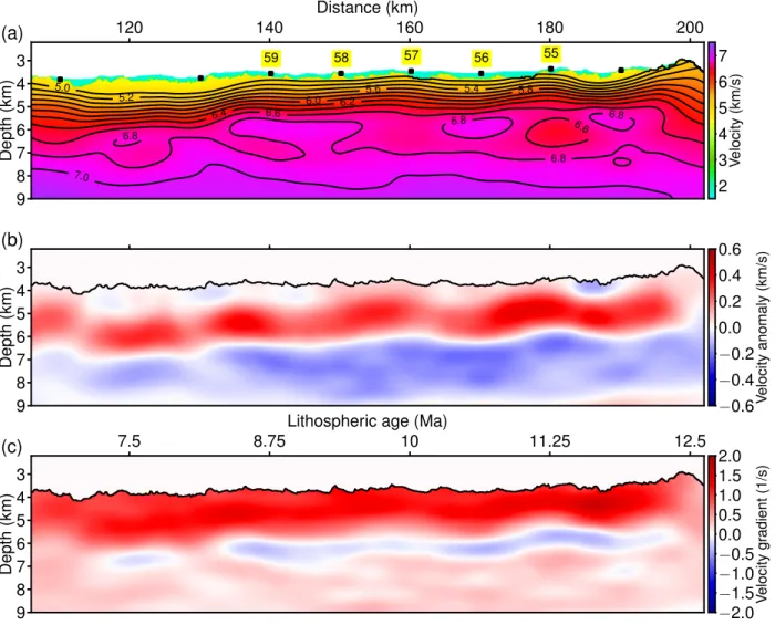
Fig. S3: Seismic images of the oceanic crust from the traced-normalised FWI: (a) The velocity model from the trace-normalised FWI, (b) the velocity anomaly (the difference between the velocity models from the FWI and the tomography), and (c) the vertical velocity gradient (the derivative of velocity with respect to depth). The lithospheric age is calculated using a spreading rate of 16 mm/year12. Black dots in (a) mark the locations of OBS. The velocity contours in (a) are from 5 to 7 km/s with an increment of 0.2 km/s. The coloured parts in (b) and (c) start from the basement (the top boundary of Layer 2). The horizontal distance starts with 0 km from the MAR. We invert the velocity model from FWI down to a maximum 9 km depth, because of potential Moho reflection interference for greater depths (Figs. S23, S24).
120 140 Distance (km)160 180 200
3 4 5 6 7 8 9
Depth(km)
56 55 58 57
59
(a)
5.0 5.2 5.6 5.4 5.8
6.0 6.2
6.4 6.6
6.6 6.8 6.8 6.8
6.8 7.0
7.03
4 5 6 7 8 9
Depth(km)
(b)
7.5 8.75Lithospheric age (Ma)10 11.25 12.5
3 4 5 6 7 8 9
Depth(km)
(c)
2 3 4 5 6 7
Velocity(km/s)
0.6 0.4 0.2 0.0 0.2 0.4 0.6
Velocityanomaly(km/s)
2.01.5 1.00.5 0.00.5 1.01.5 2.0
Velocitygradient(1/s)
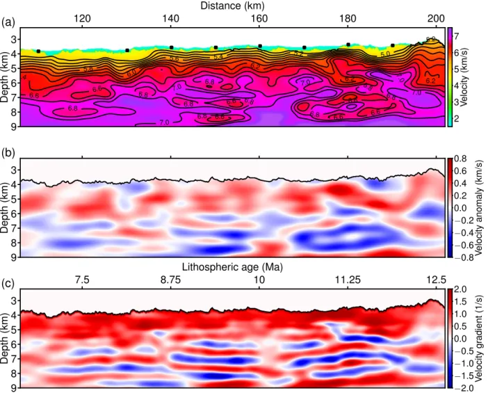
Fig. S4: Seismic images of the oceanic crust from the ‘true-amplitude’ FWI. (a) The velocity model from the ‘true-amplitude’ FWI, (b) the velocity anomaly (the difference between the velocity models from the FWI and the tomography), and (c) the vertical velocity gradient (the derivative of velocity with respect to depth). The lithospheric age is calculated using a spreading rate of 16 mm/year12. Black dots in (a) mark the locations of OBS. The velocity contours in (a) are from 5 to 7 km/s with an increment of 0.2 km/s. The coloured parts in (b) and (c) start from the basement (the top boundary of Layer 2). We invert the velocity model from FWI down to a maximum 9 km depth, because of potential Moho reflection interference for greater depths (Figs.
S23, S24).
120 140 Distance (km)160 180 200
3 4 5 6 7 8 9
Depth(km)
(a)
5.0
5.2 5.4 5.2
5.6
5.8 6.0
6.2
6.2 6.2 6.4
6.6 6.6
6.6 6.6
6.6 6.6 6.6
6.8
6.8 6.8
6.8
6.8 6.8
6.8 6.8
7.0 6.8
7.0
7.0
7.0 7.0 7.0
3 4 5 6 7 8 9
Depth(km)
(b)
7.5 8.75Lithospheric age (Ma)10 11.25 12.5
3 4 5 6 7 8 9
Depth(km)
(c)
2 3 4 5 6 7
Velocity(km/s)
0.8 0.6 0.4 0.2 0.0 0.2 0.4 0.6 0.8
Velocityanomaly(km/s)
2.0 1.5 1.0 0.5 0.0 0.5 1.0 1.5 2.0
Velocitygradient(1/s)
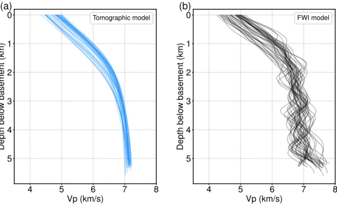
Fig. S5: Velocity-depth profiles: (a) One-dimensional velocity-depth profiles from the tomographic velocity model in Fig. 2a and (b) from the FWI model in Fig. S4a, between the distances from 112 km to 192 km at an increment of 2 km.
4 5 6 7 8
Vp (km/s) 0
1 2 3 4 5
Depthbelowbasement(km)
(a)
Tomographic model
4 5 6 7 8
Vp (km/s) 0
1 2 3 4 5
Depthbelowbasement(km)
(b)
FWI model
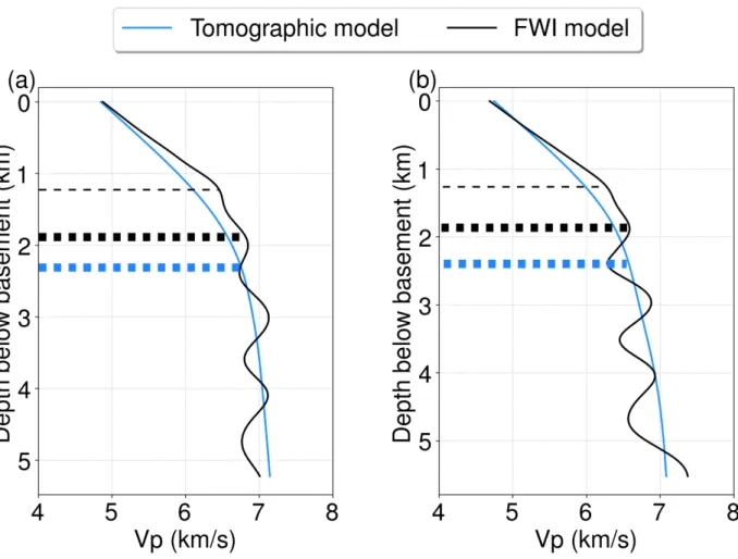
Fig. S6: Velocity-depth profiles: Two velocity profiles from the tomographic model in Fig. 2a and the FWI model in Fig. S4a, at distance (a) 146 km and (b) 182 km from the MAR,
respectively. The thin dashed line indicates the interpreted Layer 2A/2B boundary from FWI;
the bold dashed blue and black lines indicate the boundaries of Layer 2/3 from the tomographic model and the FWI model, respectively.
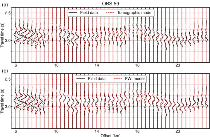
Fig. S7: Data comparison for OBS 59: (a) The recorded field data (black) and synthetic waveform (red) using the tomographic model (Fig. 2a), and (b) the recorded data (black) and synthetic waveform (red) using the true-amplitude FWI model (Fig. S4a). A reduced travel time of 7 km/s velocity was applied to both the field and synthetic data for plotting purpose.
6 10 14 18 23
2.5
3.0
Traveltime(s)
(a) OBS 59
Field data Tomographic model
6 10 14 18 23
Offset (km) 2.5
3.0
Traveltime(s)
(b)
Field data FWI model
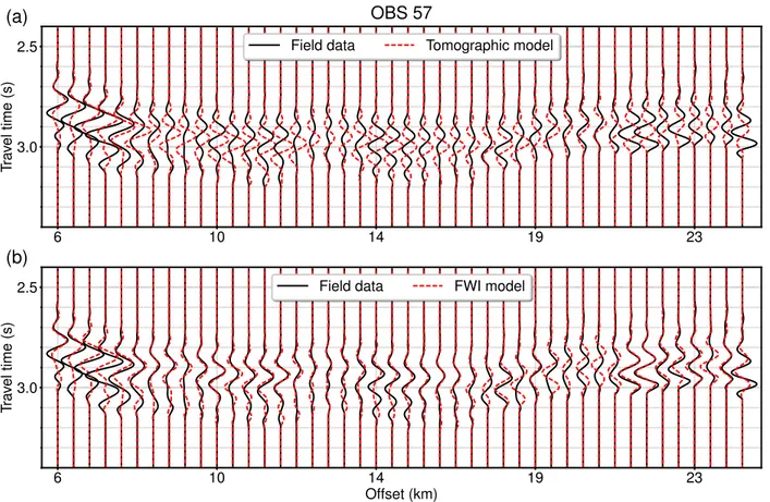
Fig. S8: Data comparison for OBS 57: (a) The recorded field data (black) and synthetic waveform (red) using the tomographic model (Fig. 2a), and (b) the recorded data (black) and synthetic waveform (red) using the true-amplitude FWI model (Fig. S4a). A reduced travel time of 7 km/s velocity was applied to both the field and synthetic data for plotting purpose.
6 10 14 19 23
2.5
3.0
Traveltime(s)
(a) OBS 57
Field data Tomographic model
6 10 14 19 23
Offset (km) 2.5
3.0
Traveltime(s)
(b)
Field data FWI model
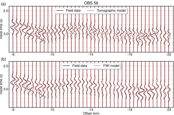
Fig. S9: Data comparison for OBS 56: (a) The recorded field data (black) and synthetic waveform (red) using the tomographic model (Fig. 2a), and (b) the recorded data (black) and synthetic waveform (red) using the true-amplitude FWI model (Fig. S4a). A reduced travel time of 7 km/s velocity was applied to both the field and synthetic data for plotting purpose.
-6 -10 -14 -19 -23
2.5
3.0
Traveltime(s)
(a) OBS 56
Field data Tomographic model
-6 -10 -14 -19 -23
Offset (km) 2.5
3.0
Traveltime(s)
(b)
Field data FWI model
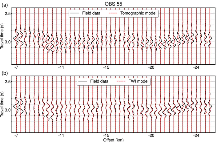
Fig. S10: Data comparison for OBS 55: (a) The recorded field data (black) and synthetic waveform (red) using the tomographic model (Fig. 2a), and (b) the recorded data (black) and synthetic waveform (red) using the true-amplitude FWI model (Fig. S4a). A reduced travel time of 7 km/s velocity was applied to both the field and synthetic data for plotting purpose.
-7 -11 -15 -20 -24
2.5
3.0
Traveltime(s)
(a) OBS 55
Field data Tomographic model
-7 -11 -15 -20 -24
Offset (km) 2.5
3.0
Traveltime(s)
(b)
Field data FWI model
120 140 Distance (km)160 180 200
3 4 5 6 7 8 9
Depth(km) 5.0
5.2 5.4 5.2
5.6
5.8 6.0
6.2 6.4 6.2
6.6 6.8 6.8 6.8
7.07.0 7.0 7.0
2 3 4 5 6 7
Velocity(km/s)
Fig. S11: Modified background velocity model: The layered structures in the lower crust from 5.8 km depth in the velocity model from the FWI (Fig. S4a) were removed and replaced by the corresponding tomographic model (Fig. 2a) for synthetic FWI studies. This altered model was used as a starting model for various FWI tests (Figs. S12, S16-S20).
Fig. S12: Model recovery test: Seismic images of the oceanic crust from the FWI using the altered model (Fig. S10) as the starting model. (a) The inverted velocity model from the FWI, (b) the velocity anomaly (the difference between the velocity model from the FWI and the
tomography), and (c) the vertical velocity gradient (the derivative of velocity with respect to depth). The recovered seismic images of the oceanic crust are very similar to those in Fig. S4.
120 140 Distance (km)160 180 200
3 4 5 6 7 8 9
Depth(km)
(a)
5.0
5.2
5.2 5.4
5.6 5.8
6.0 6.2
6.4 6.4
6.6 6.6
6.6
6.8 6.8 6.8
6.8
6.8 6.8
7.0
7.0 7.0
7.0
7.0 7.0
7.0
3 4 5 6 7 8 9
Depth(km)
(b)
7.5 8.75Lithospheric age (Ma)10 11.25 12.5
3 4 5 6 7 8 9
Depth(km)
(c)
2 3 4 5 6 7
Velocity(km/s)
0.8 0.6 0.4 0.2 0.0 0.2 0.4 0.6 0.8
Velocityanomaly(km/s)
2.0 1.5 1.0 0.5 0.0 0.5 1.0 1.5 2.0
Velocitygradient(1/s)
Fig. S13: Model recovery test data comparison: (a) Comparison between the field data (black) and the synthetic data (red) from the altered model (Fig. S11). (b) Comparison between the field data (black) and the synthetic data (red) using the model from the FWI using the altered model (Fig. S11) as the starting model.
7 11 15 20 24
2.5
3.0
Traveltime(s)
(a) OBS 58
Field data After removing layering
7 11 15 20 24
Offset (km) 2.5
3.0
Traveltime(s)
(b)
Field data FWI model
Fig. S14: Checkerboard test 1: The checkerboard model 1 was generated by adding 8%
positive and negative Gaussian-shape velocity anomalies to the tomographic velocity model.
Each of the anomalies has 10 km lateral extension and 1 km thickness. (a) The true checkerboard velocity perturbation, and (b) the recovered velocity anomalies from the FWI.
120 140 Distance (km)160 180 200
3 4 5 6 7 8 9
Depth(km)
(a)
3 4 5 6 7 8 9
Depth(km)
(b)
0.6 0.4 0.2 0.0 0.2 0.4 0.6
Velocityanomaly(km/s)
0.6 0.4 0.2 0.0 0.2 0.4 0.6
Velocityanomaly(km/s)
Fig. S15: Checkerboard test 2: The checkerboard model 2 was generated by adding 8%
positive and negative Gaussian-shape velocity anomalies to the tomographic velocity model.
Each of the anomalies has 10 km lateral extension and 0.5 km thickness. (a) The true
checkerboard velocity perturbation, and (b) the recovered velocity anomalies from the FWI.
120 140 Distance (km)160 180 200
3 4 5 6 7 8 9
Depth(km)
(a)
3 4 5 6 7 8 9
Depth(km)
(b)
0.6 0.4 0.2 0.0 0.2 0.4 0.6
Velocityanomaly(km/s)
0.6 0.4 0.2 0.0 0.2 0.4 0.6
Velocityanomaly(km/s)
Fig. S16: Layered model resolution test: The model in Fig. S11 was perturbed by adding the alternating high- and low- velocity layers in (a). The layers are 500 m thick with the velocity anomalies of ±200 m/s. (b) Starting with the unperturbed model (Fig. S11), the velocity anomalies recovered by FWI.
120 140 Distance (km)160 180 200
3 4 5 6 7 8 9
Depth(km)
(a)
3 4 5 6 7 8 9
Depth(km)
(b)
0.20 0.15 0.10 0.05 0.00 0.05 0.10 0.15 0.20
Velocityanomaly(km/s)
0.20 0.15 0.10 0.05 0.00 0.05 0.10 0.15 0.20
Velocityanomaly(km/s)
Fig. S17: Gradient layered model resolution test: The model in Fig. S11 was perturbed by adding the alternating high- and low- velocity layers in (a). The layers are 500 m thick with the velocity anomalies of maximum ±200 m/s, with a gradient of 1 s-1. (b) Starting with the
unperturbed model (Fig. S11), the velocity anomalies recovered by FWI.
120 140 Distance (km)160 180 200
3 4 5 6 7 8 9
Depth(km)
(a)
3 4 5 6 7 8 9
Depth(km)
(b)
0.20 0.15 0.10 0.05 0.00 0.05 0.10 0.15 0.20
Velocityanomaly(km/s)
0.20 0.15 0.10 0.05 0.00 0.05 0.10 0.15 0.20
Velocityanomaly(km/s)
Fig. S18: Gradational layering model resolution test: The model in Fig. S11 was perturbed by adding the gradational-varying layers in (a). The gradational layers are 500 m thick where the velocity increases linearly by + 350 m/s and then sharply decreases to the background velocity at its base. (b) Starting with the unperturbed model (Fig. S11), the velocity anomalies recovered by FWI.
120 140 Distance (km)160 180 200
3 4 5 6 7 8 9
Depth(km)
(a)
3 4 5 6 7 8 9
Depth(km)
(b)
0.3 0.2 0.1 0.0 0.1 0.2 0.3
Velocityanomaly(km/s)
0.3 0.2 0.1 0.0 0.1 0.2 0.3
Velocityanomaly(km/s)
120 140 Distance (km)160 180 200
3 4 5 6 7 8 9
Depth(km)
(a)
3 4 5 6 7 8 9
Depth(km)
(b)
0.6 0.4 0.2 0.0 0.2 0.4 0.6
Velocityanomaly(km/s)
0.6 0.4 0.2 0.0 0.2 0.4 0.6
Velocityanomaly(km/s)
Fig. S19: Step-wise increasing-velocity layering model resolution test: The model in Fig. S11 was perturbed by adding the step-wise increasing velocity layers in (a). Each of the velocity anomaly layer is 500 m thick with a velocity increase of 200 m/s from its shallower neighboring layer. (b) Starting with the unperturbed model (Fig. S11), the velocity anomalies recovered by FWI.
Fig. S20: Layered model resolution test: The model in Fig. S11 was perturbed by adding a low-velocity layer in (a). The layer is 400 m thick with velocity anomalies of maximum ±300 m/s and a Gaussian-shape transition. (b) Starting with the unperturbed model (Fig. S11), the velocity anomalies recovered by FWI.
120 140 Distance (km)160 180 200
3 4 5 6 7 8 9
Depth(km)
(a)
3 4 5 6 7 8 9
Depth(km)
(b)
0.3 0.2 0.1 0.0 0.1 0.2 0.3
Velocityanomaly(km/s)
0.3 0.2 0.1 0.0 0.1 0.2 0.3
Velocityanomaly(km/s)
Fig. S21: One-dimensional velocity profiles for layering model synthetic studies: Velocity- depth functions at the distance of 168 km for the unperturbed (the initial model for FWI, blue), the true (red) and inverted models (black), for (a) the layered model, (b) the gradient layered model, (c) the gradational layering model, (d) the step-wise increasing-velocity layering model, and (e) a low-velocity anomaly model.
6.5 7.0 7.5 8.0 Vp (km/s) 5
6
7
8
9
Depth(km)
(a)
Starting model True model FWI
6.5 7.0 7.5 8.0 Vp (km/s) (b)
6.5 7.0 7.5 8.0 Vp (km/s) (c)
6.5 7.0 7.5 8.0 Vp (km/s) (d)
6.5 7.0 7.5 8.0 Vp (km/s) (e)
120 140 160 180 200
Distance (km)
34 5 67 89 1011
Depth(km)
(a)
5.000 5.600 5.400 5.200
5.800 6.000 6.200
6.400 6.600
6.800
7.000
7.200 7.400 7.600 7.800
8.000
34 56 78 109 11
Depth(km)
(b)
5.000 5.600 5.800 5.400 5.200
6.000 6.200
6.400 6.600
6.800
7.000
7.000
7.200 7.200 7.200 7.200 7.200
2 3 4 5 6 7 8
Velocity(km/s)
2 3 4 5 6 7 8
Velocity(km/s)
Fig. S22: Moho reflection interference test: (a) The velocity model12 from travel-time tomography with Moho and upper mantle included was used as the ‘true’ model for generating
‘observed’ seismic data for FWI; (b) the same velocity model with (a) after removing the Moho and upper mantle (the velocities of these parts were replaced by velocities immediately above the Moho) was used as the starting velocity model for FWI.
Fig. S23: Seismic images from FWI for the Moho interference test 1: (a) The velocity model from FWI, (b) the velocity anomaly (the difference between the velocity model from the FWI and the starting model), and (c) the vertical velocity gradient (the derivative of velocity with
120 140 Distance (km)160 180 200
34 56 78 109 11
Depth(km)
(a)
5.000 5.200
5.400
5.600 6.200 6.000 5.800 6.400
6.600 6.800
7.000
7.000 7.000
7.000
7.000 7.000 7.000
7.000 7.200
7.200
7.200
7.200 7.200
7.400 7.400
7.600
34 56 78 109 11
Depth(km)
(b)
7.5 8.75Lithospheric age (Ma)10 11.25 12.5
34 56 78 109 11
Depth(km)
(c)
2 3 4 5 6 7 8
Velocity(km/s)
0.8 0.6 0.4 0.2 0.0 0.2 0.4 0.6 0.8
Velocityanomaly(km/s)
2.0 1.5 1.0 0.5 0.0 0.5 1.0 1.5 2.0
Velocitygradient(1/s)
respect to depth). The velocity contours in (a) are from 5 to 7 km/s with an increment of 0.2 km/s. FWI was performed using the same source and receiver positions and frequency ranges of the data as in the actual observation, and the same inversion parameters. The only difference is that a larger time window, i.e., between 0.2 s before, and 0.5 s after the picked Pg travel times, than that for field data FWI, was used for including both Pg and PmP arrivals in the ‘observed’
data for inversion.
Fig. S24: Seismic images from FWI for the Moho interference test 2: (a) The velocity model from FWI, (b) the velocity anomaly (the difference between the velocity model from the FWI and the starting model), and (c) the vertical velocity gradient (the derivative of velocity with
120 140 Distance (km)160 180 200
34 56 78 109 11
Depth(km)
(a)
5.000 5.200 5.400
5.600 5.800 6.000 6.200
6.400 6.600
6.800
7.000 7.200
7.200
7.200
7.200
7.200 7.200
7.200 7.200
7.400 7.400
34 56 78 109 11
Depth(km)
(b)
7.5 8.75Lithospheric age (Ma)10 11.25 12.5
34 56 78 109 11
Depth(km)
(c)
2 3 4 5 6 7 8
Velocity(km/s)
0.8 0.6 0.4 0.2 0.0 0.2 0.4 0.6 0.8
Velocityanomaly(km/s)
2.0 1.5 1.0 0.5 0.0 0.5 1.0 1.5 2.0
Velocitygradient(1/s)
respect to depth). The velocity contours in (a) are from 5 to 7 km/s with an increment of 0.2 km/s. FWI was performed using the same source and receiver positions and frequency ranges of the data as in the actual observation, and the same inversion parameters. The same size window as for field data FWI, was used for including mainly Pg arrivals and reducing the influence of PmP from the ‘observed’ data for inversion.
Physical properties Olivine (Ol) Clinopyroxene
(Cpx) Plagioclase (Pl)
Bulk moduli (GPa) 129.2 107.8 55.1
Shear moduli (GPa) 81.2 75.7 29.7
Density (g/cm3) 3.23 3.20 2.61
Table S1. Physical properties of Ol, Cpx and Pl from [Sobolev and Babeyko 1994].
Olivine (Ol)
Clinopyroxene
(Cpx) Plagioclase (Pl) Vp (km/s)
Olivine-rich gabbro: I 0.25 0.25 0.5 7.072
Olivine-rich gabbro: II 0.2 0.3 0.5 7.050
Olivine gabbro: I 0.15 0.3 0.55 6.934
Olivine gabbro: II 0.1 0.3 0.6 6.818
Olivine gabbro: III 0.1 0.4 0.5 7.005
Olivine-bearing
gabbro: I 0.05 0.3 0.65 6.703
Olivine-bearing
gabbro: II 0.05 0.25 0.7 6.611
Table S2: The effective P-wave velocities from VRH averaging using different fraction volumes of mineral components (Ol, Cpx and Pl).