The ATLAS Collaboration

ATLAS-CONF-2017-062 24July2017

ATLAS CONF Note

ATLAS-CONF-2017-062

18th July 2017

Jet reclustering and close-by effects in ATLAS Run 2

The ATLAS Collaboration

The reconstruction of hadronically-decaying, high- p

W , Z and Higgs bosons and top quarks is instrumental to exploit the physics potential of the ATLAS detector in pp collisions at a centre-of-mass energy of 13 TeV at the Large Hadron Collider (LHC). The jet reclustering procedure reconstructs such objects by using calibrated anti- k

jets as inputs to the anti- k

algorithm with a larger distance parameter. The performance of these reclustered large-radius jets during LHC Run 2 is studied, and compared with that of trimmed anti- k

large-radius jets directly constructed from locally calibrated topological clusters. The propagation of calibrations to reclustered jets is found to be sufficient to restore their average energy and mass scales to particle level. The modelling of small-radius anti- k

jets in each other’s vicinity is studied using methods which combine tracking and calorimeter information. Systematic uncertainties resulting from the propagation of the uncertainties on the input jets to the reclustering procedure are studied. Comparisons between 33.2 fb

of data collected during 2016 operations and simulation are shown, and the relative jet mass scale and resolution for reclustered and conventional jets are extracted using the forward-folding technique.

© 2017 CERN for the benefit of the ATLAS Collaboration.

Reproduction of this article or parts of it is allowed as specified in the CC-BY-4.0 license.

1 Introduction

The shower of particles originating from the hadronisation and fragmentation of a strongly-interacting particle produced in a high-energy particle collision is reconstructed experimentally as a jet. At the Large Hadron Collider (LHC), jets are reconstructed using recombination procedures [1, 2] such as the anti- k

algorithm [3], Cambridge-Aachen algorithm [4, 5] and k

algorithm [6, 7]. Jets may be built using a collection of four-vectors which corresponds to a set of simulated particles, tracks of charged particles in the inner detector (section 2), or calibrated topological clusters built from energy depositions in the calorimeter [8]. Recombination algorithms accept one user-determined distance parameter, R , which determines the ultimate size of the output jets. Jets built from topological clusters using the anti- k

algorithm and R = 0 . 4 are widely-used by ATLAS, and are supported by a complex energy- and mass-calibration procedure and corresponding suite of systematic uncertainties [9]. ‘Conventional’

large- R anti- k

jets built directly from calorimeter clusters with R = 1 . 0 are also supported with their own dedicated energy and mass calibrations and uncertainties [10], and are often used to reconstruct high-transverse-momentum (high- p

), hadronically-decaying W , Z and Higgs bosons and top quarks (“boosted” bosons and top quarks).

The use of calibrated, small- R jets as inputs to large- R jet reconstruction has been applied in many ATLAS searches for supersymmetry (SUSY) [11–17] and exotica [18–20] throughout Runs 1 and 2 of the LHC.

This procedure, known as jet reclustering [21], propagates calibrations and uncertainties from the input jets through to the final large- R jets, exploiting our detailed understanding of the input objects in order to provide greater flexibility at the physics analysis level. The performance of reclustered and conventional large- R jets is directly compared in these studies.

The propagation of calibrations and uncertainties to reclustered jets eliminates the need to prepare a specific calibration for the large- R jets considered for use in the final data analysis. This allows individual searches and measurements to optimise the large- R jet distance parameter and the details of the grooming procedure, i.e., the dedicated algorithm to remove soft and collinear radiation from jets, provided that the input jets used for reclustering are themselves not modified. As only specific large- R jet sizes and grooming configurations are supported by ATLAS (currently, only anti- k

R = 1 . 0 jets trimmed with f

=5% and R

=0.2 [10, 22]), this can lead to large gains in analysis sensitivity depending on the final state in question. When searching for high-mass resonances or massive supersymmetric particles decaying into high- p

W , Z and Higgs bosons and top quarks, a jet built with R = 1 . 0 may not always be optimal. Reclustered jets with radii as small as R = 0 . 8 and as large as R = 1 . 4 have been previously used in ATLAS searches. Some care must be taken when discussing the finer details of jet substructure in the context of reclustered jets, particularly when defining observables which are sensitive to soft radiation within a large- R jet, such as the N -subjettiness [23, 24]. As such, a discussion of substructure observables other than the calorimeter-based jet mass is beyond the scope of the studies presented here.

The calibrations and uncertainties applied to the anti- k

R = 0 . 4 jets used as inputs when reclustering are based on analyses of well-understood, isolated systems of dijet, multijet, γ +jet and Z +jet systems [9].

As these systems do not contain large amounts of additional activity near the selected jets, it is possible

that calibrations and uncertainties derived in these topologies will break down as the amount of radiation

(hadronic activity) near a jet increases. As dense systems of many close-by jets are often reclustered

when reconstructing a massive hadronically decaying particle, it is necessary to understand these potential

limitations. The applicability of jet calibrations intended for a single jet on this merged object in the

proximity of additional radiation was previously unclear, and is a focal point of the studies presented

here.

Figure 1 provides a specific example of a scenario where close-by effects may be important to consider, for the case of boosted top quarks. A toy two-step decay chain with scalar particles X → Y Z(→ AB) illustrates the qualitative behavior similar to a boosted top quark, since m

= 175 GeV ≈ m

, m

= 80 GeV ≈ m

and m

= m

= m

= 0. The top-quark-like particle X is in a fully resolved regime when all of the particles are further apart than the small-radius jet radius, R = 0 . 4. As the transverse momentum of the mother particle X increases, the number of decay products which are separated by more than ∆R = 0 . 4 decreases. For intermediate values of p

(600-1200 GeV), two of the three particles produced by the decay of particle X are likely to have merged into a single ∆R = 0 . 4 region (‘jet’) with significant mass which is also usually within ∆R < 1 . 0 of the remaining parton.

This note is a collection of studies associated with the procedure of jet reclustering in ATLAS, performed during 2016 datataking at the LHC. A brief overview of the ATLAS detector is provided in section 2, and a summary of the data and simulated event samples used in the various studies is provided in section 3. Section 4 details the general performance of reclustered large- R jets and draws comparisons with conventional trimmed anti- k

large- R jets directly constructed from topological clusters. Section 5 presents studies of the modelling of jets in the vicinity of nearby radiation. A breakdown of the effects of systematic uncertainties propagated from the input jets to reclustered jets is shown in section 6.

Comparisons between data and simulation, and other in situ studies are shown in section 7.

2 The ATLAS detector

ATLAS1 is a cylindrical, multi-purpose detector with nearly 4 π coverage in solid angle, built around interaction point 1 of the LHC at CERN [25]. The inner detector (ID) provides measurements of charged particle momenta up to psuedorapiditites of |η | < 2 . 5 using silicon pixel and microstrip detectors. A transition radiation tracking (TRT) detector provides enhanced electron identification capabilities within

|η| < 2 . 0. A thin superconducting solenoid surrounds the ID, immersing it within a constant 2 T axial magnetic field.

The ATLAS electromagnetic calorimeter resides between the solenoid and its cryostat vessel wall. It utilises lead absorbing and liquid argon sampling layers to contain and measure showers of particles occurring within pseudorapidities of |η| < 3 . 2, at depths between 24 – 27 radiation lengths ( X

). Beyond the cryostat vessel wall, the ATLAS scintillating-tile/steel hadronic tile calorimeter provides energy measurement and shower containment for hadronic activity within |η | < 1 . 7. The end-cap regions (1 . 5 < |η| < 3 . 2) of the detector are instrumented with liquid argon calorimeters with either stainless steel or copper absorbing layers, respectively in the electromagnetic and hadronic endcap calorimeter modules (EMEC, HEC). The forward calorimeter provides both electromagnetic and hadronic energy measurements beyond the coverage of the EMEC and HEC, extending coverage from |η | > 3 . 2 to |η < 4 . 9 | with liquid argon systems utilising either copper or tungsten absorbers, depending on the calorimeter layer.

Altogether, the combined ATLAS calorimetry systems provide containment for hadronic activity to shower depths greater than 10 hadronic interaction lengths ( λ

) across nearly the entire detector acceptance (up to |η| < 4 . 9).

1ATLAS uses a right-handed coordinate system with its origin at the nominal interaction point (IP) in the centre of the detector and thez-axis along the beam pipe. The x-axis points from the IP to the centre of the LHC ring, and the y-axis points upward. Cylindrical coordinates(r, φ)are used in the transverse plane,φbeing the azimuthal angle around thez-axis. The pseudorapidity is defined in terms of the polar angleθasη=−ln tan(θ/2).

[GeV]

X

pT

0 200 400 600 800 1000 1200 1400

Fraction of Events

0 0.2 0.4 0.6 0.8 1 1.2 1.4

R(all parton pairs) > 1.0 (resolved)

∆

R(pair) < 1.0

∆ R(all parton pairs) > 0.4 and at least one

∆

R(pair) < 0.4

∆ R(pair) < 1.0 and exactly one

∆ At least one

R(all parton pairs) < 0.4 (merged)

∆

C D)

→ A B (

→ Toy MC, X

D = 0

C = m

A = m = 80 GeV, m = 175 GeV, mB

mX

partons: A, C, D for simplicity, all particles are scalars

Figure 1: A scalar particle (X) decays to two particles AandB. The particleBsubsequently decays into particles CandD. To resemble a boosted top decay,mX=175 GeV≈m_t(the mass of the top quark),mB=80 GeV≈mW

(the mass of theW boson), andm_A=m_C =m_D=0. Plotted is the fraction of events that are resolved, merged and in-between resolved and merged, as a function ofp_Tof particleX. The intermediate regime in which reclustering interpolates between single and multiple resolved jets is shown as the broken black distribution: in this region, close-by effects are important to consider as there is a massive small-radius jet very close to another jet. The intermediate regime before the dashed line has all three particles close enough to form one large-radius jet, but still sufficiently far apart that three small-radius jets are resolved inside the large-radius jet.

The ATLAS muon spectrometer is rigged around the tile calorimeter, and contains the three air-cored superconducting toroidal magnets after which ATLAS is named. Three layers of tracking chambers allow the full muon momentum to be reconstructed up to pseudorapidities inside of |η| < 2 . 7, and separate, dedicated chambers with a faster readout time allow triggering on muons within |η| < 2 . 4.

The ATLAS trigger system [26] consists of a hardware-based Level-1 system, which reduces the rate of event collection from up to 40 MHz to 100 kHz; and a software-based high level trigger (HLT), which processes events in order to further reduce the rate to 1 kHz. Events passing selection in the HLT are written to disk for use in analysis.

3 Data and simulation

The data presented within this note were collected during 2016 operation of the LHC, corresponding to

an integrated luminosity of 33.2 fb

following data quality requirements. During data-taking in 2016,

the average number of interactions per bunch crossing was 24.9 and the proton bunch spacing in the LHC was 25 ns. In section 5, a chain of single-jet triggers selects dijet and multijet events with leading-jet transverse momenta as low as 220 GeV, in which the effects of close-by radiation on jet modelling is studied. Within the analysis presented in section 7, t t ¯ events in the lepton+jets channel are selected using single-muon triggers, which are fully efficient following a requirement that reconstructed muons in these events have a p

> 25 GeV. These events provide a convenient environment to study the properties of high- p

, hadronically decaying W bosons and top quarks in situ .

Studies documented within this note are performed using a variety of Monte Carlo (MC) simulated samples produced by ATLAS. Dijet events are generated at LO in Pythia 8.1 [27] with the 2 → 2 matrix element convolved with the NNPDF2.3LO PDF set [28] and using the A14 event tune [29]. The parton shower and fragmentation is simulated in Pythia 8.1 using the leading-logarithmic approximation through p

-ordered parton showers [30]. Additional dijet events are simulated using different generators, in order to provide several comparisions to data when studying the effects of close-by radiation on jets. Sherpa 2.1 [31]

generates events using multi-leg 2 → N matrix elements, which are matched to parton showers following the CKKW prescription [32]. These Sherpa events are simulated using the CT10 PDF set [33] and default Sherpa event tune. Herwig++ 2.7 [34, 35] provides a sample of events where additional radiation is showered using angular-ordering. These events are generated with the 2 → 2 matrix element, convolved with the CTEQ6L1PDF set [36] and configured with the UE-EE-5 tune [37].

In order to study the resolution of jet reclustering in boosted W boson and top quark topologies, exotic W

and Z

bosons with a wide range of masses (from 400 GeV to 5 TeV) are simulated using Pythia 8.1, then forced to decay hadronically, respectively through W and Z bosons or top quarks2. This approach provides a source of boosted objects across a wide range of p

for study.

For the in situ studies presented in section 7, several additional samples of Standard Model physics processes are used. The details of the t t ¯ and single top [38], W/Z +jets [39] and diboson [40] samples which are included in these studies may be found in their respective references.

All simulated events have been reconstructed using a full simulation of the ATLAS detector [41] imple- mented in Geant 4 [42], which describes the interactions of particles with the detector. Hadronic showers are simulated using the FTFP BERT model [43]. The effects of multiple simultaneous pp collisions (pileup) are simulated with unbiased pp collisions using Pythia 8.1 and overlaid on the nominal dijet interactions.

4 MC-based performance

The response of a jet observable such as its transverse momentum ( p

) or mass ( m ) is defined as the ratio of the calorimeter jet observable to that of the associated jet at particle-level, reconstructed with the same jet algorithm:

R

T

= p

T

p

T

, (1)

R

= m

m

. (2)

2The requirement on hadronic decays is enforced during sample generation for theW⁰samples and at the analysis level for the Z⁰samples.

Following calibration, the average response of a reconstructed jet observable for an ensemble of jets should be restored to its average particle-level value. As the input anti- k

R = 0 . 4 jets have already been calibrated, the large- R jet produced should also be calibrated. Any deviation of the average response value from that at particle-level following calibration is referred to as “non-closure,” and could be indicative that additional calibration is necessary. The closures of reclustered jets are compared to those of conventional, trimmed anti- k

R = 1 . 0 jets built directly from topological clusters, in the dijet topologies which are used to create the calibrations applied to both the small- R and conventional large- R jets.

Conventional ATLAS large- R jets are built directly from topological clusters calibrated at the local hadronic scale [8]. Large- R jets and their substructure are susceptible to the effects of pile-up contamination3, and so these jets are trimmed by reclustering their input constituents using the k

algorithm with a distance parameter of R

= 0 . 2, then discarding any of the k

sub-jets which fail to possess at least 5% of the original jet’s transverse momentum ( f

= 0 . 05) [22]. This procedure also improves the mass resolution of large- R jets which reconstruct massive objects, and improves the signal/background performance of the widely-used electroweak boson and top tagging techniques which rely on the jet mass for discrimination power.

Reclustered jets are built from anti- k

R = 0 . 4 jets with at least 25 GeV of transverse momentum and

|η| < 2 . 5, built from topological clusters which have been calibrated at the electromagnetic scale [8, 45].

Reconstructed jets are calibrated to particle-level through the application of a jet energy scale calibration (JES) derived from

√ s = 13 TeV collision data and simulation, a global sequential calibration (GSC) used to improve the resolution and flavour response [9], and a jet mass scale calibration (JMS) which is derived using simulated dijet events. These calibrated small- R jets are used as inputs to the anti- k

algorithm with R = 1 . 0 in order to produce large- R reclustered jets. To follow the procedure applied to standard large- R jets in ATLAS, these reclustered jets are also trimmed by discarding any constituents (here, the input small- R jets) which fail to possess at least 5% of the untrimmed reclustered jet’s transverse momentum4. The choice of the trimming f

parameter is also based on the value selected in previous ATLAS results [16, 17]. No additional calibration is applied to the energy or mass of these new objects.

Truth jets are built from particle four-vectors obtained directly from the Monte Carlo generator, before the ATLAS detector simulation is applied. Only the subset of these particles which are stable within the ATLAS detector and which may leave a significant deposition of energy in the calorimeter (particles with cτ > 10 mm which are not muons or neutrinos) are selected for truth jet reconstruction. These stable particles are given as inputs to the anti- k

algorithm with a distance parameter of either R = 1 . 0 or R = 0 . 4, to produce large- and small- R truth jets. Large- R truth jets are trimmed using the same procedure as the conventional, reconstructed large- R jets and matched to these directly using the criterion that the angular separation ( ∆R ) between the large- R reconstructed and truth jet be less than 0 . 6 ( ∆R < 0 . 6).

The R = 0 . 4 truth jets are matched within ∆R < 0 . 3 to the reconstructed small- R jets which form the constituents of large- R reclustered jets. These matched small- R truth jets are used to build ‘reclustered’

truth jets: the four-vectors of all truth jets matched to constituents of reclustered jets are summed in order to obtain a four-vector which represents the full set of input jets for each reclustered jet. This approach guarantees that the number of reconstructed and truth jet constituents associated with reclustered jets will never differ, which in turn ensures that the jet response will appropriately describe the p

or mass of the jet in question. Events for which the reclustered jet does not include a matched truth-level jet for each reconstructed jet are not considered in these studies. All reclustered and conventional large- R jets are

3The amount of pileup contamination which may impact a jet scales as the square of the distance parameterRwhich is used to reconstruct the jet [44].

4Note that thep_Tthreshold on the input jets acts as an effective trimming as well.

required to be well-isolated at both truth- and detector-level: large- R jets with another large- R truth jet or large- R reconstructed jet within ∆R < 2 . 5 satisfying p

> 150 GeV and |η| < 2 . 0 are not selected for modelling studies. Truth jets may be matched with W bosons or top quark jets by requiring that the truth jet is matched to within ∆R < 0 . 75 of a hadronically-decaying W boson or top quark at parton-level [46].

Response distributions for both conventional and reclustered large- R jets are produced, then their cores are fit with a Gaussian distribution in the range of ± 2 σ around the peak of the distribution. The fitted position of the Gaussian peak is shown as a function of p

T

and m

in figures 2 and 3 for representative kinematic regions. Good closure is observed for both reclustered and conventional large- R jets in dijet topologies, except occasionally at low jet masses. As the performance of reclustered large- R jets is consistent with that of conventional large- R jets, it may be concluded that the propagation of energy and mass calibrations from the input objects when reclustering is sufficient to restore the average p

and mass values of reclustered jets to their particle-level quantities, and that additional calibration of the large- R reclustered objects is not necessary.

The large- R jet calorimeter mass resolution, defined as the 68% inter-quantile range of the response distribution divided by twice the median of the response distribution5, is shown in Figure 4 as a function of the truth jet transverse momentum. The mass resolution is shown for high- p

W bosons and top quarks, which produce jets with substantial mass, which may in turn be used to differentiate these jets from other large- R jets produced by light quarks and gluons [46, 47]. A smaller mass resolution implies increased performance when attempting to reconstruct and identify the origin of these objects. Reclustered jets are observed to have a smaller calorimeter mass resolution than conventional trimmed large- R jets for both W and top jets, across nearly the entire examined p

range. This improvement is likely attributable to the separate calibration of each input constituent used to produce reclustered jets, and may be as much as 22% for boosted W bosons and 29% for boosted top quarks within a representative kinematic region ( |η| < 0 . 4). The large- R jet track-assisted mass [10] is not considered for comparison in these studies, as track-based augmentation of the input anti- k

R = 0 . 4 jets used in jet reclustering is unavailable at this time.

5If a jet response distribution is perfectly Gaussian, this measure of resolution simplifies to the ratio of the Gaussian standard deviation to mean of the distribution.

[GeV]

true

pT

200 400 600 800 1000 1200 1400 1600 1800 2000

〉 T

true / p T

reco p〈

0.9 0.95 1 1.05

1.1

ATLAS Simulation Preliminary

| < 0.4 η 13 TeV, Pythia 8 dijets; |

R=1.0 LC+JES+JMS jets

=0.2) anti-kt

=5%, Rsub

Trimmed (fcut

R=0.4 EM+JES+GSC+JMS jets

=5%) jets from anti-kt

Reclustered (R=1.0, fcut

Trimmed, R=1.0 < 60 GeV 40 GeV < mtrue

< 100 GeV 80 GeV < mtrue

< 200 GeV 160 GeV < mtrue

Reclustered, R=1.0 < 60 GeV 40 GeV < mtrue

< 100 GeV 80 GeV < mtrue

< 200 GeV 160 GeV < mtrue

ATLAS Simulation Preliminary

| < 0.4 η 13 TeV, Pythia 8 dijets; |

R=1.0 LC+JES+JMS jets

=0.2) anti-kt

=5%, Rsub

Trimmed (fcut

R=0.4 EM+JES+GSC+JMS jets

=5%) jets from anti-kt

Reclustered (R=1.0, fcut

Trimmed, R=1.0 < 60 GeV 40 GeV < mtrue

< 100 GeV 80 GeV < mtrue

< 200 GeV 160 GeV < mtrue

Reclustered, R=1.0 < 60 GeV 40 GeV < mtrue

< 100 GeV 80 GeV < mtrue

< 200 GeV 160 GeV < mtrue

ATLAS Simulation Preliminary

| < 0.4 η 13 TeV, Pythia 8 dijets; |

R=1.0 LC+JES+JMS jets

=0.2) anti-kt

=5%, Rsub

Trimmed (fcut

R=0.4 EM+JES+GSC+JMS jets

=5%) jets from anti-kt

Reclustered (R=1.0, fcut

(a)

[GeV]

true

pT

200 400 600 800 1000 1200 1400 1600 1800 2000

〉true / mreco m〈

0.9 0.95 1 1.05

1.1

ATLAS Simulation Preliminary

| < 0.4 η 13 TeV, Pythia 8 dijets; |

R=1.0 LC+JES+JMS jets

=0.2) anti-kt

=5%, Rsub

Trimmed (fcut

R=0.4 EM+JES+GSC+JMS jets

=5%) jets from anti-kt

Reclustered (R=1.0, fcut

Trimmed, R=1.0 < 60 GeV 40 GeV < mtrue

< 100 GeV 80 GeV < mtrue

< 200 GeV 160 GeV < mtrue

Reclustered, R=1.0 < 60 GeV 40 GeV < mtrue

< 100 GeV 80 GeV < mtrue

< 200 GeV 160 GeV < mtrue

ATLAS Simulation Preliminary

| < 0.4 η 13 TeV, Pythia 8 dijets; |

R=1.0 LC+JES+JMS jets

=0.2) anti-kt

=5%, Rsub

Trimmed (fcut

R=0.4 EM+JES+GSC+JMS jets

=5%) jets from anti-kt

Reclustered (R=1.0, fcut

Trimmed, R=1.0 < 60 GeV 40 GeV < mtrue

< 100 GeV 80 GeV < mtrue

< 200 GeV 160 GeV < mtrue

Reclustered, R=1.0 < 60 GeV 40 GeV < mtrue

< 100 GeV 80 GeV < mtrue

< 200 GeV 160 GeV < mtrue

ATLAS Simulation Preliminary

| < 0.4 η 13 TeV, Pythia 8 dijets; |

R=1.0 LC+JES+JMS jets

=0.2) anti-kt

=5%, Rsub

Trimmed (fcut

R=0.4 EM+JES+GSC+JMS jets

=5%) jets from anti-kt

Reclustered (R=1.0, fcut

(b)

Figure 2: Reclustered and conventional trimmed large-Rjet (a)p_Tand (b) mass responses, shown as a function of the matched truth jet transverse momentum (p^true

T ) in representative mass bins. Reclustered jets are built from anti-k_t R =0.4 jets whose energies and masses have been calibrated, which are in turn built from topological clusters calibrated at the electromagnetic scale. Conventional trimmed jets are built from topological clusters calibrated to the local hadronic scale using the anti-k_talgorithm withR=1.0, and subsequently trimmed usingR_sub =0.2 and

f_cut=0.05. The dashed lines indicate deviations from unity of 3%.

[GeV]

mtrue

50 100 150 200 250

〉 T

true / p T

reco p〈

0.9 0.95 1 1.05

1.1

ATLAS Simulation Preliminary

| < 0.4 η 13 TeV, Pythia 8 dijets; |

R=1.0 LC+JES+JMS jets

=0.2) anti-kt

=5%, Rsub

Trimmed (fcut

R=0.4 EM+JES+GSC+JMS jets

=5%) jets from anti-kt

Reclustered (R=1.0, fcut

Trimmed, R=1.0

< 500 GeV

T

400 GeV < ptrue

< 1250 GeV

T

1000 GeV < ptrue

< 1750 GeV

T

1500 GeV < ptrue

Reclustered, R=1.0 < 500 GeV

T

400 GeV < ptrue

< 1250 GeV

T

1000 GeV < ptrue

< 1750 GeV

T

1500 GeV < ptrue

ATLAS Simulation Preliminary

| < 0.4 η 13 TeV, Pythia 8 dijets; |

R=1.0 LC+JES+JMS jets

=0.2) anti-kt

=5%, Rsub

Trimmed (fcut

R=0.4 EM+JES+GSC+JMS jets

=5%) jets from anti-kt

Reclustered (R=1.0, fcut

Trimmed, R=1.0

< 500 GeV

T

400 GeV < ptrue

< 1250 GeV

T

1000 GeV < ptrue

< 1750 GeV

T

1500 GeV < ptrue

Reclustered, R=1.0 < 500 GeV

T

400 GeV < ptrue

< 1250 GeV

T

1000 GeV < ptrue

< 1750 GeV

T

1500 GeV < ptrue

ATLAS Simulation Preliminary

| < 0.4 η 13 TeV, Pythia 8 dijets; |

R=1.0 LC+JES+JMS jets

=0.2) anti-kt

=5%, Rsub

Trimmed (fcut

R=0.4 EM+JES+GSC+JMS jets

=5%) jets from anti-kt

Reclustered (R=1.0, fcut

(a)

[GeV]

mtrue

50 100 150 200 250

〉true / mreco m〈

0.9 0.95 1 1.05

1.1

ATLAS Simulation Preliminary

| < 0.4 η 13 TeV, Pythia 8 dijets; |

R=1.0 LC+JES+JMS jets

=0.2) anti-kt

=5%, Rsub

Trimmed (fcut

R=0.4 EM+JES+GSC+JMS jets

=5%) jets from anti-kt

Reclustered (R=1.0, fcut

Trimmed, R=1.0

< 500 GeV

T

400 GeV < ptrue

< 1250 GeV

T

1000 GeV < ptrue

< 1750 GeV

T

1500 GeV < ptrue

Reclustered, R=1.0 < 500 GeV

T

400 GeV < ptrue

< 1250 GeV

T

1000 GeV < ptrue

< 1750 GeV

T

1500 GeV < ptrue

ATLAS Simulation Preliminary

| < 0.4 η 13 TeV, Pythia 8 dijets; |

R=1.0 LC+JES+JMS jets

=0.2) anti-kt

=5%, Rsub

Trimmed (fcut

R=0.4 EM+JES+GSC+JMS jets

=5%) jets from anti-kt

Reclustered (R=1.0, fcut

Trimmed, R=1.0

< 500 GeV

T

400 GeV < ptrue

< 1250 GeV

T

1000 GeV < ptrue

< 1750 GeV

T

1500 GeV < ptrue

Reclustered, R=1.0 < 500 GeV

T

400 GeV < ptrue

< 1250 GeV

T

1000 GeV < ptrue

< 1750 GeV

T

1500 GeV < ptrue

ATLAS Simulation Preliminary

| < 0.4 η 13 TeV, Pythia 8 dijets; |

R=1.0 LC+JES+JMS jets

=0.2) anti-kt

=5%, Rsub

Trimmed (fcut

R=0.4 EM+JES+GSC+JMS jets

=5%) jets from anti-kt

Reclustered (R=1.0, fcut

(b)

Figure 3: Reclustered and trimmed large-Rjet (a)p_Tand (b) mass responses, shown as a function of the matched truth jet mass in representativep_T bins. Reclustered jets are built from anti-k_t R =0.4 jets whose energies and masses have been calibrated, which are in turn built from topological clusters calibrated at the electromagnetic scale.

Conventional trimmed jets are built from topological clusters calibrated to the local hadronic scale using the anti-k_t algorithm withR =1.0, and subsequently trimmed using R_sub =0.2 and f_cut =0.05. The dashed lines indicate deviations from unity of 3%.

[GeV]

true

p

200 400 600 800 1000 1200 1400 1600 1800 2000

Fractional jet mass resolution

0.02 0.04 0.06 0.08 0.1 0.12 0.14 0.16 0.18 0.2 0.22

ATLAS Simulation Preliminary

| < 0.4 η qq; |

→ WZ; W

→ Pythia 8 W'

Calorimeter-only jet mass

R=0.4 EM+JES+GSC+JMS jets

=5%) from anti-kt

Reclustered (R=1.0, fcut

R=1.0 LC+JES+JMS jets

=0.2) anti-kt

=5%, Rsub

Trimmed (fcut

(a)

[GeV]

true

p

200 400 600 800 1000 1200 1400 1600 1800 2000

Fractional jet mass resolution

0.02 0.04 0.06 0.08 0.1 0.12 0.14 0.16 0.18

ATLAS Simulation Preliminary

|<0.4 η

; | t

→ t Pythia 8 Z'

Calorimeter-only jet mass

R=0.4 EM+JES+GSC+JMS jets

=5%) from anti-kt

Reclustered (R=1.0, fcut

R=1.0 LC+JES+JMS jets

=0.2) anti-kt

=5%, Rsub

Trimmed (fcut

(b)

Figure 4: Reclustered and trimmed large-Rjet calorimeter mass resolutions for (a) high-p_TW boson jets and (b) high-p_Ttop quark jets within|η|<0.4. Reclustered jets are built from anti-k_tR=0.4 jets with at least 25 GeV of p_Tand whose energies and masses have been calibrated, which are in turn built from topological clusters calibrated at the electromagnetic scale. Conventional trimmed jets are built from topological clusters calibrated to the local hadronic scale using the anti-k_talgorithm withR=1.0, and subsequently trimmed usingR_sub =0.2 andf_cut=0.05.

No additional calibration is applied to the reclustered large-Rjets.

5 Modelling of close-by effects

When constructing reclustered large- R jets, uncertainties and calibrations are propagated from the input anti- k

R = 0 . 4 jets to the final objects. These calibrations and uncertainties are derived on isolated, well-understood dijet, multijet, γ +jet and Z +jet systems [9]. It is thus important to understand their applicability in the dense systems of radiation which are selected to reconstruct high- p

electroweak bosons and top quarks at the LHC. With enough precision, the standard calibrations and uncertainties may not be sufficient to ensure a good description of jets in data and simulation. Whether there exists a point at which these close-by effects become significant enough that they lead to deviations larger than those covered by existing jet uncertainties has not been previously determined. An investigation of the effects of nearby hadronic radiation on jet modelling is presented below in order to determine whether it is necessary to derive extra uncertainties for the p

and mass of jets in close-by systems during jet reclustering, as a function of nearby activity in the event.

The leading and subleading anti- k

R = 0 . 4 jets whose modelling in the face of nearby radiation is studied.

These jets are the same as those which are taken as the inputs to jet reclustering. The goal of these studies is to determine how robust the energy and mass calibrations applied to these jets are within the dense environments within reclustered jets. Probe jets are required to possess a minimum p

of 220 GeV, a minimum mass of 40 GeV, to be within |η | < 2 . 1 and to be matched within ∆R < 0.3 of a truth jet with p

> 15 GeV. The minimum jet mass requirement has been included to ensure that reclustered large- R jets with a single R = 0 . 4 jet constituent and extremely low values of m/p

, which will not be selected by data analyses applying jet reclustering, will also not enter into these studies.

Track jets are built from inner detector tracks using the anti- k

algorithm with distance parameter R = 0 . 4.

These tracks are reconstructed using an iterative algorithm seeded on combinations of measurements from the silicon detectors and combining a combinatorial Kalman fitter with a stringent ambiguity solver [48, 49]. Tracks must have a transverse momentum above 400 MeV, be associated with the primary vertex of the event, pass a requirement on the transverse impact parameter that sin θ · d

< 3 mm, and satisfy the ‘loose’ quality criteria outlined in Ref. [50]. Track jets with a minimum p

of 15 GeV are matched to probe jets within ∆R < 0 . 4, in order to construct the track-to-calorimeter jet momentum and mass responses,

r

trk

= p

T

p

T

, (3)

r

trk

= m

m

. (4)

Track-to-calorimeter responses are an often-used tool when studying the modelling of jets: the average r

value of an ensemble of jets is proportional to that of the reco-to-truth response (equations 1 and 2) of the same ensemble, allowing comparisons with data to be performed [51]. These quantities are examined as a function of a pair of close-by metrics, in order to study their modelling. The first metric, the distance between the probe jet and the nearest reconstructed jet passing a minimum p

requirement of 20 GeV is simply given by the ∆R

between the two objects. The second, f

, is the projection of the p

of all jets with p

> 20 GeV within some predefined distance R (here taken to be 1 . 0) on the parallel component of the probe jet axis, normalised to the magnitude of the probe jet three-momentum:

f

= Õ

j

® p

· ® p

| ® p|

. (5)

All calorimeter jets in the event passing a minimum p

requirement of 20 GeV may be considered when calculating the ∆R and f

; these baseline jets are not required to be associated with a truth jet.

One-dimensional distributions of the ∆R , f

, r

trk

and r

trk

quantities are shown in Figure 5 for data and simulation, for jets with p

between 220 GeV and 330 GeV. Good agreement is observed in all cases between data and the various generators within the bulk of the r

distributions. Poor modelling is observed between data and simulation for the f

and ∆R distributions. As these observables are used only to subdivide the r

responses as a function of close-by activity, this level of agreement is acceptable. The relevant sources of systematic uncertainty on these quantities are those related to the scale and resolution of the jet energy and mass. The jet energy scale uncertainty is calculated by varying a set of strongly-reduced nuisance parameters [9], while the jet mass scale uncertainty includes tracking, modelling and statistical effects. As these systematic uncertainties are largely correlated between different generators, only the central Herwig++ and Sherpa values are shown for comparison.

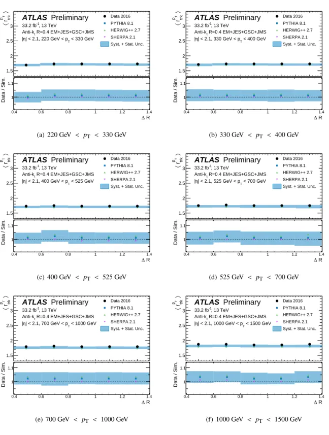
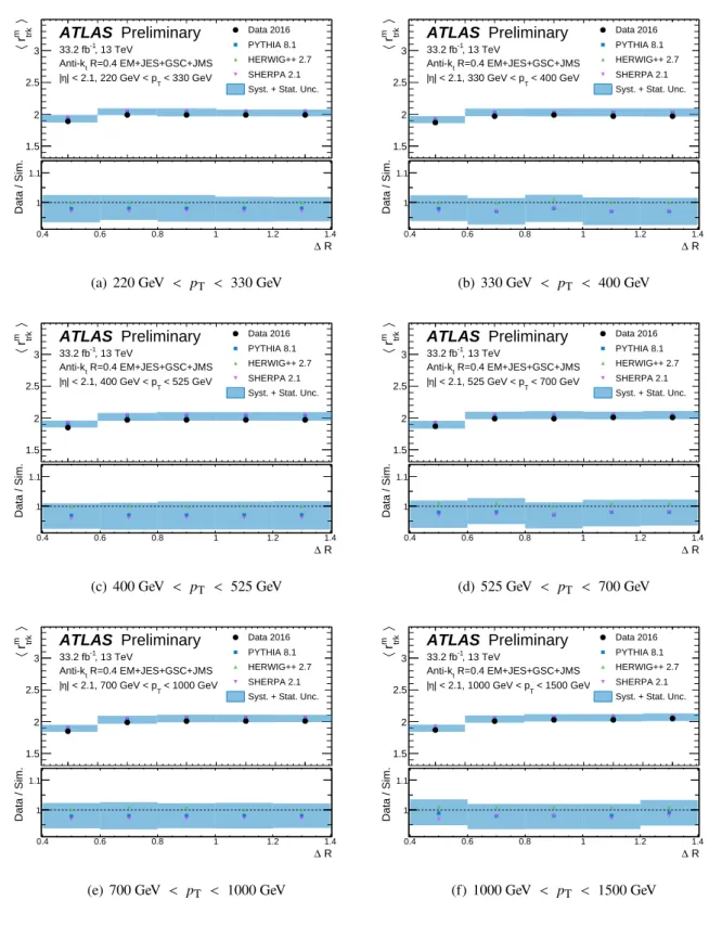
The median values of the probe jet calorimeter-to-track p

and mass responses in data and simulation are shown in figures 6-9, as functions of ∆R and f

. Excellent agreement between the median r

value in data and simulation is observed for both p

and mass responses, as a function of both close-by metrics, in each examined p

bin. The double-ratio of the median calorimeter-to-track response between data and simulation provides an estimate of the uncertainty on the calorimeter response. All ratios are found to be consistent with unity within uncertainties (propagated from the input distributions), and so no additional uncertainty is necessary to account for the effects of close-by radiation on jet modelling for input jets during the reclustering procedure.

It is possible that systematic mismodelling of jets due to close-by effects in simulation may manifest itself differently depending on the amount of close-by radiation which is present. In order to study this potential effect, triple ratios sensitive to these differences are defined by:

1. Constructing the r

ratio for a jet’s p

or mass.

2. Taking the ratio of the median r

value in environments with high and low amounts of close-by activity. High and low are defined respectively as above and below the median f

value from data within a given p

and m/p

bin.

3. Taking the ratio of the previous ratio between data and simulation.

This leads to the observables R

triple

and R

triple

:

R

triple

=

n

o

f_closeby^low

n

o

f_closeby^high

!

DATA

n

o

f^low closeby

n

o

f^high closeby

!

MC

, (6)

R

triple

=

n

o

f^low closeby

n

m^calo m^trk

o

f^high closeby

!

DATA

n

o

f_closeby^low

n

m^calo m^trk

o

f_closeby^high

!

MC

. (7)

These quantities should take a value near unity if close-by effects are consistently modelled as a function

of close-by activity. Many experimental systematic effects are also expected to cancel when building

0.5 1 1.5 2 2.5 3 3.5

Entries

100 200 300 400 500 600

103

×

ATLAS Preliminary

, 13 TeV 33.2 fb-1

< 330 GeV

| < 0.4, 220 GeV < pT

η

|

R=0.4 EM+JES+GSC+JMS Anti-kt

Data 2016 PYTHIA 8.1 HERWIG++ 2.7 SHERPA 2.1 Syst. + Stat. Unc.

pT

rtrk

0.5 1 1.5 2 2.5 3 3.5

Data / Sim.^0.5 1 1.5

(a)

0.5 1 1.5 2 2.5 3 3.5

Entries

50 100 150 200 250 300 350 400 450

103

×

ATLAS Preliminary

, 13 TeV 33.2 fb-1

< 330 GeV

| < 0.4, 220 GeV < pT

η

|

R=0.4 EM+JES+GSC+JMS Anti-kt

Data 2016 PYTHIA 8.1 HERWIG++ 2.7 SHERPA 2.1 Syst. + Stat. Unc.

m

rtrk

0.5 1 1.5 2 2.5 3 3.5

Data / Sim.^0.5 1 1.5

(b)

5 10 15 20 25 30 35 40 45

Entries

10 102

103

104

105

106

107

108

ATLAS Preliminary

, 13 TeV 33.2 fb-1

< 330 GeV

| < 0.4, 220 GeV < pT

η

|

R=0.4 EM+JES+GSC+JMS Anti-kt

Data 2016 PYTHIA 8.1 HERWIG++ 2.7 SHERPA 2.1 Syst. + Stat. Unc.

Closeby

f

5 10 15 20 25 30 35 40 45

Data / Sim.^0.5 1 1.5

(c)

0.4 0.5 0.6 0.7 0.8 0.9 1 1.1 1.2 1.3 1.4

Entries

100 200 300 400 500 600

103

×

ATLAS Preliminary

, 13 TeV 33.2 fb-1

< 330 GeV

| < 0.4, 220 GeV < pT

η

|

R=0.4 EM+JES+GSC+JMS Anti-kt

Data 2016 PYTHIA 8.1 HERWIG++ 2.7 SHERPA 2.1 Syst. + Stat. Unc.

∆ R

0.4 0.5 0.6 0.7 0.8 0.9 1 1.1 1.2 1.3 1.4

Data / Sim.^0.5 1 1.5

(d)

Figure 5: Representative distributions of the anti-k_t R =0.4 probe jet (a)r^pT

trk, (b)r^m

trk, (c) f_Closeby and (d)∆R, for jets withp_Tbetween 220 GeV and 330 GeV. The energy and mass of these jets have been calibrated, and they are built from topological clusters of calorimeter cells which have been calibrated at the electromagnetic scale. f_Closeby and∆Rrespectively quantify the amount of activity in the vicinity of a selected jet, and the smallest distance from a selected jet to another reconstructed jet. Each simulated sample is normalised to the integral of the data distribution.

Systematic uncertainties arising from the JES, JER and JMS are considered in these studies.

these ratios. Triple ratios of the probe jet p

and mass are respectively presented in figures 10 and 11, as a function of the probe jet m/p

. Agreement with unity is observed within the precision of the uncertainties, propagated from the input distributions to these ratios. Hence, the modelling of close-by effects as a function of the amount of activity is found to be consistently well-handled in Pythia, Herwig++

and Sherpa.

In all cases which have been studied within the context of jet reclustering, the modelling of the anti- k

R = 0 . 4 jets under study appears robust in the dense environments where significant close-by effects may be present. Pythia, Herwig++ and Sherpa each describe the trends of the median r

trk

and r

trk

values

in data well, as a function of the distance between reconstructed jets and the amount of radiation in the

vicinity of a jet. Based on these studies, it is concluded that it is not necessary to apply any additional

uncertainties to account for mis-modelling due to close-by effects in the context of jet reclustering.

0.5 0.6 0.7 0.8 0.9 1 1.1 1.2 1.3

〉Tp trk r〈

1.5 2 2.5 3

ATLAS Preliminary

, 13 TeV 33.2 fb-1

< 330 GeV

| < 2.1, 220 GeV < pT

η

|

R=0.4 EM+JES+GSC+JMS Anti-kt

Data 2016 PYTHIA 8.1 HERWIG++ 2.7 SHERPA 2.1 Syst. + Stat. Unc.

∆ R

0.4 0.6 0.8 1 1.2 1.4

Data / Sim. ¹ 1.1

(a) 220 GeV < p_T < 330 GeV

0.5 0.6 0.7 0.8 0.9 1 1.1 1.2 1.3

〉Tp trk r〈

1.5 2 2.5 3

ATLAS Preliminary

, 13 TeV 33.2 fb-1

< 400 GeV

| < 2.1, 330 GeV < pT

η

|

R=0.4 EM+JES+GSC+JMS Anti-kt

Data 2016 PYTHIA 8.1 HERWIG++ 2.7 SHERPA 2.1 Syst. + Stat. Unc.

∆ R

0.4 0.6 0.8 1 1.2 1.4

Data / Sim. ¹ 1.1

(b) 330 GeV < p_T < 400 GeV

0.5 0.6 0.7 0.8 0.9 1 1.1 1.2 1.3

〉Tp trk r〈

1.5 2 2.5 3

ATLAS Preliminary

, 13 TeV 33.2 fb-1

< 525 GeV

| < 2.1, 400 GeV < pT

η

|

R=0.4 EM+JES+GSC+JMS Anti-kt

Data 2016 PYTHIA 8.1 HERWIG++ 2.7 SHERPA 2.1 Syst. + Stat. Unc.

∆ R

0.4 0.6 0.8 1 1.2 1.4

Data / Sim. ¹ 1.1

(c) 400 GeV < p_T < 525 GeV

0.5 0.6 0.7 0.8 0.9 1 1.1 1.2 1.3

〉Tp trk r〈

1.5 2 2.5 3

ATLAS Preliminary

, 13 TeV 33.2 fb-1

< 700 GeV

| < 2.1, 525 GeV < pT

η

|

R=0.4 EM+JES+GSC+JMS Anti-kt

Data 2016 PYTHIA 8.1 HERWIG++ 2.7 SHERPA 2.1 Syst. + Stat. Unc.

∆ R

0.4 0.6 0.8 1 1.2 1.4

Data / Sim. ¹ 1.1

(d) 525 GeV < p_T < 700 GeV

0.5 0.6 0.7 0.8 0.9 1 1.1 1.2 1.3

〉Tp trk r〈

1.5 2 2.5 3

ATLAS Preliminary

, 13 TeV 33.2 fb-1

< 1000 GeV

| < 2.1, 700 GeV < pT

η

|

R=0.4 EM+JES+GSC+JMS Anti-kt

Data 2016 PYTHIA 8.1 HERWIG++ 2.7 SHERPA 2.1 Syst. + Stat. Unc.

∆ R

0.4 0.6 0.8 1 1.2 1.4

Data / Sim. ¹ 1.1

(e) 700 GeV < p_T < 1000 GeV

0.5 0.6 0.7 0.8 0.9 1 1.1 1.2 1.3

〉Tp trk r〈

1.5 2 2.5 3

ATLAS Preliminary

, 13 TeV 33.2 fb-1

< 1500 GeV

| < 2.1, 1000 GeV < pT

η

|

R=0.4 EM+JES+GSC+JMS Anti-kt

Data 2016 PYTHIA 8.1 HERWIG++ 2.7 SHERPA 2.1 Syst. + Stat. Unc.

∆ R

0.4 0.6 0.8 1 1.2 1.4

Data / Sim. ¹ 1.1

(f) 1000 GeV < p_T < 1500 GeV

Figure 6: The median value of ther^pT

trk response, for anti-k_tR=0.4 probe jets, as a function of∆R. The double-ratio ofr^pT

trkbetween data and simulation is shown in the lower panel. Statistical uncertainties and systematic uncertainties related to the JES, JER and JMS are shown as a blue band, propagated from the input distributions.

10 15 20 25 30 35 40 45

〉Tp trk r〈

1.5 2 2.5 3

ATLAS Preliminary

, 13 TeV 33.2 fb-1

< 330 GeV

| < 2.1, 220 GeV < pT

η

|

R=0.4 EM+JES+GSC+JMS Anti-kt

Data 2016 PYTHIA 8.1 HERWIG++ 2.7 SHERPA 2.1 Syst. + Stat. Unc.

Closeby

f

5 10 15 20 25 30 35 40 45

Data / Sim. ¹ 1.1

(a) 220 GeV < p_T < 330 GeV

10 15 20 25 30 35 40 45

〉Tp trk r〈

1.5 2 2.5 3

ATLAS Preliminary

, 13 TeV 33.2 fb-1

< 400 GeV

| < 2.1, 330 GeV < pT

η

|

R=0.4 EM+JES+GSC+JMS Anti-kt

Data 2016 PYTHIA 8.1 HERWIG++ 2.7 SHERPA 2.1 Syst. + Stat. Unc.

Closeby

f

5 10 15 20 25 30 35 40 45

Data / Sim. ¹ 1.1

(b) 330 GeV < p_T < 400 GeV

10 15 20 25 30 35 40 45

〉Tp trk r〈

1.5 2 2.5 3

ATLAS Preliminary

, 13 TeV 33.2 fb-1

< 525 GeV

| < 2.1, 400 GeV < pT

η

|

R=0.4 EM+JES+GSC+JMS Anti-kt

Data 2016 PYTHIA 8.1 HERWIG++ 2.7 SHERPA 2.1 Syst. + Stat. Unc.

Closeby

f

5 10 15 20 25 30 35 40 45

Data / Sim. ¹ 1.1

(c) 400 GeV < p_T < 525 GeV

10 15 20 25 30 35 40 45

〉Tp trk r〈

1.5 2 2.5 3

ATLAS Preliminary

, 13 TeV 33.2 fb-1

< 700 GeV

| < 2.1, 525 GeV < pT

η

|

R=0.4 EM+JES+GSC+JMS Anti-kt

Data 2016 PYTHIA 8.1 HERWIG++ 2.7 SHERPA 2.1 Syst. + Stat. Unc.

Closeby

f

5 10 15 20 25 30 35 40 45

Data / Sim. ¹ 1.1

(d) 525 GeV < p_T < 700 GeV

10 15 20 25 30 35 40 45

〉Tp trk r〈

1.5 2 2.5 3

ATLAS Preliminary

, 13 TeV 33.2 fb-1

< 1000 GeV

| < 2.1, 700 GeV < pT

η

|

R=0.4 EM+JES+GSC+JMS Anti-kt

Data 2016 PYTHIA 8.1 HERWIG++ 2.7 SHERPA 2.1 Syst. + Stat. Unc.

Closeby

f

5 10 15 20 25 30 35 40 45

Data / Sim. ¹ 1.1

(e) 700 GeV < p_T < 1000 GeV

10 15 20 25 30 35 40 45

〉Tp trk r〈

1.5 2 2.5 3

ATLAS Preliminary

, 13 TeV 33.2 fb-1

< 1500 GeV

| < 2.1, 1000 GeV < pT

η

|

R=0.4 EM+JES+GSC+JMS Anti-kt

Data 2016 PYTHIA 8.1 HERWIG++ 2.7 SHERPA 2.1 Syst. + Stat. Unc.

Closeby

f

5 10 15 20 25 30 35 40 45

Data / Sim. ¹ 1.1

(f) 1000 GeV < p_T < 1500 GeV

Figure 7: The median value of ther^pT

trk response, for anti-k_t R = 0.4 probe jets, as a function of f_Closeby. The double-ratio ofr^pT

trk between data and simulation is shown in the lower panel. Systematic and statistical uncertainties are shown as a blue band, propagated from the input distributions.