ATLAS-CONF-2014-003 17February2014
ATLAS NOTE
ATLAS-CONF-2014-003
February 17, 2014
Performance of shower deconstruction in ATLAS
The ATLAS Collaboration
Abstract
This note describes the performance of the shower deconstruction algorithm, a jet tag- ging algorithm, using proton-proton collisions at a centre of mass energy of
√s =
8 TeV.
Data recorded with the ATLAS detector corresponding to an integrated luminosity of 14.2 fb
−1are considered. Using small-radius jets to probe the substructure of a large-radius jet, shower deconstruction assigns a probability based on an approximate parton shower model, that the jet originated from a massive particle. In this note, the shower deconstruc- tion algorithm is investigated to identify jets produced from boosted, hadronically decaying top quarks. The performance is evaluated using events enriched in top-quark pairs in the lepton plus jets final state and a sample of dijet events. The distribution of the shower de- construction observable, the likelihood ratio
χSD, is compared between data and simulation and the expected performance of shower deconstruction is compared to that of other tagging algorithms.
c
Copyright 2014 CERN for the benefit of the ATLAS Collaboration.
Reproduction of this article or parts of it is allowed as specified in the CC-BY-3.0 license.
1 Introduction
1.1 Overview
Boosted heavy objects, such as vector bosons or top quarks with very high transverse momentum, p
T, are found in many new physics signals at the LHC. The decay products of a heavy particle produced with p
Tmuch greater than its mass are contained within a large-radius (large-R) jet. Many algorithms [1, 2]
have been proposed to identify and reconstruct boosted heavy particles by using the substructure of large-R jets. Shower deconstruction [3] (SD) is one such algorithm, combining information from the hard-scattering process, initial-state and final-state radiation, and colour flow.
In this note, the focus is on using SD as a top-tagger [4]. The input to SD is a collection of subjets clustered from the constituents of the large-R jet. These are used to calculate a likelihood ratio for the observed subjets to be produced by a hadronically decaying top quark compared to a multijet background process.
In this note, Section 1.2 describes the SD algorithm. Following a brief description of the ATLAS detector in Section 2, the data and Monte Carlo (MC) samples are described in Section 3. The perfor- mance of SD is examined in detail in Section 4 for events dominated by top quark pairs in the lepton plus jets final state, and briefly in Section 5 for dijet events. Finally, in Section 6, the expected top-tagging efficiency and background rejection of SD are compared to those obtained with other algorithms.
1.2 The shower deconstruction algorithm
The SD algorithm constructs a discriminant,
χSD, optimised to distinguish jets produced in decays of signal particles (S) from jets produced by background processes (B). In this note, the signal process used in the SD calculation is a hadronic top quark decay, and the background process is a jet originating from a single gluon. This background hypothesis could be improved by including also quark-initiated jets, but these are not implemented in the current version of the algorithm. The discriminant
χSDis derived considering the probabilities for parton showers from the signal and background process to produce the observed jet substructure.
The parton shower is a phenomenological approach to describe the emission of quarks and gluons in QCD bremsstrahlung radiation from incoming or outgoing quarks or gluons. In this approach, a 2
→N process with a complex final state is modelled starting from a simple 2
→2 process that approximately defines the directions and energies of the hardest partons. A succession of simple parton branchings are then added to build up the full event structure. This branching continues until the partons undergo hadro- nisation. The probability that a branching occurs is determined by Sudakov form factors and splitting functions [5] derived from the DGLAP equation [6, 7, 8]. A specific configuration containing N subjets with four-momenta
{p}
N = {p
1,p
2, . . . ,p
N}can be generated in many di
fferent ways in this approach, and each of these constitutes a possible shower history.
For a given shower history
{p, c
j}N, where j is the index of the shower history, each subjet with four momentum p
iis assigned to one of several categories c
ij. For signal, the categories are: the decay products of the top quark and their parton emissions; top parton radiation emission; and parton showers starting from initial-state radiation. Although it is usually considered negligible due to the short top- quark lifetime, parton radiation from the top quark itself may become significant for very highly boosted top quarks. It should be noted that here no additional information, such as b-tagging, is considered in the classification. For background, the categories are: final-state radiation; and initial-state radiation.
After assigning the subjets to categories, SD calculates the probability that a given shower history
was realised in a given event. A splitting probability is assigned to each branching, taking colour flow
into account. These probabilities are approximately the splitting probabilities that are used in parton-
shower event generators. Each propagator in the shower history corresponds to a Sudakov factor. By
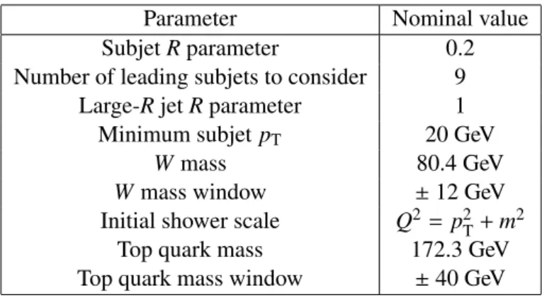
Table 1: List of shower deconstruction input parameters with their nominal values. For the initial shower scale, the p
Tand m are those of the large-R jet.
Parameter Nominal value
Subjet R parameter 0.2
Number of leading subjets to consider 9
Large-R jet R parameter 1
Minimum subjet p
T20 GeV
W mass 80.4 GeV
W mass window
±12 GeV
Initial shower scale Q
2 =p
2T+m
2Top quark mass 172.3 GeV
Top quark mass window
±40 GeV combining all of these propagators, shower histories are constructed [3, 4].
The shower histories are used to construct a likelihood ratio
χSD({p}
N) using the subjet four-vectors as inputs,
χSD
({ p}
N)
=P({ p}
N|S)P({p}
N|B) = Phistories
P({ p, c
j}N|S) Phistories
P(
{p, c
j}N|B) (1) where P(
{p}
N|S) is the probability of obtaining
{p}
Ngiven the signal hypothesis, and P(
{p}N|B) is the probability for obtaining
{p}Nfrom background jets arising from background processes. P({ p}
N|B) andP({ p}
N|S) are calculated as the sum of the probabilities for each shower history. The total probabil-ity depends on the number of shower histories considered, which is usually larger for the background hypothesis than for the signal hypothesis.
The signal and background have di
fferent colour structures and subjet kinematics because the sig- nal contains a massive electroweak-scale resonance decay with associated radiation, and the background comes only from splittings of energetic partons. These differences are reflected in the decay matrix element, splitting functions and the Sudakov factors, resulting in di
fferent values for P({p}
N|S) andP({ p}
N|B) when testing the same input. Thus, based on the kinematics of the subjets, the large-Rjet looks either more like a top jet or more like a QCD jet.
It is only possible to define
χSDwhen the subjets are kinematically compatible with a hadronic top quark decay. This leads to the following requirements: the jet has at least three subjets; two or more subjets must have a mass close to the W boson mass; and at least one more subjet can be added to obtain a total mass close to the top mass. Events failing these requirements have undefined
χSDand are labelled as
χSD(fail) in the subsequent sections and plots. Events satisfying these requirements are labelled as
χSD(pass). The mass windows and other parameters used in this study are listed in Table 1.
The computation time needed for the calculation of
χSDgrows exponentially with the subjet multiplicity, thus the input is restricted to the nine leading subjets of the leading large-R jet.
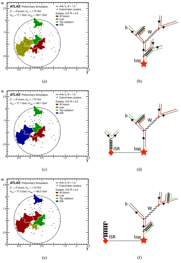
Figure 1 illustrates the SD algorithm for a simulated anti-k
t[9] large-R jet from Z
0→ttdecay for
m
Z0 =1.75 TeV. It has six Cambridge-Aachen (C/A) [10, 11] subjets, selected and reconstructed as
described in Section 4.3, from which more than 1500 (35000) possible shower histories for the signal
(background) hypothesis can be created. The three shower histories with the largest signal probabilities
are shown. Two features of SD are shown here. First, multiple interpretations of the substructure of a
jet are used. Here, two di
fferent combinations of subjets can be built with masses close to the W boson
mass. Second, all the input subjets are used by the algorithm; they are assigned to the top decay and
parton emissions from its decay products, to parton emission from the top or to initial-state radiation.
-1 -0.5 0 0.5 1 1.5 2 y2.5
φ
0 0.5 1 1.5 2
2.5 ATLAS Preliminary Simulation = 1.75 TeV mZ’
event, t
→t Z’
= 180.1 GeV mWb
= 77.7 GeV, mW
= 1.0
tR Anti-k
Calorimeter clusters = 0.2 Subjets, C/A R
boson W
jet b Top radiation ISR
(a) (b)
-1 -0.5 0 0.5 1 1.5 2 y2.5
φ
0 0.5 1 1.5 2
2.5 ATLAS Preliminary Simulation = 1.75 TeV mZ’
event, t
→t Z’
= 180.1 GeV mWb
= 77.7 GeV, mW
= 1.0
tR Anti-k
Calorimeter clusters = 0.2 Subjets, C/A R
boson W
jet b Top radiation ISR
(c) (d)
-1 -0.5 0 0.5 1 1.5 2 y2.5
φ
0 0.5 1 1.5 2
2.5 ATLAS Preliminary Simulation = 1.75 TeV mZ’
event, t
→t Z’
= 186.5 GeV mWb
= 77.3 GeV, mW
= 1.0
tR Anti-k
Calorimeter clusters = 0.2 Subjets, C/A R
boson W
jet b Top radiation ISR
(e) (f)
Figure 1: Illustration of the three (out of more than 1500) shower histories with the largest signal prob- abilities for a simulated large-R jet from a top quark produced in a Z
0→ttdecay with m
Z0 =1.75 TeV.
On the left panels are event displays showing the subjets used by the algorithm. Subjets of a particu- lar category have the same fill colour and their extent represents the subjet active catchment area [12].
Jet constituents are shown as black dots. On the right panels are the corresponding shower histories.
The hard scatter is indicated as the (red) star. Initial-state emissions are indicated by diamonds. Parton
emissions are indicated by filled circles. Coloured straight lines represent the colour flow.
2 The ATLAS detector
The ATLAS detector is described in detail in Ref. [13]. In this analysis, the trigger system, the calorime- ters and the muon system are of particular relevance.
The ATLAS inner detector, surrounded by a superconducting solenoid that provides a 2 T magnetic field, has full coverage in
φand covers the pseudorapidity range
|η|<2.5.
1It consists of a silicon pixel detector, a silicon strip detector and a transition radiation tracker.
The electromagnetic calorimetry (EM) is provided by the liquid argon (LAr) calorimeters that are split into three regions: the barrel (|η|
<1.475), the endcap (1.375
< |η| <3.2) and the forward (FCal:
3.1
< |η| <4.9) regions. The hadronic calorimeter is divided into four distinct regions: the barrel (|η|
<0.8), the extended barrel (0.8
<|η|<1.7), both of which are scintillator/steel sampling calorimeters, the hadronic endcap (1.5
< |η|<3.2), which has LAr
/Cu calorimeter modules, and the hadronic FCal (with the same
η-range as for the EM-FCal) which uses LAr/W modules. The total calorimeter coverage is
|η|<
4.9.
The muon spectrometer surrounds the calorimeters. It consists of multiple layers of trigger and track- ing chambers within an air-core superconducting toroidal magnetic field, which enables an independent, precise measurement of muon track momenta for
|η|<2.7.
ATLAS has a three-level trigger system [14]. A fast hardware-based level 1 trigger, is followed by two software-based triggers, the level 2 trigger which is located before the Event Builder and the Event Filter which perform increasingly fine-grained selection of events at lower rates.
3 Data and Monte Carlo samples
The analysis uses ATLAS data at a centre-of-mass energy of 8 TeV, corresponding to an integrated luminosity of 14.2 fb
−1collected up to September 2012.
The data are only used if they were recorded under stable beam conditions and all relevant subdetec- tors were at nominal operating conditions. For the study in Section 4, a logical OR of two single-muon triggers with p
Tthresholds of 24 GeV and 36 GeV over
|η|<2.4 and a logical OR of two single-electron triggers with p
Tthresholds of 24 GeV and 60 GeV over
|η|<2.47 are used. For the study in Section 5, a single-jet trigger with transverse energy threshold of 360 GeV is used.
The choice of MC generators is synchronized with that used in Refs. [15] and [16], to ensure that the results can be directly compared.
Standard Model tt production is modelled using the MC@NLO [17, 18] generator, with Herwig [19]
for parton showering and hadronisation and J
immy[20] for multiple-parton scattering (this combination is referred to as H
erwig/J
immysubsequently).
Additionally, for single-lepton triggered events, the background to tt events is produced using several generators. Single top quark production is modelled using MC@NLO showered by H
erwig/Jimmyin the s-channel [21] (or with an associated W boson [22]) and using A
cerMC [23] showered with P
ythia6 [24]
for the t-channel. Samples for production of W and Z bosons accompanied by jets are generated using A
lpgen[25], with up to five extra final-state partons at leading order without virtual corrections, and are showered by P
ythia6. The matching of the matrix element to the parton shower is done using the MLM method [26]. Massive-diboson production is modelled using H
erwig/J
immy. The multijet and W
+jets
1The ATLAS reference system is a Cartesian right-handed coordinate system, with the nominal collision point at the origin.
The anti-clockwise beam direction defines the positivez-axis, while the positivex-axis is defined as pointing from the collision point to the centre of the LHC ring and the positivey-axis points upwards. The azimuthal angleφis measured around the beam axis and the polar angleθis the angle measured with respect to thez-axis. The pseudorapidity is given byη=−ln tan(θ/2).
Transverse momentum is defined relative to the beam axis aspT= q
p2x+p2y=psinθ.
backgrounds are estimated fully or partly from the data, as described in Ref. [15], wherein more details of the data and MC samples can be found.
For the studies in Sections 5 and 6, MC dijet samples are modelled using Pythia8.
For the boosted top tagging study in Section 6, a sample of simulated high-p
Ttop quarks is used to determine the tagging e
fficiency. These are generated through a sample of Z
0with a mass, m
Z0, of 1.75 TeV decaying exclusively to tt in the semi-leptonic channel, modelled using Pythia8.
The samples were processed through the ATLAS detector simulation framework [27], which is based on Geant4 [28]. These simulations include a realistic modelling of the pile-up conditions observed in the data.
4 Performance of shower deconstruction using tt events
4.1 Event and object selections
This study uses events triggered by a single-lepton trigger that also contain a high-p
Tlarge-R jet re- constructed with the anti-k
talgorithm with R
=1.0, large missing transverse momentum, E
Tmiss, and a b-tagged jet. This gives a sample, dominated by tt production, that can be used to validate the perfor- mance of SD in events containing a boosted heavy particle.
Events must have a reconstructed primary vertex with at least five tracks with p
T ≥0.4 GeV. Also, extra requirements on E
Tmiss, the transverse mass
2, m
T, and the lepton kinematics are used to suppress multijet backgrounds:
•
Electron-triggered events are required to have:
–
exactly one trigger-associated reconstructed electron with E
T >25 GeV;
–
E
missT >30 GeV;
–
m
T >30 GeV.
•
Muon-triggered events are required to have:
–
exactly one trigger-associated reconstructed muon with p
T >25 GeV;
–
E
missT >20 GeV;
–
E
missT +m
T>60 GeV.
In addition, events must contain at least one b-tagged anti-k
tjet with R
=0.4 with no requirement on where this jet is in the event. This selection reduces contamination from W
+jets events. Finally, eventsare required to contain one trimmed [29] large-R jet with p
T ≥300 GeV and
|η| <1.2. In trimming, subjets are formed by applying a jet algorithm with smaller radius parameter, R
sub, and then soft subjets with less than a certain fraction, f
cut, of the original jet p
Tare removed. In this study, the trimming parameters used are f
cut=0.05 and R
sub=0.3.
Approximately 11500 events were obtained with a purity (defined as the number of expected tt events over the number of expected tt plus background events) of 70%. The multi-jet background, derived from data, accounts for only 3% of the expected events. Other backgrounds, such as single top, W
+jets, anddibosons, account for the remaining events, and are described by MC. In the following, we therefore label the total expectation as MC.
4.2 Systematic uncertainties
The sources of systematic uncertainties considered in this study can be split into two categories: uncer- tainties that a
ffect the modelling of the signal and background processes and uncertainties that a
ffect the reconstructed objects.
2The transverse mass is defined asmT = q
2pTEmissT (1−cos∆φ), wherepTis thepTof the charged lepton and∆φis the azimuthal angle between the charged lepton andEmissT .
For the first category, the dominant normalisation uncertainty comes from the t¯ t cross-section un- certainty of 11% [30]. The predicted central value and its total uncertainty is calculated consistently with Ref. [15]. They are evaluated at approximate NNLO in QCD [31] with Hathor 1.2 [30] using the MSTW2008 90% confidence-level NNLO PDF sets [32] and PDF+
αSuncertainties according to the MSTW prescription [33]. These uncertainties are then added in quadrature to the normalisation and factorisation scale uncertainty.
For the second category, the major contributions come from the jet energy scale (JES) for large-R jets and the b-tagging uncertainty. Uncertainties on the anti-k
tjets with R
=0.4, including the JES, jet reconstruction efficiency and jet energy resolution (JER), are also considered. Finally, uncertainties on the lepton isolation, trigger and reconstruction efficiency, as well as uncertainties on the missing energy reconstruction, are also evaluated and found to have a small impact.
Table 2 summarises the effect of the dominant systematic uncertainties on the total yield. A detailed description of the prescriptions followed to estimate the full list of systematic uncertainties can be found in Ref. [15].
Uncertainties on the acceptance from the scale and PDF choice in the MC, and uncertainties on the modelling of the underlying event are not considered, as they are much smaller than the sources listed in Table 2. Uncertainties due to the subjet energy scale, subjet energy resolution, and reconstruction e
fficiency are neglected in the study presented here, but their possible impact is briefly discussed in Sections 4.4 and 6.
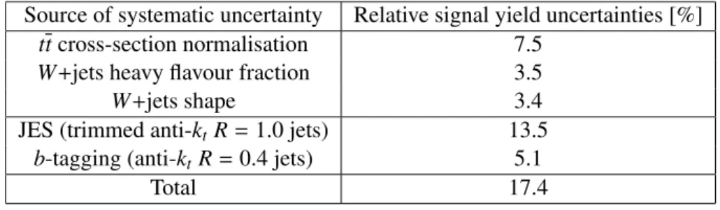
Table 2: Average impact of the dominant systematic uncertainties on the total predicted signal yield of large-R jets from boosted top-quark decays.
Source of systematic uncertainty Relative signal yield uncertainties [%]
tt cross-section normalisation 7.5
W
+jets heavy flavour fraction3.5
W
+jets shape3.4
JES (trimmed anti-k
tR
=1.0 jets) 13.5 b-tagging (anti-k
tR
=0.4 jets) 5.1
Total 17.4
4.3 Subjets and composite jets
The C/A jet-reconstruction algorithm is used as input to various jet substructure algorithms [2, 34, 16].
In this note C
/A jets with a radius parameter of 0.2 are used as input for SD.
As noted in Section 4.1, selected events contain a trimmed anti-k
tR
=1.0 jet with p
T ≥300 GeV.
The constituents of the original untrimmed anti-k
tR
=1.0 jet are clustered into C/A subjets with a radius parameter of 0.2. These jets are constructed in an independent step, which means, for example, that their area is not constrained by the area of the parent large-R jet (see Figure 1). Each subjet is calibrated in two subsequent steps [16]. First the contribution from pile-up is subtracted based on the median p
Tevent density multiplied by the subjet area. Next, energy and
η-dependent correction factors derivedfrom simulation are applied to bring the subjet to the hadronic scale.
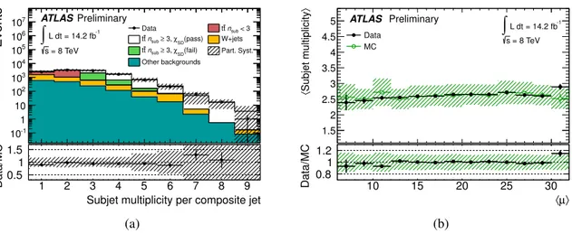
Subjets with p
T <20 GeV are discarded. After this cut is applied the mean subjet multiplicity (n
sub) shows little dependence on pile-up. Figure 2 shows the distribution of the subjet multiplicity.
It also shows the mean number of subjets for di
fferent pile-up conditions. The dominant systematic uncertainties arise from the trimmed anti-k
tR
=1.0 jet JES and from the t¯ t cross-section uncertainty.
The numerical value of the mean number of subjets is well predicted by the MC simulation and is not
Events
10-1
1 10 102
103
104
105
106
107 Data < 3
nsub t t (pass) χSD
≥ 3, nsub t
t W+jets
(fail) χSD
≥ 3, nsub t
t Part. Syst.
Other backgrounds
ATLASPreliminary
= 8 TeV s
L dt = 14.2 fb-1
∫
Subjet multiplicity per composite jet
1 2 3 4 5 6 7 8 9
Data/MC 0.5
1 1.5
(a)
t
mt
〉Subjet multiplicity〈
1.5 2 2.5 3 3.5 4 4.5
5 ATLAS Preliminary
= 8 TeV s
L dt = 14.2 fb-1
Data
∫
MC
〉 µ
〈
10 15 20 25 30
Data/MC 0.8
1 1.2
(b)
Figure 2: Number of C
/A R
=0.2 subjets with p
T ≥20 GeV for the leading composite jet (a) and mean subjet multiplicity versus
hµi(b), the mean number of collisions per bunch crossing. MC denotes the sum of all processes. The shaded area represents the total systematic uncertainty on the MC prediction, except systematics associated with the subjets. Data to MC prediction ratios are shown in the bottom panels.
strongly dependent on pile-up. The fraction of jets that arise from non-tt sources is higher at low subjet multiplicities.
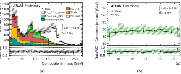
Figure 3 shows the mass distribution for composite jets defined by summing all of the subjet four- vectors considered by the SD algorithm (see Table 1). It also shows the mean mass for di
fferent pile-up conditions. The dominant systematic uncertainties arise from the trimmed anti-k
tR
=1.0 jet JES and from the t¯ t cross-section uncertainty. Composite jets with low masses are more likely to have less than the minimum requirement of three subjets, n
sub <3, and events with low-mass composite jets are more likely to fail the
χSDrequirements,
χSD(fail), listed in Table 1.
4.4 Shower deconstruction χ
SDobservable
A cut on the
χSDobservable can be used to enhance the fraction of top jets. Figure 4 shows the distri- bution of log(χ
SD). It also shows the mean log(χ
SD) for different pile-up conditions. Here, only events with
χSD(pass) are shown and therefore the fraction of the non-tt processes is smaller than in Figures 2 and 3. The fraction of events with
χSD(pass) is about 40% for tt and about 10% for non-tt processes.
The dominant systematic uncertainty arises from the trimmed anti-k
tR
=1.0 jet JES. The distribution of the mean of log(χ
SD) shows no significant dependence on pile-up. The distribution of the observable is reasonably well described by the MC prediction for this quite pure sample of jets from boosted-top-quark decay.
The observed data to MC di
fferences may be interpreted as being due to systematic uncertainties in the modelling of the underlying physics of signal or background, or of the detector. To study the potential impact on the performance from such uncertainties, a number of possible scenarios were investigated.
For example, a hypothetical 5% subjet energy scale uncertainty would a
ffect the shape and normalisation
of the log(χ
SD) distribution of both tt and background by an amount significantly larger than the observed
data versus MC differences in Figure 4.
Events / 10 GeV
0 200 400 600 800 1000 1200 1400 1600
Data ttnsub < 3
(pass) χSD
≥ 3, nsub t
t W+jets
(fail) χSD
≥ 3, nsub t
t Part. Syst.
Other backgrounds
ATLASPreliminary
L dt = 14.2 fb-1
∫
= 8 TeV s
Composite jet mass [GeV]
0 50 100 150 200 250
Data/MC 0.5
1 1.5
(a)
t
mt
[GeV]〉Composite jet mass〈
60 80 100 120 140
160 ATLAS Preliminary
= 8 TeV s
L dt = 14.2 fb-1
Data
∫
MC
〉 µ
〈
10 15 20 25 30
Data/MC 0.8
1 1.2
(b)
Figure 3: Jet mass for leading composite jet (a) and mean leading composite jet mass versus
hµi(b), the mean number of collisions per bunch crossing. MC denotes the sum of all processes. The shaded area represents the total systematic uncertainty on the MC prediction, except systematics associated with the subjets. Data to MC prediction ratios are shown in the bottom panels.
)SDχFraction of events / unit log(
0 0.05 0.1 0.15 0.2 0.25 0.3 0.35
Data W+jets
t
t Part. Syst.
Other backgrounds
ATLASPreliminary
L dt = 14.2 fb-1
∫
= 8 TeV s
(pass) χSD
SD) χ log(
-6 -4 -2 0 2 4 6 8
Data/MC 0.5
1 1.5
(a)
t
mt
〉) SDχlog(〈
2 3 4 5 6
7 ATLAS Preliminary
= 8 TeV s
L dt = 14.2 fb-1
Data
∫
MC
〉 µ
〈
10 15 20 25 30
Data/MC 0.8
1 1.2
(b)
Figure 4: Logarithm of the
χSDobservable for the leading composite jet (a) and mean log(χ
SD) versus
hµi(b), the mean number of collisions per bunch crossing. MC denotes the sum of all processes. The shaded
area represents the total systematic uncertainty on the MC prediction, except systematics associated with
the subjets. Data to MC prediction ratios are shown in the bottom panels.
Fraction of Events / 20 GeV 0.02 0.04 0.06 0.08 0.1 0.12 0.14
0.16 ATLAS Preliminary
L dt = 14.2 fb-1
∫
= 8 TeV s
(pass) χSD
Data Pythia Dijets
[GeV]
Composite jet pT
550 600 650 700 750 800 850 900 950 1000
Data/MC 0.5
1 1.5
(a)
) SDχFraction of events / unit log(
0 0.02 0.04 0.06 0.08 0.1 0.12 0.14 0.16 0.18
0.2 ATLAS Preliminary
L dt = 14.2 fb-1
∫
= 8 TeV s
(pass) χSD
Data Pythia Dijets
SD) χ log(
-10 -8 -6 -4 -2 0 2 4
Data/MC 0.5
1 1.5
(b)
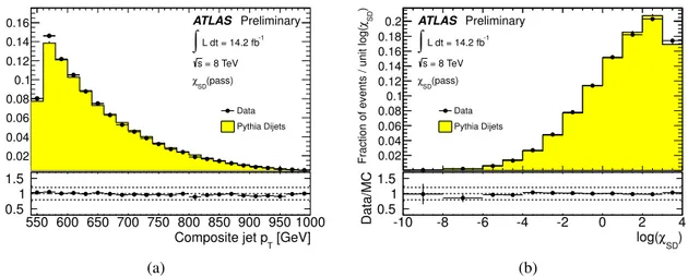
Figure 5: Distribution of the composite jet p
T(a) and logarithm of the
χSDobservable (b) for the leading composite jet in dijet events. Data to MC prediction ratios are shown in the bottom panels.
5 Data to Monte Carlo comparison using dijet events
This study uses events triggered by a single-jet trigger. Systematic uncertainties are not taken into ac- count in this context.
Dijet candidate events are required to have at least two trimmed anti-k
tR
=1.0 jets with p
T≥300 GeV and
|η|<1.2. The two leading jets are required to have
∆φ≥2.6. The leading large-R jet must have p
T≥550 GeV, to be consistent with the kinematic requirements used in the top-tagging comparison in Section 6. The subjets are constructed in the same way as for the tt studies (see Section 4.3).
Figure 5 shows a data to MC shape comparison of the distribution of composite jet p
Tin the range 550-1000 GeV for events with
χSD(pass). The predicted MC shape agrees within 10% with the data across the full spectrum. A data to MC comparison of the distribution of log(χ
SD) is also shown. Also here, the largest statistically significant data to MC di
fference is less than 10%. Data is not shown for log(χ
SD)
>4 as this corresponds to the region where signal could be expected from jets produced in the decays of heavy particles, as will be described in Section 6.
6 Expected performance of shower deconstruction for Z
0→tt decays
In this section, a study of top-tagging efficiency and background rejection with SD is performed using MC samples. As noted in Section 3, high-p
Ttop quarks are obtained using a sample of Z
0→ttdecays with m
Z0 =1.75 TeV and background light quark and gluon jets are obtained using the dijet sample described in Section 5. The input samples and selection criteria used are identical to those used in Ref. [16] to facilitate a direct comparison between di
fferent algorithms. Here the leading large-R jet is required to have p
T≥550 GeV and
|η|<1.2.
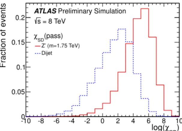
Figure 6 shows the shape of log(χ
SD) for signal and background. For the selected jets, log(χ
SD) has an average value of approximately five for top-jets and two for multijets. This was shown in Figure 4a for top-jets with a lower p
T-threshold of the large-R jet and in Figure 5b for background jets in the same large-R jet kinematic region. This figure illustrates how a cut on log(χ
SD) will help to discriminate between signal and background.
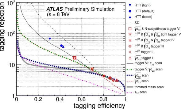
By varying the cut on log(χ
SD), one obtains the background rejection (defined as the reciprocal of
the efficiency) versus signal efficiency curve for SD. This is shown in Figure 7, where SD is compared
SD) log(χ
-10 -8 -6 -4 -2 0 2 4 6 8 10
Fraction of events
0 0.05 0.1 0.15 0.2
Z’ (m=1.75 TeV) Dijet
ATLASPreliminary Simulation = 8 TeV
s (pass) χSD
Figure 6: Logarithm of the
χSDobservable for signal Z
0 →tt and background multijet simulated samples (shown in Figure 5b) for events satisfying the minimum requirements of the SD algorithm.
to other tagging techniques from Ref. [16]. The best background rejection over a wide range of signal e
fficiencies is obtained with SD, but it should be noted that none of the expected performances shown here account for possible systematic uncertainties. The maximum signal efficiency and minimum background rejection are given by the fraction of events satisfying the minimum requirements of the SD algorithm.
For the signal studied here, this fraction is about 70%
3, for background, it is approximately 12%. These values are consistent with those of the tight tagger V shown in Figure 7. This tagger uses a lower cut on the trimmed large-R jet mass of 100 GeV, and lower cuts of 40 and 10 GeV on the large-R jet first and second k
tsplitting scales respectively.
Propagating the hypothetical 5% subjet energy scale uncertainty, discussed in Section 4.4, through to the e
fficiency and background rejection, results in a maximum signal e
fficiency drop of about 2%, and a background rejection degradation of up to 30%.
7 Summary
An application of the shower deconstruction algorithm as a top-quark-tagger is implemented using the ATLAS detector. The performance of this algorithm has been examined in detail for data and MC samples of events predominantly arising from top-quark pair production observed in the lepton plus jets final state. The data were compared to simulation for three key observables, the subjet multiplicity, the composite jet mass defined by the mass of the sum all of the subjet four-vectors considered by the SD algorithm, and the log(χ
SD) observable. Satisfactory agreement was found between data and simulation as well as stable performance as a function of the pile-up conditions.
The expected performance of the SD algorithm and of other top-tagging and substructure techniques has been estimated using samples of simulated high- p
Ttop quarks from Z
0→ttdecays with m
Z0 =1.75 TeV as the signal and dijets as the background. For this scenario, the SD algorithm shows the best light quark and gluon jet background rejection over a wide range of top-jet signal efficiencies, when systematic uncertainties are not considered.
3This fraction is higher than in thettsample described in Section 4.4 because of the larger average boost of the top-quarks.
tagging efficiency
0 0.2 0.4 0.6 0.8 1
tagging rejection
1 10 10
210
3 HTT (tight)HTT (default) HTT (loose) SD
& N-subjettiness tagger VI d12
tight tagger V d23
&
d12
&
mjet
tagger IV d23
&
d12
&
mjet
tagger III d12
&
mjet
tagger II mjet
tagger I d12
scan τ32
tagger VI:
scan d23
tagger V:
scan d12
scan d23
trimmed mass scan scan
τ32
ATLAS Preliminary Simulation = 8 TeV
s
Figure 7: Comparison of expected top jet tagging efficiency and light quark/gluon jet rejection. All substructure taggers and scans use trimmed anti-k
tR
=1.0 jets, except the HEPTopTagger (HTT) that uses C
/A R
=1.2. The same Z
0→tt, m
Z0 =1.75 TeV signal samples and multijet background samples and selection are used for all taggers. Systematic uncertainties are not considered for any of the algorithms.
References
[1] A. Altheimer et al., Jet Substructure at the Tevatron and LHC: New results, new tools, new benchmarks, J. Phys.
G39(2012) 063001, arXiv:1201.0008 [hep-ph].
[2] ATLAS Collaboration, Performance of jet substructure techniques for large-R jets in proton-proton collisions at
√s
=7 TeV using the ATLAS detector, JHEP
1309(2013) 076, arXiv:1306.4945 [hep-ex].
[3] D. E. Soper and M. Spannowsky, Finding physics signals with shower deconstruction, Phys. Rev.
D84