The ATLAS Collaboration

ATLAS-CONF-2017-068 25September2017

ATLAS CONF Note

CONF-HION-2017-068

September 17, 2017

Measurement of long-range azimuthal correlations in Z -boson tagged pp collisions at √

s = 8 TeV

The ATLAS Collaboration

September 17, 2017

This analysis is the first to study long-range hadron correlations inppcollisions with a con- straint on collision geometry. The constraint is implemented by requiring events in which aZboson is produced, which is a high-Q²hard scattering process related to the impact pa- rameter of theppcollision. The analysis is performed using 19.4 fb⁻¹ of √

s = 8 TeV pp data obtained by the ATLAS detector during the physics Run-1 of the LHC. The sample con- tains approximately 6.2×10⁶ selectedZ-boson candidate events. The correlations between the charged-particle pairs in relative azimuthal angle over the transverse momentum range from 0.5 GeV to 5 GeV are studied as a function of the charged particle multiplicity of the event. The average number of interactions per bunch crossing in the data sample is about 20, therefore the number of charged particle tracks and the correlation functions are corrected to account for the significant pileup contribution present in the events. The correlations between particle pairs is quantified by the second Fourier coefficient,v_2,2, which in turn is used to ob- tain the single-particle anisotropy coefficientv₂. Thev₂coefficient in theZ-tagged events is found to be independent of multiplicity as previously observed in inclusive ppevents, and its magnitude is found to be 8±6% larger than that in inclusiveppevents.

c

2017 CERN for the benefit of the ATLAS Collaboration.

1 Introduction

Measurements of two particle correlations (2PC) in relative¹azimuthal angle∆φ =φ^a−φ^b and pseudo- rapidity separation∆η = η^a−η^b in proton–proton (pp) collisions show the presence of correlations in

∆φ at large η separation [1–3]. Recent studies by the ATLAS Collaboration demonstrated that these long-range correlations are consistent with the presence of a cos (nφ) modulation of the single particle azimuthal angle distributions [2, 3], similar to that seen in Pb+Pb and p+Pb collisions [1, 4–6]. The modulation of the single-particle azimuthal angle distributions is typically characterized using a set of Fourier coefficientsvn, that describe the relative amplitudes of the sinusoidal components of the single- particle distributions:

dN dφ ∝







1+2

∞

X

n=1

vncos

n(φ−Φn)







, (1)

where thevnandΦndenote the magnitude and orientation of the single-particle anisotropies.

In nuclei-nuclei (A+A) and proton-nuclei (p+A) collisions, the vn result from anisotropies of the ini- tial collision geometry which are subsequently transferred to the azimuthal distributions of the produced particles by the collective evolution of the medium. This transfer of the spatial anisotropies in the initial collision geometry to anisotropies in the final particle distributions, is well described by relativistic hydro- dynamics [7–9]. The ATLAS measurements in Ref. [3] show that the p_Tdependence of the second-order harmonic,v2, in ppcollisions, is similar to thev2observed in the other systems. Additionally, thev2inpp collisions shows no dependence on the center-of-mass collision energy, √

s, from 2.76 TeV to 13 TeV, similar to what is observed in p+A and A+A collisions [10–12]. These striking similarities between the p_T and √

sdependence of the v2 in ppcollisions to thev2in A+A andp+A collisions indicate the possibility of collective behavior developing inppcollisions, though alternate models that qualitatively reproduce the features observed in thepp2PC exist [13–18].

One feature in which the pp v₂ differs from the v₂ in p+A and A+A collisions, is that the pp v₂ is independent, within uncertainties, of the event multiplicity, while the p+A and, especially, the A+A v₂ exhibit considerable dependence on the event multiplicity. This dependence is due to a correlation between the collision geometry and collision impact parameter (b). In collisions with smallbthe second order eccentricity (₂) of the initial geometry is small resulting in a relatively reducedv₂. Interactions atb comparable to the size of a nucleus result in an overlap region that becomes increasingly elliptic, with₂ increasing withb. This, in turn, generates larger v₂. Thus, the strong correlation between the v₂ and multiplicity is in fact the result of the dependence of the collision geometry on the b. There have been multiple theoretical studies in A+A andp+A collisions which reproduce thebdependence of thevn quite well. However, there are very few such calculations for ppcollisions. A recent study that models the proton substructure and fluctuations in the multiplicity of the final particles, showed that the eccentricities₂and₃of the initial entropy-density distributions inppcollisions have no correlation with the final particle multiplicity [19].

In this note the long-range correlations of charged particles are measured in ppinteractions that have a Zboson produced in the collision. The presence of aZboson selects an event in which there was a hard scattering (with Q² ≈ 80 GeV²), which may lower the partonic b. An assumption driven by the A+A collisions is that if the ppv₂is related to the eccentricity of the collision geometry, then events ‘tagged’

by aZboson having a smallerbmight also have smallerv₂than that measured in inclusive events.

1 The labelsaandbdenote the two particles in the pair.

The data used in previous ATLAS pp-ridge studies [2, 3], were recorded under conditions of relatively low instantaneous luminosity, for which the number of collisions per bunch crossing (µ), was µ . 1.

However theZ-boson dataset used in the present analysis comes from significantly higher luminosity conditions, with the typicalµof about 20. This large luminosity poses significant complications to the correlation analysis, as it is not possible to separate reconstructed tracks from simultaneous interactions (pileup) from the tracks associated with the interaction producing theZboson. To solve the problem of pileup tracks a new procedure is developed that removes the contribution of such tracks on a statistical basis.

The note is organized as follows. Section2 gives a brief overview of the ATLAS detector subsystems used in this analysis. Section3 describes the dataset, triggers and the offline selection criteria used to select events and reconstruct charged-particle tracks used in the analysis. Section4gives a brief overview of the two-particle correlation method and how it is used to obtain thev₂. Section5details the corrections applied for analyzing data in presence of the background coming from the pileup. The correlations are calculated between hadron-pairs as in Refs. [2,3]. The systematic uncertainties are detailed in Section7 and the results are presented and discussed in Section8. Section 9gives a summary of the main results and observations.

2 ATLAS detector

The ATLAS detector [20] at the LHC covers nearly the entire solid angle around the collision point. It consists of an inner tracking detector surrounded by a thin superconducting solenoid, electromagnetic and hadronic calorimeters, and a muon spectrometer incorporating three large superconducting toroid magnets. The inner-detector system (ID) is immersed in a 2 T axial magnetic field and provides charged particle tracking in the range|η|<2.5.²

The high-granularity silicon pixel detector covers the vertex region and typically provides three mea- surements per track, the first hit being normally in the innermost layer. It is followed by the silicon microstrip tracker which usually provides four two-dimensional measurement points per track. These silicon detectors are complemented by the transition radiation tracker, which enables radially extended track reconstruction up to|η|= 2.0. The transition radiation tracker also provides electron identification information based on the fraction of hits (typically 30 in total) above a higher energy deposit threshold corresponding to transition radiation.

The calorimeter system covers the pseudorapidity range|η| < 4.9. Within the region|η| < 3.2, electro- magnetic calorimetry is provided by barrel and endcap high-granularity lead/liquid-argon (LAr) electro- magnetic calorimeters, with an additional thin LAr presampler covering|η| < 1.8, to correct for energy loss in material upstream of the calorimeters. Hadronic calorimetry is provided by the steel/scintillating- tile calorimeter, segmented into three barrel structures within |η| < 1.7, and two copper/LAr hadronic endcap calorimeters. The solid angle coverage is completed with forward copper/LAr and tungsten/LAr calorimeter modules optimised for electromagnetic and hadronic measurements respectively.

2ATLAS uses a right-handed coordinate system with its origin at the nominal interaction point (IP) in the centre of the detector and thez-axis along the beam pipe. The x-axis points from the IP to the centre of the LHC ring, and they-axis points upwards. Cylindrical coordinates (r, φ) are used in the transverse plane,φbeing the azimuthal angle around thez-axis. The pseudorapidity is defined in terms of the polar angleθasη=−ln tan(θ/2).

The muon spectrometer (MS) comprises separate trigger and high-precision tracking chambers measuring the deflection of muons in a magnetic field generated by superconducting air-core toroids. The precision chamber system covers the region |η| < 2.7 with three layers of monitored drift tubes, complemented by cathode strip chambers in the forward region, where the background is highest. The muon trigger system covers the range|η|<2.4 with resistive plate chambers in the barrel, and thin gap chambers in the endcap regions. A three-level trigger system is used to select interesting events [21]. The Level-1 trigger is implemented in hardware and uses a subset of detector information to reduce the event rate to a design value of at most 75 kHz. This is followed by two software-based trigger levels which together reduce the event rate to about 200 Hz.

3 Datasets, event and track selection

The analysis is based on ppcollisions at √

s = 8 TeV. The data sample used, corresponding to a total integrated luminosity of 19.4 fb⁻¹, was recorded between April and December 2012. The uncertainty in the integrated luminosity is±2%. All data used in the analysis come from data-taking periods in which the beam and detector operations were stable.

Z-boson events are reconstructed via the di-muon channel. Events are first selected based on either a di-muon or high-p_T single muon trigger. Muons are reconstructed as combined tracks spanning both the ID and the MS [22]. Muon candidates withp_T >20 GeV and|η|<2.4 are selected for pairing. Events in which there are exactly two muon candidates with opposite charge and invariant mass between 80 GeV and 100 GeV are consideredZ-boson candidate events. For studies of the background due to multiple interactions per bunch crossing,zero biasdata was used. This data was collected at the same time as the (di-)muon triggered data, but recorded based on a trigger which is effectively random with respect topp interactions.

In theZ-boson candidate events (‘Z-tagged’ events), charged particle tracks reconstructed in the ID are used for the two-particle correlation analysis. The tracks selected for this analysis are required to pass the standard set of quality requirements on the number of used and missing hits in the detector layers according to the track reconstruction model [23]. To suppress the number of tracks coming from the secondary particles, the distance of the closest approach of the track to the event vertex in the transverse plane is restricted to be less than 1.5 mm. In addition, the longitudinal impact parameter of the track relative to the vertex is required to be less than 0.75 mm. As in previous ATLAS analyses of long- range correlations in p+Pb and pp collisions, the event activity is quantified by the total number of reconstructed charged-particle tracks passing quality requirements, and with p_T>0.4 GeV [2,3,6, 24].

The track multiplicity is also corrected to account for pileup (see Section5). The muon tracks that are associated with theZ-boson decay are not considered in the analysis.

4 Two-particle correlations

The study of two-particle correlations in this note follows previous ATLAS measurements inppcollisions [2,3] , with the additional complication of handling the pileup, which is discussed later in Section5. The two-particle correlations are measured as a function of the relative azimuthal angle ∆φ ≡ φ^a −φ^b for particles separated by|∆η|>2. This gap is used to study the long-range component of the correlations [2,

3]. The labels a and b denote the two particles in the pair, and are conventionally referred to as the

“reference” and “associated” particles, respectively. The correlation function is defined as:

C(∆φ)= S(∆φ)

B(∆φ) , (2)

where S represents the pair distribution constructed using all particle pairs that can be formed from tracks that are associated with the event containing theZ-boson candidate and pass the required selection criteria. TheS distribution contains both the physical correlations between particle pairs and correlations arising from detector acceptance effects. The pair-acceptance distributionB(∆φ), is similarly constructed by choosing the two particles in the pair from different events. The B distribution does not contain physical correlations, but has detector acceptance effects identical to those inS. In taking the ratio,S/B in Eq. (2), the detector acceptance effects cancel, and the resultingC(∆φ) contains physical correlations only. To correctS(∆φ) andB(∆φ) for the individualφ-averaged inefficiencies of particlesaandb, the pairs are weighted by the inverse product of their tracking efficiencies 1/(ab). Statistical uncertainties are calculated forC(∆φ) using standard uncertainty propagation procedures assuming no correlation between S andB, and with the statistical variance ofS andBin each∆φbin taken to beP1/(ab)², where the sum runs over all of the pairs included in the bin. The two-particle correlations are used only to study the shape of the correlations in ∆φ, and their overall normalization does not matter. In this note, the normalization ofC(∆φ) is chosen such that the∆φ-averaged value ofC(∆φ) is unity.

The strength of the long-range correlation can be quantified by extracting Fourier moments of the 2PC.

The Fourier coefficients of the 2PC are designated asvn,nand defined by:

C(∆φ)=C₀(1+2X

n

v_n,ncos(n∆φ)). (3)

Thev_n,n are directly related to the single-particle anisotropiesvn described in Eq. (1). For reference and associated particles with p_T = p^a_T and p^b_T respectively, thevn,n(p^a_T,p^b_T) is the product of thevn(p^a_T) and vn(p^b_T) [25], i.e.:

vn,n(p^a_T,p^b_T)=vn(p^a_T)vn(p^b_T). (4) Thus, thevn(p^a_T) can be obtained as:

vn(p^a_T)= v_n,n(p^a_T,p^b_T)

vn(p^b_T) = v_n,n(p^a_T,p^b_T) qv_n,n(p^b_T,p^b_T)

, (5)

wherevn,n(p^b_T,p^b_T) is the Fourier coefficient of the 2PC produced when taking both reference and asso- ciated particle to be from the same p_T range. This technique has been used extensively in heavy-ion collisions to obtain the flow harmonics [25]. However, in ppcollisions significant contribution to the 2PC arises from back-to-back dijets (which can correlate particles at large|∆η|). These correlations must be removed before Eq. (4) or Eq. (5) can be used. In order to estimate and remove the contribution of such back-to-back dijets and other correlations which correlate only a subset of the total particles in the event, a template fitting method was developed and used in two recent ATLAS measurements [2,3]. The template fitting procedure assumes that:

1. The jet-correlation has identical shape in∆φin low multiplicity and in higher multiplicity events.

Change is in the relative contribution of the dijets to the 2PC.

2. At low multiplicity most of the structure of the 2PC arises from back-to-back dijets, i.e. the shape of the dijet correlation can be obtained from low multiplicity events.

With the above assumptions, the correlation in higher multiplicity eventsC(∆φ), is then described by a template fit, C^templ(∆φ) consisting of two components: 1) the correlation that accounts for the dijet contribution,C^periph(∆φ), measured in low multiplicity and scaled by a factor F, and 2) genuine long- range harmonic modulation,C^ridge(∆φ):

C^templ(∆φ)=FC^periph(∆φ)+G







1+2X

n=2

v_n,ncos(n∆φ)







 (6)

≡FC^periph(∆φ)+C^ridge(∆φ).

where, the coefficientFand thevn,nare fit parameters adjusted to reproduce theC(∆φ). The coefficientG is not a free parameter, but is fixed by the requirement that the integrals of theC^templ(∆φ) andC(∆φ) over the full∆φrange be equal.

This analysis uses the 20–30 multiplicity interval as the peripheral reference. This choice is different from the analysis in Refs. [2,3] where the 0–20 interval was used. This change is due to a low number of events with less than 20 tracks in theZ-tagged sample that affects the statistical precision of the periph- eral reference. The systematic uncertainty associated with the choice of higher multiplicity peripheral reference is evaluated by comparingv₂results when using other peripheral intervals, including 0–20.

5 Pileup subtraction

5.1 Event Categories

The analysis presented in this note is based on the √

s = 8 TeV ppevent sample obtained in nominal LHC running conditions. Over the entire sample of 19.4 fb⁻¹ the average number of interaction per bunch crossing isµ≈20, the average number of reconstructed vertices [26] found in the data is approx- imately 11.5, and the average number of tracks per event satisfying the above mentioned conditions is approximately 180. Most of these tracks are coming from the pileup interactions, i.e. the inclusive pp interactions that occur in the same bunch crossing as the event producing theZ boson that fired the trig- ger. The ATLAS ID tracking system allows rejecting most of such tracks by requiring that the distance from the point of the track intersection with the beam axis in longitudinal direction (z₀) falls in a narrow windowωfrom theZ-boson interaction vertex (z_vtx),

ω=(z₀−z_vtx)sin(θ) (7)

whereθis the polar angle of the track and the value|ω|<0.75 mm is used in the analysis that reduces the number of tracks by factor of 6.

Tracks passing the selection criteria listed above still contain a significant contribution of the tracks orig- inating from pileup interactions. This residual pileup contribution is corrected for statistically using the procedure described below. All tracks in a single event that are selected for the analysis are considered to comprise theDirectevent. It is the sum of 2 events, theSignalevent formed by tracks that are coming

from the same interaction as theZboson, and theBackgroundevent formed by all other tracks. Tracks in the Background event, may come from one or more pileup interactions.

Presence of the Background event in the Direct affects both the number of measured tracks (n_trk) and the two particle correlations. To measure characteristics of the Signal events, the contribution of Background events needs to be subtracted, for which a sample of events equivalent to the Background events is con- structed. This is done using a random selection procedure, described further in the text, and the sample of events obtained by the procedure is denoted as theMixedevent sample. The numbers of tracks in the corresponding event categories are denoted asn^direct_trk ,n^signal_trk , andn^mixed_trk .

5.2 Mixed event sample

The random selection procedure is an extension of a technique used in a previous ATLAS analysis [27]. It constructs an event that is similar to the Direct event, but contains no Signal component in it. It is done by selecting tracks according to Eq.7in one event with respect to thez_vtxmeasured in another Direct event.

Both events are required to haveµwithin the same integer count and be taken during the same beam fill of the LHC. These requirements are to ensure that the detector conditions and thez_vtxdistribution in the 2 events are close to each other so that the Mixed event is constructed in the same instantaneous luminosity conditionµas the Direct event. To account for differences in thez_vtx distribution in different LHC fills that occur over the duration of the √

s =8 TeV ppdata taking, the analysis uses reduced value ofµand z_vtxthat are:

( ¯µ,z¯_vtx)= µ

√2πRMS(z_vtx),z_vtx− hz_vtxi RMS(zvtx)

!

, (8)

wherehz_vtxiand RMS(z_vtx) are the mean and width of thez_vtxdistribution averaged over the data of one LHC fill, and √

2πis the normalization coefficient of the Gaussian shape. The reduced value of ¯µ is measured in units of mm⁻¹and typical value of RMS(zvtx) in the data sample is about 47 mm.

Event samples used by the random selection procedure can be obtained with a random trigger or with the same trigger as the Direct event sample. In the latter case, an additional condition must be used that requires the distance between thez_vtx positions in 2 events to be |∆z_vtx| > 15 mm. This is to ensure that the tracks from the interaction that fires the trigger and have particle counts and kinematics different from the inclusive (pileup) interactions do not contribute to the Mixed event that is reproducing only the Background component. Mixed events constructed with both samples yield identical results, therefore the analysis uses the same trigger event sample as the Direct events that automatically insures identical data taking conditions in Direct and Mixed events. The procedure is validated using the Monte Carlo simulation sample and shows that the distributions found in Mixed event are equivalent to those in the Background events. To suppress undesired statistical fluctuations in the Mixed event sample the random selection procedure is performed 20 times for each Direct event.

Figure1shows the average track density in Direct and Mixed events for different values of ¯z_vtx and ¯µ.

The panels show three intervals of ¯z_vtx position and different marker colors denote different ¯µintervals.

Full markers are the results measured in Direct events and open markers in Mixed events. In all curves belonging to Direct events the Signal tracks form the peak at origin and the Background tracks form the substrates outside and under the peak. Solid lines are the fits to the substrates made outside the peak regions and interpolated under the peaks. There is good agreement between the results of the fits and the results of Mixed events in the region under the peak. The Mixed points are slightly lower than the

[mm]

ω

-4 -2 0 2 4

] -1 [mmz/d trknd

1 2 3 4 5 6

≤-1.6 zvtx

≤ a) -2.4

Preliminary ATLAS

=8TeV, 19.4fb-1

s , pp

[mm]

ω

-4 -2 0 2 4

≤0.4 zvtx

≤ b) -0.4

[mm]

ω

-4 -2 0 2 4

≤1.6 zvtx

≤

c) 0.8 0.26≤µ≤0.27

≤0.23

≤µ 0.22

≤0.19 µ

≤ 0.18

≤0.15

≤µ 0.14

≤0.11 µ

≤ 0.10

≤0.07 µ

≤ 0.06

Figure 1: Number of tracks per mm as a function ofωdefined by Eq. (7). The three panels show results in different intervals of the reduced vertex ¯zvtx position and different marker colors correspond to several intervals of reduced µ. Full markers show the Direct event and open markers show Mixed events. Solid lines are parabolic fits to Direct¯ events in the region|ω|>4 mm and vertical dash lines show the acceptance window|ω|<0.75 mm.

curves, consistent with the effect of secondary particles contributing to the substrate outside the peak region elevating the fitting curve above the real Background values. At the values of|ω| > 2.45 mm, Mixed curves in all ( ¯µ,¯z_vtx) intervals depart from the Direct ones. This is due to the contribution of collisions that fired the trigger. Then_trkin them is larger than in the pileup interaction causing the excess.

However, due to the requirement that|∆z_vtx|between the Direct event and the event used by the random selection procedure must be greater than 15 mm, no tracks from triggered collisions can affect the region of|ω|<0.75 mm. Tracks from such interactions with the smallest possible angle in the acceptance of the ID system,θ=0.164 corresponding to|η|=2.5, only appear at the distance|∆z_vtx|sin(θ)=2.45 mm. This effect does not appear when the random selection procedure uses zero bias sample, where the requirement of|∆z_vtx|>15 mm is not applied.

Based on the agreement demonstrated by Fig.1, and on the Monte Carlo (MC) simulation studies, this analysis uses the assumption that then_trk distributions (number of counts, kinematical variables and two particle correlations) in the Mixed events are equivalent to the distributions of the Background events:

Direct=Signal+Background,

Mixed≡Background. (9)

5.3 Background estimator

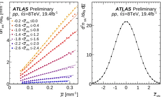
The track density under the peak shown in Fig.1for Mixed events is plotted in the left panel of Fig.2as a function of ¯µfor different ¯z_vtx. Different colors denote different ¯z_vtx. Only several intervals in ¯z_vtx <0 are plotted since there is a symmetry around reduced ¯z_vtx =0. At each ¯z_vtxthe points are fit to a model:

dn_trk/dω∝µ¯ (10)

that reproduces the data with high accuracy. The proportionality coefficients depend on ¯z_vtx and this dependence shown in the right panel can be approximated with a Gaussian shape that has the mean at

-1 ] µ [mm

0 0.1 0.2 0.3

]-1 [mm

ω/dnd trk

0 2 4

6 -0.2 <zvtx ≤0.0

≤-0.4 zvtx

-0.6 <

≤-0.8 zvtx

-1.0 <

≤-1.2 zvtx

-1.4 <

≤-1.6 zvtx

-1.8 <

≤-2.0 zvtx

-2.2 <

≤-2.4 zvtx

-2.6 <

Preliminary ATLAS

=8TeV, 19.4fb-1

s , pp

zvtx

-2 -1 0 1 2

µd

2 ω/dn d trk

0 10 20

Preliminary ATLAS

=8TeV, 19.4fb-1

s , pp

Figure 2: Left: Number of tracks per mm atω=0 as a function of ¯µ. Different marker colors correspond to selected reduced ¯zvtx intervals. Not all intervals are shown for figure clarity. Solid lines are fits assuming scaling of track density with ¯µ. Right: Slopes of the lines shown in the left panel as a function of ¯zvtxfitted to a Gaussian shape.

zero and width very close to unity. This is expected as the ¯z_vtx, according to Eq. (8), is already a reduced parameter. The average number of Background tracks under the peak can be expressed in the form of Eq. (11):

ν≡

n^background_trk =2ωd²n_trk

dωdµ¯G(¯z_vtx) ¯µ, (11)

whereω = 0.75 mm, andd²n_trk/(dωdµ)G(¯¯ z_vtx) is a Gaussian function shown with the solid line in the right panel of Fig.2.

5.4 Properties of Mixed event

The parameters ¯µand ¯z_vtx factorize in Eq. (11). There is only a scaling coefficient betweenνand the interaction densityG(¯z_vtx) ¯µ, such that the sameν can be reached at low instantaneous luminosity and close to the centre of ¯z_vtx interval, or at high instantaneous luminosity and large ¯z_vtx. It can be further assumed that not only the average value, but also the shape of the n_trk distribution in Mixed events is the same for the same interaction densityG(¯z_vtx) ¯µand consequently for the sameν. This assumption is confirmed by the Mixed event taken at different ( ¯µ, ¯z_vtx) and by MC simulations. Events are therefore fully characterized with respect to their background conditions byν, calculated using Eq. (11).

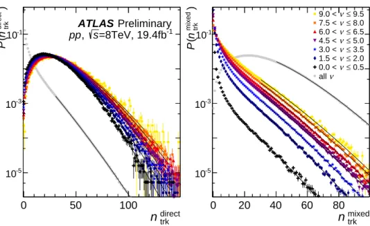
Probability distributions for then_trk found under different νconditions are shown in Fig. 3 for Direct events in the left panel and for Mixed events in the right panel. Different intervals ofνare shown with different marker colors, with darker markers corresponding to condition with lesser background. Grey markers show the averagedn_trk distribution from the other panel shown for comparison. Lines are used to smooth statistical fluctuations.

direct

n

0 100 200

) direct trk n(P

0 0.01 0.02

direct

n trk

0 50 100

) direct trk n(P

10-5

10-3

10-1

Preliminary ATLAS

=8TeV, 19.4fb-1

s , pp

mixed

n trk

0 20 40 60 80

) mixed trk n(P

10-5

10-3

10-1

≤ 9.5 ν 9.0 <

≤ 8.0 ν 7.5 <

≤ 6.5 ν 6.0 <

≤ 5.0 ν 4.5 <

≤ 3.5 ν 3.0 <

≤ 2.0 ν 1.5 <

≤ 0.5 ν 0.0 <

ν all

Figure 3: Probability distributions for thentrkin Direct events (left) and Mixed events (right). Colors correspond to several values ofν. Grey distributions in each panel indicate the distribution from the other panel, averaged over the sample. Lines are fits to data points.

Averaged over the sample,n_trk in Mixed events is below 4, and in Direct events it is above 30. Figure3 shows that the Background tracks affect Direct distributions differently, depending on the n_trk regions.

Assuming that the lower curves, shown with black markers

ν < 0.5

resembles no pileup condition, at n_trk > 100 the Direct events distributions are dominated by Background tracks, rising by an order of magnitude with respect to black curve for the highestνmeasured in the event sample.

Mixed event distributions are shown in the right panel and the common feature of all curves is that above n_trk = 20 they all have similar slope. This suggests that multi-pileup events do not play important role in the measured sample. Rather, the high-ntrktail in Mixed events occurs when a single event falls close to the center of−0.75 < w < 0.75 mm acceptance window. The probability to get a single event in an acceptance interval scales withνand therefore there is a factor of∼7 between the amplitudes of the tails of the two lowest curves, a factor of∼1.9 between the 2^nd and the 3^rd, etc. according to the νshown in the legend. Events with highn_trk should have kinematic distributions close to those of the inclusive ppcollisions. Tracks in them are correlated since most of those tracks are coming from a single pileup interaction. For even higher values ofν, differentνcurves may develop difference in slopes becoming less steep with increasingν, however this regime is not reached in the presently analyzed data.

Analysis of the pileup in [27] showed that the kinematic distributions of the Background changes with background conditions. Since high-ntrk events have higher probability to occur when the pileup inter- action vertex falls at the center of thewacceptance window, low-n_trk events occur when the interaction vertex is closer to the window boundary. According to Eq.7 tracks are more likely to be accepted if they have smallersin(θ), i.e. are the large-ηtracks. For low-pTtracks thez₀parameter is measured with larger uncertainties than for high-p_T tracks and this smearing helps low-p_T tracks from nearby pileup interaction to satisfy|ω| < 0.75 mm. This leads to ann_trk dependence of the kinematic distributions in Mixed events shown in Fig.4. Distributions are averaged over allνin the sample. Theνdependence of the distribution shown in the figure is much weaker than then_trk dependence and is mainly seen for low

Figure 4: Kinematic distribution of tracks in Mixed events for two different ranges of then_trkmeasured in the event.

Distributions are averaged over allνin the sample.

n_trk. Further, the probability that a significant fraction of tracks in Mixed event is coming from a single pileup interaction is higher in events with highn_trkand therefore correlations between tracks are different in high- and low-ntrkMixed events, with the former more strongly correlated.

5.5 Correction forn_trk

The number of Signal tracks can be derived by unfolding then_trkdistributions measured in Direct events.

Transition matrices required for unfolding are constructed from the data using the distributions shown in Fig.3:

M

ν,n^signal_trk ,n^direct_trk

=P_Direct

ν <0.5,n^signal_trk

P_Mixed

ν,n^direct_trk −n^signal_trk

(12) The matrices are using Direct n_trk distribution measured at the lowest ν as the closest proxy for the Signal distribution. This distribution is counted along the "Signal" axis of the matrix. The probability corresponding to eachn_trkvalue is multiplied by the probabilities in the Mixed event distributions shown in the right panel of Fig. 3 corresponding to an interval of ν. The smeared values are counted along the "Direct" axis of the matrix. Where necessary, fits are used to suppress statistical fluctuations. Two examples of transition matrices are shown in Fig.5.

The two matrices correspond to low and high values ofνfound in the data. The contour lines of the matrices have distinct "spinnaker" shape with the amount of "drag" increasing withν. At high "drag" the higher values ofn_trkin Direct events become only weakly correlated to then_trkin Signal events. The right panel of Fig.5shows that the largest number of tracks in Direct corresponds to relatively moderate Signal n_trksmeared by the Background. This effect limits the range to whatn_trk values the pileup data samples can be analyzed, and the limit depends on theνcondition.

M

10-7

10-5

10-3

direct

n trk

0 50 100 150

signal trkn

0 50 100 150

≤ 0.5 ν 0 <

Preliminary ATLAS

=8TeV, 19.4fb-1

s , pp

M

10-7

10-5

10-3

direct

n trk

0 50 100 150

signal trkn

0 50 100 150

≤ 9.5 ν 9 <

Preliminary ATLAS

=8TeV, 19.4fb-1

s , pp

Figure 5: Data-driven transition matrices corresponding to different intervals ofνthat are used for unfolding.

5.6 Correction for the pair-distribution

To derive the 2PC for the Signal, the contribution of the Background has to be removed. Using Eq. (9) one can write:

(Signal×Signal)=(Direct×Direct) − (Mixed×Mixed)− 2

(Direct)×(Mixed) − (Mixed)×(Mixed)

, (13)

where brackets (×) or ( )×( ) denote whether the correlation function is constructed between the tracks in the same event or in two different events respectively. Naturally, in the latter case tracks are uncorre- lated, therefore ( )×( ) terms in the second line can only be constant factors. Due to effects discussed in Section5.4the magnitudes of those terms depend on then_trkin Background events.

Each Direct event with a givenn_trk contains contributions from Signal events with any number of tracks such thatn^signal_trk ≤ n^direct_trk . Those contributions are calculated from the transition matrices shown in Fig.5 by making a projection ofn^direct_trk onton^signal_trk for a given value ofn^signal_trk . These projections are shown in Fig.6for two intervals ofν.

The histograms in the figure are examples of probability distributions of then^signal_trk contributing to fixed number ofn^direct_trk =30,60, and 90. At the lowνshown in the left panel, the distributions are narrow and peaked atn^signal_trk = n^direct_trk . Under such low pileup condition, more than 85% of events do not have even one Background track. The situation is different for highνwhere the contributions to Direct are coming from a wide range of Signal with smallern_trk. Boxes shown in the plot are centered horizontally at the mean values ofn^signal_trk contributing to Direct events and have width equal to 2×RMS of the corresponding distributions. Distributions for high values ofn_trkin Direct events develop a second maximum as shown with the red curve in the right panel. Figure6demonstrates that with increasingνit becomes impossible to accurately determine to what n^signal_trk the measurement belongs. Figure6 shows that the presence of pileup deteriorates the resolution with which one can measuren_trk.

signal

n trk

0 20 40 60 80

) signal trk n(P

0 0.2 0.4 0.6 0.8

1 ^{0 <} ν ≤ 0.5

signal

n trk

0 20 40 60 80

) signal trk n(P

0 0.05 0.1 0.15

≤ 9.5 ν 9 <

trk =30

direct

n

trk =60

direct

n

trk =90

direct

n

Preliminary ATLAS

=8TeV, 19.4fb-1

s , pp

Figure 6: The probability of a Signal track to contribute to an event with 30, 60 and 90 (black, blue and red) Direct tracks. Boxes denote the horizontal range equal to a mean±RMS value of the histogram with corresponding color.

The left panel is for 0<ν<0.5 and the right panel for 9<ν<9.5.

The 2PC do not have strongn_trkdependence and therefore allow the use of wide range ofνconditions,ν≤ 7.5, before contamination is too strong to be corrected for. To measure correlations in Signal events, first the 4 terms of Eq. (13) are constructed. This is done independently for each range ofν. The correlators for (Direct×Direct), (Mixed)×(Mixed), and (Mixed×Mixed) terms are calculated for each number of n_trkin the corresponding samples and the (Direct)×(Mixed) term for all combinations ofn^mixed_trk <n^direct_trk . Then, using distributions like those shown in Fig.6the Background is removed from the (Direct×Direct) term according to Eq. (13). The correlator obtained in this procedure has no Background contribution, but it still remains a measurement inn^direct_trk . It is reassigned ton^signal_trk using again the distributions shown in Fig.6. Than the results measured in differentνconditions are averaged together and grouped into wider n_trkbins.

6 Template fits

Figure7shows the pileup corrected 2PC for two differentn^signal_trk intervals. Correlations are measured for tracks in the 0.5<p^a,b_T <5 GeV range (track multiplicity is measured for p_T > 0.4 GeV). In the higher track multiplicity interval of 70–80, a clear enhancement on the near-side (∆φ=0) is visible. Figure7 also shows results for the template fits to the 2PC, with then^signal_trk interval of 20<n^signal_trk ≤30 used as the peripheral reference. The measured correlation functions are well described by the template fits, with long-range correlations (indicated by dashed blue lines) observed in both cases.

From the template fits thev₂is extracted following Eq. (5). The left panel of Fig.8shows thev₂values obtained from the template fits as a function of n^signal_trk . The v₂ values before correcting for pileup are also shown for comparison. They are plotted as a function ofn^direct_trk . When not correcting for the pileup contribution, a clear monotonic decrease inv₂is observed with increasing track multiplicity corresponding to an increase of pileup contamination. From the right panel of Fig. 8, which shows the ratio of the

φ

∆

0 2 4

)φ∆(C

0.98 1 1.02 1.04

) φ (∆ C

) φ (∆

periph

FC + G

) φ (∆

templ

C

periph(0) FC + G

periph(0) FC

ridge + C

ATLAS Preliminary

=8 TeV, 19.4fb-1

, s pp

<5.0 GeV

b , a

pT

0.5<

|<5.0 η 2.0<|∆

50

signal≤ ntrk

40<

-tagged events Z

φ

∆

0 2 4

)φ∆(C

0.98 1 1.02

) φ (∆ C

) φ (∆

periph

FC + G

) φ (∆

templ

C

periph(0) FC + G

periph(0) FC

ridge + C

ATLAS Preliminary

=8 TeV, 19.4fb-1

, s pp

<5.0 GeV

b , a

pT

0.5<

|<5.0 η 2.0<|∆

80

signal≤ ntrk

70<

-tagged events Z

Figure 7: Template fits to the pileup correctedC(∆φ). The left and right panels correspond to two different track mul- tiplicity intervals. Then^signal_trk ∈(20,30] bin is used to determine theC^periph(∆φ). TheFC^periph(∆φ) andC^ridgeterms have been shifted up byGandFC^periph(0) respectively, for easier comparison. The plots are for 0.5<p^a,b_T <5 GeV.

template-v₂without the pileup correction to with the pileup correction, it is seen that the decrease when not correcting for pileup is∼25% at the highest track multiplicity³. However, after the pileup pairs are removed, thev₂is approximately independent of the track multiplicity, consistent with the observations in Refs. [2,3]).

direct

ntrk signal or ntrk

0 20 40 60 80 100

)a Tp(2v

0 0.05 0.1

Pileup corrected No correction for pileup ATLAS Preliminary Template Fits

=8 TeV, 19.4fb-1

, s pp

-tagged events Z

|<5.0 η 2.0<|∆

<5.0 GeV

,b a

pT

0.5<

direct

ntrk signal or ntrk

0 20 40 60 80 100

ratio: uncorrected/corrected2v 0.8

1 1.2

ATLAS Preliminary Template Fits

=8 TeV, 19.4fb-1

, s pp

-tagged events Z

|<5.0 η 2.0<|∆

<5.0 GeV

,b a

pT

0.5<

Figure 8: Left panel: thev2 values obtained from the template fits when correcting for pileup pairs, plotted as a function of then^signal_trk . Also shown for comparison, are to thev2obtained when not correcting the 2PC for pileup, plotted as function ofn^direct_trk . Right panel: the ratio of the twov2values. Plots are for 0.5<p^a,b_T <5 GeV.

3 Strictly speaking, since the corrected and uncorrectedv2are plotted as functions of different quantities: the corrected track multiplicityn^signal_trk andn^direct_trk , respectively, taking their ratio is not entirely correct. However, it is a good way of illustrating the effect of the correction.

7 Systematic uncertainties

This section discusses the evaluation of the systematic uncertainties in extracting thev₂. The systematics can broadly be classified into two categories: The first are systematics that are intrinsic to the 2PC and to the template fitting procedure and have been used in previous 2PC analyses [2, 28]. These include uncertainties on choosing the peripheral bin used in the template fits, on the tracking efficiency, and on the pair-acceptance. The second category are the uncertainties associated with the correction of thev₂ due to pileup tracks which are specific to the present analysis.

7.1 Peripheral interval

The template fitting procedure assumes that the contributions to the pair distributions from hard pro- cesses have identical shape across all event activity ranges, and only change in overall scale. It also assumes that thev₂only weakly dependends on the event activity. The template fitting procedure uses the n^signal_trk ∈(20,30] interval as the peripheral reference. To test the sensitivity of the measuredv2to any resid- ual changes in the width of the away-side jet peak and to thev₂present in the peripheral reference, the analysis is repeated using the 0–20, 10–20, and 30–40 multiplicity intervals as the peripheral reference, and including the resulting variation in thev2as a systematic uncertainty. This uncertainty varies from

∼7% atn^signal_trk =30 to∼3% forn^signal_trk >70.

7.2 Track reconstruction efficiency

In evaluating the correlation functions, each particle is weighted by factor 1/(p_T, η) to account for the tracking efficiency. The systematic uncertainties in the efficiency(p_T, η) thus need to be propagated into C(∆φ) and the finalv_2,2measurements. TheC(∆φ) andv₂are mostly insensitive to the tracking efficiency.

This is because thev_2,2measures the relative variation of the yields in∆φ; an overall increase or decrease in the efficiency changes the yields but does not affect thev₂. However, due to p_T andηdependence of the tracking efficiency and its uncertainties there is some residual effect on the v₂. The corresponding uncertainty in thev₂ is estimated by repeating the analysis while varying the efficiency to its upper and lower uncertainty extremes. Forv₂this uncertainty is estimated to be 0.5%.

7.3 Pair-acceptance

The analysis relies on the B(∆φ) distribution to correct for the pair-acceptance of the detector using Eq. (2). The B(∆φ) distributions are nearly flat in ∆φ, and the effect on the v2 when correcting for the acceptance in less than 1% for all multiplicities. Since the pair-acceptance corrections are small, the entire correction is conservatively taken as the systematic uncertainty associated with pair-acceptance effects.

7.4 Mixed and Background equivalence

Section5.2demonstrates the equivalence of Mixed events constructed by the random selection procedure to the Background events. The Mixed events are generated from the same sample that containsZbosons.

In order to check possible biases in using theZ-event samples to generate the Mixed events, an alternate set of Mixed events are generated from events selected with a zero-bias trigger, that selects events at random. The result of choosing this alternate sample for the Mixed events results in a variation of at most 2% on thev₂, and is included as a systematic uncertainty.

7.5 Accuracy of the background estimator

This uncertainty arises due to inaccuracy in determination of µ and due to inaccuracy with which ν parameterization reproducing real background. The former is estimated assuming that typical inaccuracy in luminosity determination is about 5%. Sinceνscales withµ, the analysis is repeated withνaltered by the same amount. The background estimatorνis determined using Eq. (11). Although fits used in the functional form of Eq. (11) accurately reproduce data as shown in Figs.1,2alternative fit functions are also studied to derive uncertainty that together with theµinaccuracy results in 1% uncertainty added to the final result.

7.6 Uncertainties in transition matrices

The transition matrices discussed in Section5.5for unfolding then_trkdistributions and for finding coeffi- cients for correcting the 2PC are worked out based on data itself. Then^signal_trk distribution is approximated with the Direct distributions in the lowestνinterval (ν <0.5). Uncertainties on thev₂, due to this approxi- mation are estimated by repeating the analysis with the matrices worked out based on Direct distributions in the intervalν <1 The variation is less than 2% throughout, and is included as a systematic uncertainty on thev₂.

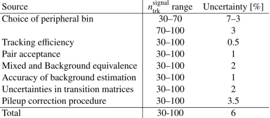
Source n^signal_trk range Uncertainty [%]

Choice of peripheral bin 30–70 7–3

70–100 3

Tracking efficiency 30–100 0.5

Pair acceptance 30–100 1

Mixed and Background equivalence 30–100 2 Accuracy of background estimation 30–100 1 Uncertainties in transition matrices 30–100 2

Pileup correction procedure 30–100 3.5

Total 30-100 6

Table 1: Systematic uncertainties for thev2, given in percent. Where ranges are provided for both multiplicity and the uncertainty, the uncertainty varies from the first value to the second value as the multiplicity varies from the lower to upper limits of the range.

7.7 Accuracy of the pileup correction procedure

As described in Section5, the pileup correction procedure is implemented in intervals ofν. In order to check residual pileup effects that are not corrected by the procedure, a study of the pileup-correctedv₂is performed as a function of theν. This uncertainty may haveν- andn_trk-dependent nature, however given the size of statistics in this data sample a constant conservative±3.5% uncertainty is assigned to thev₂ results.

Table1summarizes the systematic uncertainties given in percent of the measuredv₂values.

8 Results

The left panel of Fig.9 shows the finalv2 values obtained from the template fit in the 8 TeVZ-tagged sample, together with the systematic uncertainties. For comparison, thev₂ values obtained in 13 TeV and 5 TeV inclusive ppcollisions from Ref. [3] are also shown. The right panel shows the ratio of the 8 TeVv2to the 13 TeVv2values. TheZ-tagged 8 TeVv2values show at most a weak dependence on the multiplicity, similar to the results obtained with the inclusive samples. However, theZ-taggedv₂values are slightly larger than the inclusivev₂results. The value averaged over 30–100 multiplicity interval is approximately 8% higher than the inclusive data. This difference is likely to be not due to the difference in √

s, as both the 5 and 13 TeV inclusive v₂ results are consistent with each other, implying an √ s independence of theppv₂. This difference in only a∼ 1.4σdeviation given the systematic uncertainties in the measurements.

signal

ntrk

0 20 40 60 80 100

2v

0.05 0.1

13 TeV inclusive 5 TeV inclusive

-tagged 8 TeV Z

ATLAS Preliminary Template Fits

=8 TeV, 19.4fb-1

, s pp

|<5.0 η 2.0<|∆

<5.0 GeV

b , a

pT

0.5<

signal

ntrk

0 20 40 60 80 100

ratio to 13 TeV inclusive2v 0.8

1 1.2 1.4

-tagged 8 TeV Z

ATLAS Preliminary Template Fits

=8 TeV, 19.4fb-1

, s pp

|<5.0 η 2.0<|∆

<5.0 GeV

b , a

pT

0.5<

Figure 9: Left panel: thev₂ values obtained from the template fits when correcting for pileup pairs, plotted as a function of then^signal_trk . Also shown for comparison, are thev₂obtained in 13 TeV and 5 TeV inclusiveppdata. The error bars and shaded bands indicate statistical and systematic uncertainties, respectively. Right panel: the ratio of thev₂ measured in theZ-tagged 8 TeV to thev₂ measured in the inclusive 13 TeV events. The horizontal dotted line indicates unity and is kept to guide the eye. The horizontal dashed line indicates the average value of the ratio.

Plots are for 0.5<p^a,b_T <5 GeV.

9 Summary

In this analysis, the long-range component (|∆η|>2) of two-particle correlations in √

s = 8 TeV ppcol- lisions that have aZ boson is studied. The dataset corresponds to an integrated luminosity of 19.4 fb⁻¹. The correlations are studied using a template-fitting procedure developed in Refs. [2,3] that separates the genuine long-range correlation from the dijet contribution. Due to the high luminosity conditions, signif- icant contribution to the 2PC from pileup events is observed that contaminates the measured correlations.

To tackle this, a new pileup removal procedure is developed to remove the contribution of pileup tracks.

The pileup corrected 2PC are measured across a large range of track multiplicities and the second order Fourier coefficient of the single-particle anisotropy,v₂, is extracted. The pileup correctedv₂values show only a weak dependence on track multiplicity, quite similar to that observed in inclusive ppcollisions.

The magnitude of the observedv₂is found to be 8±6% larger than thev₂of inclusive ppcollisions.

References

[1] CMS Collaboration,Observation of long-range, near-side angular correlations in proton–proton collisions at the LHC,JHEP09(2010) 091, arXiv:1009.4122.

[2] ATLAS Collaboration,Observation of long-range elliptic anisotropies in √

s=13and 2.76 TeV pp collisions with the ATLAS detector,Phys. Rev. Lett.116(2016) 172301, arXiv:1509.04776.

[3] ATLAS Collaboration,Measurements of long-range azimuthal anisotropies and associated Fourier coefficients for pp collisions at √

s=5.02and 13 TeV and p+Pb collisions at

√s_NN =5.02TeV with the ATLAS detector,Phys. Rev.C96(2017) 024908, arXiv:1609.06213.

[4] CMS Collaboration,

Observation of long-range, near-side angular correlations in pPb collisions at the LHC, Phys. Lett. B718(2013) 795, arXiv:1210.5482.

[5] ATLAS Collaboration,Long-range angular correlations on the near and away side in p+Pb collisions at √

s_NN =5.02TeV,Phys.Lett.B719(2013) 29–41, arXiv:1212.2001.

[6] ATLAS Collaboration,Observation of Associated Near-Side and Away-Side Long-Range Correlations in √

s_NN =5.02TeV Proton–Lead Collisions with the ATLAS Detector, Phys. Rev. Lett.110(2013) 182302, arXiv:1212.5198.

[7] H. Sorge,

Elliptical flow: A Signature for early pressure in ultrarelativistic nucleus-nucleus collisions, Phys. Rev. Lett.78(1997) 2309–2312, arXiv:nucl-th/9610026.

[8] P. Huovinen, P. F. Kolb, U. W. Heinz, P. V. Ruuskanen, and S. A. Voloshin,

Radial and elliptic flow at RHIC: Further predictions,Phys. Lett.B503(2001) 58–64, arXiv:hep-ph/0101136.

[9] P. F. Kolb, U. W. Heinz, P. Huovinen, K. J. Eskola, and K. Tuominen,

Centrality dependence of multiplicity, transverse energy, and elliptic flow from hydrodynamics, Nucl. Phys.A696(2001) 197–215, arXiv:hep-ph/0103234.