The ATLAS Collaboration

ATLAS-CONF-2010-088 11October2010

ATLAS NOTE

ATLAS-CONF-2010-088

August 21, 2010

Search for new physics in multi-body final states at high invariant masses with ATLAS

The ATLAS Collaboration

Abstract

Preliminary results of a search for new physics in multi-body final states in proton-proton

collisions at a centre-of-mass energy of √ s = 7 TeV are presented. The data were collected

in 2010 with the ATLAS detector at the LHC and correspond to an integrated luminosity of

(295 ± 32) nb

⁻¹

. We observe 193 events with at least three objects in the final state and an

invariant mass above 800 GeV and ∑ p

_T

> 700 GeV, in agreement with the Standard Model

prediction of 254 ± 18 ± 84. An upper limit of 0.34 nb, at the 95% confidence level, is

determined for the production cross section times acceptance for new physics models that

result in these final states. The result is of interest for models of low-scale gravity and

weakly-coupled string theory.

1 Introduction

The search for new physics phenomena beyond the Standard Model is a major goal of the ATLAS de- tector. A broad range of models have been developed over the past decades which address questions as yet unanswered in the Standard Model. One of the key issues is the apparent weakness of gravity com- pared to the other known fundamental forces. In other words, why is the Planck scale, M

_Pl

∼ 10

¹⁹

GeV, about sixteen orders of magnitude higher than the electroweak scale? A possible solution to this hier- archy problem is offered by theories with a new gravity scale of about 1 TeV [1–8]. One popular idea postulates a number of extra spatial dimensions. The observed weakness of gravity is then due to the gravitational field propagating into the higher-dimensional space (bulk), while the Standard Model fields are confined to our familiar three-dimensional space (brane) or localised in limited regions of the bulk.

In these models, the fundamental scale of gravity, M

_D

[9], can be in the TeV range, while the Planck scale is an effective scale seen in a three-dimensional world. The relationship between the two scales is model-dependent.

Some low-scale gravity models predict the production of gravitational states close to the new mass scale and continuum production of non-perturbative states above it. For example, the production of black holes [10–12], string balls [6,13], and p-branes [14,15] could occur. In this paper, we search for evidence of such new states. Since the production and decay occurs in the strong-gravity regime and we lack a UV- complete theory of quantum gravity, there are few robust theoretical predictions of their production and decay properties. Well above the gravitational scale, it is anticipated that the semi-classical description of Hawking evaporation [16] and black hole thermodynamics [17–19] will be applicable.

We refer to previous experimental limits [9], to determine the mass scale at which to conduct our search. These limits permit the fundamental scale of gravity to be below 1 TeV, depending on the model assumptions. The lower limit from collider experiments on the fundamental scale M

_D

in ADD models [1–

3] decreases with increasing number of extra dimensions. For six extra dimensions it is 940 GeV [20], while for greater than six extra dimensions it is about 800 GeV [21]. We search in the invariant mass spectrum above 800 GeV.

We rely on a few basic assumptions for the behaviour of final states arising from gravity in the quantum regime. We expect deviations from the Standard Model predictions, in the invariant mass distribution of several high- p

T

objects. It is assumed that gravity couples only to the energy-momentum content of matter and thus the decays of strong-gravitational objects are approximately democratic to all degrees of freedom in the Standard Model. Therefore, we include the detector signatures from the low-mass fundamental objects of the Standard Model in our search: electrons, photons, muons, and jets.

In the semi-classical regime, we expect the decay to involve a large number of high-energy particles.

We make no requirement on the particle types or their number other than the requirement that their total number is greater than two. We attempt to keep the search as general as possible, and be guided only by kinematics in choosing our requirements for reducing the backgrounds. This is the first search of this type.

2 ATLAS detector

The ATLAS detector is a multipurpose apparatus with a nominally forward-backward symmetric cylin-

drical geometry and near 4π coverage in solid angle [22]. The overall layout of the detector is driven

by its four magnet systems: a thin superconducting solenoid surrounding an inner tracking cavity and

three large superconducting toroids (one barrel and two end caps) surrounding the calorimeters with an

eightfold azimuthal symmetry. The calorimeters, which are surrounded by an extensive muon system,

are of particular importance to this analysis. In the pseudo-rapidity region

¹

| η | < 3.2, high-granularity liquid-argon (LAr) electromagnetic sampling calorimeters with very good energy resolution are used.

A scintillator-tile calorimeter provides hadronic coverage in the range |η | < 1.7 and comprises a large central barrel and two smaller extended barrel cylinders, one on each side. The end-cap and forward re- gions, spanning 1.5 < |η| < 4.9, are again instrumented with LAr calorimetry for both electromagnetic and hadronic energy measurements.

3 Data sample, event selection, and object reconstruction

A sample of events was collected corresponding to 295 nb

⁻¹

of proton-proton collisions. A single un-prescaled lowest-level (L1) hardware-based calorimeter jet trigger with a nominal energy threshold of 15 GeV is required. These events are required to have at least five tracks from a reconstructed primary vertex with a z-position within 15 cm of the LHC beam position. This requirement suppresses beam-induced backgrounds and cosmic-ray events. 1% of events are removed by the vertex requirement.

Additional quality criteria are applied to the events to ensure that jets are not produced by single noisy calorimeter cells or problematic detector regions [23].

Jets are reconstructed using the infrared- and collinear-safe anti-k

T

jet clustering algorithm [24] with a radius parameter of 0.4 using energy depositions in topological calorimeter clusters as input [25]. An average correction, determined as a function of jet transverse momentum and pseudo-rapidity, and ex- tracted by numerical inversion from Monte Carlo simulation, is applied to the measured jets to obtain an improved transverse momentum measurement [26]. For object selection, jets with transverse momentum

p

_T

> 40 GeV and pseudo-rapidity |η| < 2.8 are included.

Electron and photon reconstruction is based on clusters of a fixed size in η × φ in the electromagnetic calorimeter. Electrons are reconstructed from the clusters if there is a suitable match with a track of transverse momentum above 0.5 GeV. Photons are reconstructed from the clusters if there is no reconstructed track matched to the cluster (unconverted photon candidates) or if there is a reconstructed conversion vertex matched to the cluster (converted photon candidates).

Electromagnetic objects are selected as follows: electrons and photons with transverse momentum p

T

> 20 GeV, and pseudo-rapidity | η | < 2.47 for electrons and | η | < 2.37 for photons. Electrons and photons in the transition regions of the calorimeter 1.37 < | η | < 1.52 are not identified as electrons and photons, but could be included as jets if they are also identified by the jet reconstruction algorithm.

A combined muon reconstruction algorithm is used in this analysis. This associates a standalone muon spectrometer track with an inner detector track using a χ

²

consistency criterion, based on the difference between the two sets of track parameters weighted by their combined covariance matrix. For the object selection, muons with transverse momentum p

T

> 20 GeV and pseudo-rapidity |η| < 2.0 are included.

The missing transverse energy of the event, E

_T^miss

, is used in the calculation of the invariant mass of the event. It is reconstructed using calorimeter cells belonging to clusters in the pseudo-rapidity range

| η | < 4.8. This cell selection provides efficient noise suppression [27]. The energy of muon candidates is subtracted in the calculation.

The identification of detector signatures as final-state objects can be ambiguous. The same de- tector hits can be reconstructed as two different objects with a small separation in ∆R, where ∆R ≡ p ∆η

²

+ ∆φ

²

, and ∆η (∆φ ) are the differences between the reconstructed pseudo-rapidities (azimuthal

1The ATLAS reference system is a Cartesian right-handed coordinate system, with a nominal collision point at the origin.

The anticlockwise beam direction defines the positive z-axis, while the positive x-axis is defined as pointing from the collision point to the centre of the LHC ring and the positive y-axis points upwards. The azimuthal angleφis measured around the beam axis in the transverse (xy)-plane, and the polar angleθis measured with respect to the z-axis. The pseudo-rapidity is defined as η=−ln(tan(θ/2)).

angles) of the two objects. In such cases, if ∆R < 0.1 between an electron and a photon, or ∆R < 0.2 between a jet, and either an electron or a photon, the ambiguity is resolved by selecting electrons, pho- tons, and jets, in that order of priority. Muons are not included in this procedure, as muons produced close to jets are unlikely to have their energy included in the jet energy. We do not attempt further object identifications, for example to tag taus or heavy-flavour decays, or the reconstruction of heavier states such as W-bosons, Z-bosons, and top quarks. Not reconstructing these objects has no impact on the invariant mass of the event.

4 Standard Model Backgrounds

The dominant Standard Model background for this search is QCD jet production [28]. The predictions for this process are subject to uncertainties. However, the analysis method we use is designed to avoid many of the uncertainties in QCD predictions by extrapolating from a nearby region where no new physics is present. The analysis is sensitive to uncertainties in QCD effects, such as higher-order QCD radiation, showering, and hadronisation. To estimate the effect of hard radiation, two event generators, P

YTHIA

6.421 [29] and A

LPGEN

2.06 [30], are used. P

YTHIA

produces two hard jets using leading- order (LO) matrix elements. High-multiplicity final states appear as a result of QCD shower processes.

In contrast, A

LPGEN

produces up to six hard jets in the final state using leading order QCD matrix element calculations for multi-parton final states, and Mangano (MLM) matching to combine them with parton shower models. A

LPGEN

is combined with J

IMMY

4.3 [31] for the underlying event simulation and H

ERWIG

6.510 [32] for the parton shower simulation and hadronisation. For comparison, we also use the LO implementation of the H

ERWIG

and H

ERWIG

++ 2.4.2 [33] Monte-Carlo event generators. These two generators also use the parton-shower approach to generate initial- and final-state QCD radiation, including colour coherence effects.

Another background source is t ¯t production, which is generated using MC@NLO [34]. In addition, A

LPGEN

is used to simulate potential contributions from W-boson plus jets Standard Model processes.

Previous studies have shown [28] that other backgrounds are much smaller and can be neglected in this analysis.

The ATLAS MC09 P

YTHIA

tune is used as baseline [35]. To study the effects of the uncertainty in describing soft QCD, we use data sets from two alternative tunes of P

YTHIA

: an alternative fragmentation tune and a different underlying-event model [36]. For the alternative underlying event, we use Perugia0 from the set of Perugia tunes [37]. This is a set of tunes using p

_⊥

-ordered showers with P

YTHIA

version 6.4 and CTEQ5L parton distribution functions (PDFs).

Different parton distribution functions are used with these generators. The baseline P

YTHIA

, H

ER

-

WIG

, and H

ERWIG

++ event samples are generated using MRST 2007 LO

^∗

[38], a PDF set specifically tuned to provide a cross section description for a number of Standard Model processes, which are close to the next-to-leading-order (NLO) prediction, by combining it with leading-order matrix elements. For A

LPGEN

simulations, a leading-order PDF set, CTEQ 6 L1 [39], is used. CTEQ 6.6 was used for the MC@NLO t ¯t samples.

The detector response for all the generated Monte Carlo events is simulated by passing them through

a detailed simulation of the ATLAS detector based on the GEANT4 program [40,41]. These detector

simulated events are then reconstructed, selected, and analysed identically to the data.

Multiplicity

2 4 6 8 10 12 14

events

1 10 10

2

10

3

10

4

10

5

10

6

Multiplicity

2 4 6 8 10 12 14

events

1 10 10

2

10

3

10

4

10

5

10

6

L dt = 295 nb

-1

∫

ATLAS Preliminary

Muon(Data) Electron(Data) Photon(Data) Jet(Data)

Muon(Alpgen) Electron(Alpgen) Photon(Alpgen) Jet(Alpgen)

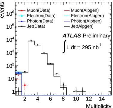
Figure 1: Object multiplicity for events after a requirement of ∑ p

T

> 300 GeV. The markers represent the data and the histograms the background predictions obtained using A

LPGEN

simulations. The jet, electron, photon, and muon distributions are shown in black, cyan, blue, and red respectively.

5 Analysis procedure

5.1 Signal and control regions

We use an analysis strategy that strongly suppresses Standard Model backgrounds, while preserving a high efficiency for a possible high-mass multi-particle final state. We require at least three objects selected according to the criteria in section 3. This reduces low-p

_T

and two-body scattering processes, while having little effect on a potential high invariant mass signal. After the basic event selection, 92527 events with three or more objects remain.

The scalar sum of the transverse momentum of all reconstructed objects in an event,

∑ ^p

^T

^≡ ∑

i=objects

p

Ti

, (1)

is a variable that is strongly correlated to the invariant mass of the event for central production processes.

It is a useful variable for reducing the QCD 2 → 2 scattering amplitudes characterised by a strong forward

peak in the differential cross section, as it selects more centrally produced objects, reducing our exposure

to jet systematics from the forward region. Figure 1 shows the multiplicities of each type of object in

events after a requirement of ∑ p

_T

> 300 GeV for data and the simulated background. The events are

dominated by jets, with a tiny admixture of electrons, photons, and muons. Most common are three

jet events, with those containing four and five jets also significant. Requiring ∑ p

_T

> 300 GeV, selects

11664 events with more than two objects. On visual inspection, the two events in the high-multiplicity

tail were found to be non-collision background events. Further work will be undertaken to study and

reduce this potential background. These two events are removed by the requirements we impose on the

signal events.

We search for an excess of events in the high invariant mass of the final state calculated from all objects in the event using the formula

M

_inv

= p

p

²

and p = ∑

i=objects

p

_i

+ (E

_T^miss

,E

_{T x}^miss

,E

_{T y}^miss

, 0) , (2) where p

_i

is the reconstructed four-momenta of the objects and E

_T^miss

is the missing transverse energy in the event, and E

_{T x}^miss

and E

_{T y}^miss

are the x- and y-components, respectively. A good mass reconstruction is obtained by summing momenta of the reconstructed objects above certain thresholds and including the missing transverse energy. When summing reconstructed objects, it is important to include all identified objects, and to avoid double counting the energy from overlapping objects, as described in section 3.

Due to finite mass resolution effects and the steeply falling parton distribution functions with increas- ing parton centre-of-mass energy, there is considerable migration of events from their true mass values to the reconstructed ones. Our final result is based on counting events above the reconstructed mass threshold of 800 GeV after a requirement of ∑ p

T

> 700 GeV, and is presented as a cross section times acceptance.

Since the cross sections for Monte Carlo simulations can only approximate the true multi-jet cross section, the Monte Carlo samples are normalised to the number of observed events in a control region, where no new physics effects are expected. The method we use is designed to reduce the uncertain- ties in QCD predictions by extrapolating from a nearby control region, and hence, we only rely on the simulation of the shape of the differential cross section in mass.

A grid of possible control regions is studied. A minimum ∑ p

_T

requirement ranging from 200 GeV to 400 GeV, and minimum invariant mass of 200 GeV to 500 GeV, with each being varied in 100 GeV steps are examined. The maximum invariant mass of the chosen control region is 800 GeV in all cases.

A control region consisting of an invariant mass range between 300 GeV and 800 GeV, and a mild ∑ p

_T

requirement of 300 GeV is chosen. This region provides adequate Monte Carlo statistics in a similar kinematic regime to the signal region. In the case of A

LPGEN

, using an adjacent control region changes the predicted number of events in the signal region by less than 2.4%. The P

YTHIA

, H

ERWIG

, and H

ERWIG

++ predictions vary more dramatically across the possible control regions resulting in changes in the predicted number of events in the signal region by up to about 10%, 20%, and 20%, respectively.

We take 10% as a systematic uncertainty on the estimated background due to our choice of control region. In the control region, there are 9215 data events, containing a total of 31454 jets, 17 electrons, 26 photons, and 24 muons.

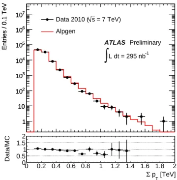
Figure 2 shows the ∑ p

_T

distribution for data and the simulated background after requiring at least three objects in the event. The A

LPGEN

predictions have been normalised to data in the region ∑ p

_T

>

300 GeV and 300 < M

inv

< 800 GeV.

The normalisation of the background is performed by scaling the A

LPGEN

prediction for the cross section by a factor of 1.15 and the P

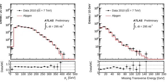
YTHIA

predictions by a factor of 0.64, respectively. Figure 3 shows the object transverse momentum distribution and missing transverse energy distribution for events in the control region compared to A

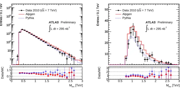
LPGEN

, when normalised to data in the control region. A comparison of the invariant mass from A

LPGEN

, P

YTHIA

, and data for the control and signal regions are displayed in Figure 4.

The signal region, ∑ p

T

> 700 GeV and M

inv

> 800 GeV, contains 193 events. These events contain

769 jets, and no electrons, photons, or muons. After rescaling using the events in the control region,

A

LPGEN

predicts 254 ± 18 events, while P

YTHIA

predicts 174 ± 11 events, where the uncertainties are

due to the limited statistics of the Monte Carlo simulations.

Multiplicity

2 4 6 8 10 12 14

events

1 10 10

2

10

3

10

4

10

5

10

6

Multiplicity

2 4 6 8 10 12 14

events

1 10 10

2

10

3

10

4

10

5

10

6

L dt = 295 nb

-1

∫

ATLAS Preliminary

Muon(Data) Electron(Data) Photon(Data) Jet(Data)

Muon(Alpgen) Electron(Alpgen) Photon(Alpgen) Jet(Alpgen)

0 20 40 60 80 100 120 140 160 180 200

Entries / 10 GeV

1 10 102

103

104

105

106

0 20 40 60 80 100 120 140 160 180 200

Entries / 10 GeV

1 10 102

103

104

105

106

= 7 TeV) s

Data 2010 ( Alpgen

L dt = 295 nb-1

∫

ATLAS Preliminary

Missing Transverse Energy [GeV]

0 20 40 60 80 100 120 140 160 180 200

Data/MC

0 1 2

3^{0 50} 100 150 200 250 300 350 400 450 500

Entries / 25 GeV

1 10 102

103

104

105

106

0 50 100 150 200 250 300 350 400 450 500

Entries / 25 GeV

1 10 102

103

104

105

106 Data 2010 ( s = 7 TeV) Alpgen

L dt = 295 nb-1

∫

ATLAS Preliminary

[GeV]

pT

0 50 100 150 200 250 300 350 400 450 500

Data/MC

0 0.5 1 1.5

20 0.2 0.4 0.6 0.8 1 1.2 1.4 1.6 1.8 2

Entries / 0.1 TeV

1 10 102

103

104

105

106

107

0 0.2 0.4 0.6 0.8 1 1.2 1.4 1.6 1.8 2

Entries / 0.1 TeV

1 10 102

103

104

105

106

107

= 7 TeV) s

Data 2010 ( Alpgen

L dt = 295 nb-1

∫

ATLAS Preliminary

[TeV]

pT

Σ

0 0.2 0.4 0.6 0.8 1 1.2 1.4 1.6 1.8 2

Data/MC

0 0.5 1 1.5 2

Figure 2: Distribution of the scalar sum of the transverse momenta of all objects in the event, after requiring at least three objects in the event. The solid black dots represent the data and the red histogram the background prediction obtained using A

LPGEN

simulation. The lower panel shows the ratio of the data to the A

LPGEN

predictions (solid black dots). The simulated background is scaled to the number of data events in a control region ∑ p

T

> 300 GeV and 300 GeV < M

inv

< 800 GeV.

5.2 Background Uncertainties

The background estimation is subject to three major uncertainties due to: QCD radiation and fragmenta- tion effects; parton distribution functions; and jet-energy scale and jet-energy resolution uncertainties.

In order to estimate the uncertainty due to QCD effects, the predictions of A

LPGEN

, P

YTHIA

, H

ER

-

WIG

, and H

ERWIG

++ were compared with each other. We studied our sensitivity to some of the parame- ters used in QCD simulations, by using an alternative fragmentation tune and different underlying-event model. The different fragmentation tune gives a 0.1% increase in the number of events in the signal region. The Perugia0 tune which contains a different underlying event model, results in a 10% increase in the number of events in the signal region.

For the background estimate, the A

LPGEN

prediction is used, as it better represents multiple hard jets and is more stable with respect to changes in the control region. A

LPGEN

and P

YTHIA

bracket the range of background predictions in the signal region, include the H

ERWIG

and H

ERWIG

++ predictions, and P

YTHIA

predictions for two alternative tunes. The difference in the predictions between A

LPGEN

and P

YTHIA

, re-weighted to the CTEQ 6L1 PDFs used by A

LPGEN

, is taken as a systematic uncertainty on the background due to QCD effects. Our best estimate of the background is 254 ± 18 ± 67 events, where the former uncertainty is the statistical uncertainty, and the latter the systematic uncertainty due to QCD modelling.

The uncertainty due to PDFs is estimated as follows. The events generated with A

LPGEN

are re-

weighted according to the Bjorken-x values of the interacting partons from the production process and

its scale Q

²

, as given by CTEQ 6L1 to the CTEQ 6.6 central next-to-leading order set. The full set of error

eigenvectors of CTEQ 6.6 are combined following the recipe of Ref. [42] to estimate the spread of next-

Multiplicity

2 4 6 8 10 12 14

events

1 10 102

103

104

105

106

Multiplicity

2 4 6 8 10 12 14

events

1 10 102

103

104

105

106

L dt = 295 nb-1

∫

ATLAS Preliminary Muon(Data)

Electron(Data) Photon(Data) Jet(Data)

Muon(Alpgen) Electron(Alpgen) Photon(Alpgen) Jet(Alpgen)

0 20 40 60 80 100 120 140 160 180 200

Entries / 10 GeV

1 10 102

103

104

105

106

0 20 40 60 80 100 120 140 160 180 200

Entries / 10 GeV

1 10 102

103

104

105

106

= 7 TeV) s Data 2010 ( Alpgen

L dt = 295 nb-1

∫

ATLAS Preliminary

Missing Transverse Energy [GeV]

0 20 40 60 80 100 120 140 160 180 200

Data/MC 0

1 2

30 50 100 150 200 250 300 350 400 450 500

Entries / 25 GeV

1 10 102

103

104

105

106

0 50 100 150 200 250 300 350 400 450 500

Entries / 25 GeV

1 10 102

103

104

105

106 Data 2010 (s = 7 TeV) Alpgen

L dt = 295 nb-1

∫

ATLAS Preliminary

[GeV]

pT

0 50 100 150 200 250 300 350 400 450 500

Data/MC 0

0.5 1 1.5 2

Multiplicity

2 4 6 8 10 12 14

events

1 10 102

103

104

105

106

Multiplicity

2 4 6 8 10 12 14

events

1 10 102

103

104

105

106

L dt = 295 nb-1

∫

ATLAS Preliminary Muon(Data)

Electron(Data) Photon(Data) Jet(Data)

Muon(Alpgen) Electron(Alpgen) Photon(Alpgen) Jet(Alpgen)

0 20 40 60 80 100 120 140 160 180 200

Entries / 10 GeV

1 10 102

103

104

105

106

0 20 40 60 80 100 120 140 160 180 200

Entries / 10 GeV

1 10 102

103

104

105

106

= 7 TeV) s Data 2010 ( Alpgen

L dt = 295 nb-1

∫

ATLAS Preliminary

Missing Transverse Energy [GeV]

0 20 40 60 80 100 120 140 160 180 200

Data/MC 0

1 2 3

Figure 3: Transverse momentum of all objects (left) and missing transverse energy in events (right) for events in the control region ∑ p

_T

> 300 GeV and 300 GeV < M

_inv

< 800 GeV. The solid black dots are the data, while the red histograms are the background predictions using A

LPGEN

normalised to data in the control region. The lower panels show the ratio of the data to the A

LPGEN

predictions (solid black dots).

to-leading order predictions, giving an upper and lower uncertainty on the central CTEQ 6.6 distribution.

Then each of these three distributions are normalised to the data in the control region of ∑ p

T

> 300 GeV and 300 < M

inv

< 800 GeV, and the resulting expectation in the signal region determined. Compared to the number of events predicted using CTEQ 6L1, CTEQ 6.6 predicts 1% more events for its central set, and variations of +7% and − 5% from the central set due to the PDF error sets. The differences due to the error sets are added in quadrature to the other systematic uncertainties and used as an uncertainty in our estimate of the background due to PDF uncertainties. In addition, the A

LPGEN

events are re- weighted to the MRST 2007 LO

^∗

PDF set that is used by P

YTHIA

. The predicted number of A

LPGEN

events decreases by 12% after the re-weighting. This difference is used as an additional uncertainty in our estimate of the background due to different model assumptions among the different PDF groups.

The uncertainty due to the jet-energy scale is estimated using a rapidity and transverse-momentum dependent rescaling function [43–45]. This depends upon the number of vertices reconstructed (with 5 or more tracks). For each Monte Carlo event, a number of vertices was selected according to the distribution from data and the corresponding jet energy scale uncertainty used. For the case of no additional vertex, the overall uncertainty of the jet-energy scale is below 9% over the entire range of p

T

and η considered, and below 7% for central jets with p

_T

> 60 GeV. The effect of the jet-energy scale uncertainty on the predicted background is +6% and − 7%. Concordant numbers are obtained for the A

LPGEN

and P

YTHIA

samples.

Since the topology of the analysed events differs from those used to obtain the energy uncertainty function, an additional uncertainty due to the different response between quark and gluon jets is added linearly to all the jets. Including this additional uncertainty changes the predicted background in total by +7% and − 8%.

An additional uncertainty due to jets close to each other is added linearly to the jet-energy uncertainty.

For those jets with another jet within ∆R < 1, this additional correction is applied. The correction is

independent of p

_T

and η . We take the size of the response correction (4%) as the systematic uncertainty

due to close-by soft jets. Including this additional uncertainty, changes the predicted background by

Multiplicity

2 4 6 8 10 12 14

events

1 10 102

103

104

105

106

Multiplicity

2 4 6 8 10 12 14

events

1 10 102

103

104

105

106

L dt = 295 nb-1

∫

ATLAS Preliminary Muon(Data)

Electron(Data) Photon(Data) Jet(Data)

Muon(Alpgen) Electron(Alpgen) Photon(Alpgen) Jet(Alpgen)

0 20 40 60 80 100 120 140 160 180 200

Entries / 10 GeV

1 10 102

103

104

105

106

0 20 40 60 80 100 120 140 160 180 200

Entries / 10 GeV

1 10 102

103

104

105

106

= 7 TeV) s Data 2010 ( Alpgen

L dt = 295 nb-1

∫

ATLAS Preliminary

Missing Transverse Energy [GeV]

0 20 40 60 80 100 120 140 160 180 200

Data/MC 0

1 2

30 50 100 150 200 250 300 350 400 450 500

Entries / 25 GeV

1 10 102

103

104

105

106

0 50 100 150 200 250 300 350 400 450 500

Entries / 25 GeV

1 10 102

103

104

105

106 Data 2010 (s = 7 TeV) Alpgen

L dt = 295 nb-1

∫

ATLAS Preliminary

[GeV]

pT

0 50 100 150 200 250 300 350 400 450 500

Data/MC 0

0.5 1 1.5

20 0.2 0.4 0.6 0.8 1 1.2 1.4 1.6 1.8 2

Entries / 0.1 TeV

1 10 102

103

104

105

106

107

0 0.2 0.4 0.6 0.8 1 1.2 1.4 1.6 1.8 2

Entries / 0.1 TeV

1 10 102

103

104

105

106

107

= 7 TeV) s Data 2010 ( Alpgen

L dt = 295 nb-1

∫

ATLAS Preliminary

[TeV]

pT

Σ 0 0.2 0.4 0.6 0.8 1 1.2 1.4 1.6 1.8 2

Data/MC 0

0.5 1 1.5

20 0.5 1 1.5 2 2.5 3

Entries / 0.1 TeV

1 10 102

103

104

105

106

0 0.5 1 1.5 2 2.5 3

Entries / 0.1 TeV

1 10 102

103

104

105

106

= 7 TeV) s Data 2010 ( Alpgen Pythia

L dt = 295 nb-1

∫

ATLAS Preliminary

[TeV]

MInv

0 0.5 1 1.5 2 2.5 3

Data/MC 0

0.5 1 1.5

2 0 0.5 1 1.5 2 2.5 3

Entries / 0.1 TeV

10 20 30 40 50

0 0.5 1 1.5 2 2.5 3

Entries / 0.1 TeV

10 20 30 40

50 Data 2010 (s = 7 TeV) Alpgen

Pythia

L dt = 295 nb-1

∫

ATLAS Preliminary

[TeV]

MInv

0 0.5 1 1.5 2 2.5 3

Data/MC 0

1 2 3

Figure 4: Invariant mass distribution for ∑ p

T

> 300 GeV (left) and ∑ p

T

> 700 GeV (right), after nor- malising the background to data in the control region. The solid black dots are the data, while the red and blue histograms are the background predictions obtained using A

LPGEN

and P

YTHIA

, respectively. The lower panels show the ratio of the data to the A

LPGEN

predictions (solid red squares) and the P

YTHIA

predictions (solid blue triangles).

± 11%.

The event pile-up, where more than one proton-proton interaction occur at the same bunch-crossing, introduces additional uncertainties. Fewer than 0.2% of the events in the control region have a jet from a second vertex, so we expect fewer than one event in the signal region. Pile-up can also effect the uncertainty of the jet energy scale. Studies of events with multiple reconstructed primary vertices show that jet energies may acquire an additional energy depending on jet pseudo-rapidity η and number of additional vertices. The average contribution is about 0.5 GeV per each additional primary vertex for

|η| < 1.9, and about 2 GeV for larger |η | . The effect of pile-up was evaluated by subtracting these average contributions from each jet in the data. The effect on the control and signal region is − 3% and

− 4%, respectively .

The propagation of the jet energy scale uncertainty to E

_T^miss

, used in the calculation of the invariant mass, holds an additional uncertainty. The jet energy scale uncertainty is propagated to E

_T^miss

by subtract- ing the original jets and adding back the modified ones. The difference between the predicted number of events in the signal region after this procedure is less than 0.5% compared with that calculated with no change to E

_T^miss

. This difference is included as an additional uncertainty. A further E

_T^miss

uncertainty due to the energy measured outside of reconstructed jets is negligible, since the total energy in the calorimeter is dominated by jets.

There is a possible uncertainty in the number of estimated background events due to the uncertainty in the jet-energy resolution. To estimate the effect of jet-energy resolution uncertainty, we use the bisector raw resolution approach [46]. The jet-energy resolution is 14% [46] for jets with p

_T

values between 20 GeV and 80 GeV, which is conservative for more highly energetic jets. We add additional Gaussian smearing to the jet transverse momentum, and repeat the analysis to study the change in the number of predicted background events. The number of predicted signal events increases by 0.6%. We assigned a 0.6% additional systematic uncertainty to the estimated number of background events due to the jet- energy resolution.

Additional uncertainties of the background estimation arise from other Standard Model contributions

Multiplicity

2 4 6 8 10 12 14

events

1 10

Multiplicity

2 4 6 8 10 12 14

events

1 10

L dt = 295 nb-1

∫

ATLAS Preliminary Muon(Data)

Electron(Data) Photon(Data) Jet(Data)

Muon(Alpgen) Electron(Alpgen) Photon(Alpgen) Jet(Alpgen)

0 20 40 60 80 100 120 140 160 180 200

Entries / 10 GeV

1 10 102

103

104

105

106

0 20 40 60 80 100 120 140 160 180 200

Entries / 10 GeV

1 10 102

103

104

105

106

= 7 TeV) s Data 2010 ( Alpgen

L dt = 295 nb-1

∫

ATLAS Preliminary

Missing Transverse Energy [GeV]

0 20 40 60 80 100 120 140 160 180 200

Data/MC 0

1 2

30 50 100 150 200 250 300 350 400 450 500

Entries / 25 GeV

1 10 102

103

104

105

106

0 50 100 150 200 250 300 350 400 450 500

Entries / 25 GeV

1 10 102

103

104

105

106 Data 2010 (s = 7 TeV) Alpgen

L dt = 295 nb-1

∫

ATLAS Preliminary

[GeV]

pT

0 50 100 150 200 250 300 350 400 450 500

Data/MC 0

0.5 1 1.5

20 0.2 0.4 0.6 0.8 1 1.2 1.4 1.6 1.8 2

Entries / 0.1 TeV

1 10 102

103

104

105

106

107

0 0.2 0.4 0.6 0.8 1 1.2 1.4 1.6 1.8 2

Entries / 0.1 TeV

1 10 102

103

104

105

106

107

= 7 TeV) s Data 2010 ( Alpgen

L dt = 295 nb-1

∫

ATLAS Preliminary

[TeV]

pT

Σ 0 0.2 0.4 0.6 0.8 1 1.2 1.4 1.6 1.8 2

Data/MC 0

0.5 1 1.5

20 0.5 1 1.5 2 2.5 3

Entries / 0.1 TeV

1 10 102

103

104

105

106

0 0.5 1 1.5 2 2.5 3

Entries / 0.1 TeV

1 10 102

103

104

105

106

= 7 TeV) s Data 2010 ( Alpgen Pythia

L dt = 295 nb-1

∫

ATLAS Preliminary

[TeV]

MInv

0 0.5 1 1.5 2 2.5 3

Data/MC 0

0.5 1 1.5

20 0.5 1 1.5 2 2.5 3

Entries / 0.1 TeV

10 20 30 40 50 60

0 0.5 1 1.5 2 2.5 3

Entries / 0.1 TeV

10 20 30 40 50

60 Data 2010 (s = 7 TeV) Alpgen

Pythia

L dt = 295 nb-1

∫

ATLAS Preliminary

[TeV]

MInv

0 0.5 1 1.5 2 2.5 3

Data/MC 0

1 2

3^{0 0.5 1 1.5 2 2.5 3}

Entries / 0.1 TeV

1 10 102

103

104

105

106

0 0.5 1 1.5 2 2.5 3

Entries / 0.1 TeV

1 10 102

103

104

105

106

= 7 TeV) s Data 2010 ( Alpgen

L dt = 295 nb-1

∫

ATLAS Preliminary

[TeV]

MInv

0 0.5 1 1.5 2 2.5 3

Data/MC 0

0.5 1 1.5 2

[TeV]

MInv

0 0.5 1 1.5 2 2.5 3

Data/MC 0

0.5 1 1.5 2

Multiplicity

2 4 6 8 10 12 14

events

1 10

Multiplicity

2 4 6 8 10 12 14

events

1 10

L dt = 295 nb-1

∫

ATLAS Preliminary Muon(Data)

Electron(Data) Photon(Data) Jet(Data)

Muon(Alpgen) Electron(Alpgen) Photon(Alpgen) Jet(Alpgen)

0 20 40 60 80 100 120 140 160 180 200

Entries / 10 GeV

1 10 102

103

104

105

106

0 20 40 60 80 100 120 140 160 180 200

Entries / 10 GeV

1 10 102

103

104

105

106

= 7 TeV) s Data 2010 ( Alpgen

L dt = 295 nb-1

∫

ATLAS Preliminary

Missing Transverse Energy [GeV]

0 20 40 60 80 100 120 140 160 180 200

Data/MC 0

1 2

30 50 100 150 200 250 300 350 400 450 500

Entries / 25 GeV

1 10 102

103

104

105

106

0 50 100 150 200 250 300 350 400 450 500

Entries / 25 GeV

1 10 102

103

104

105

106 Data 2010 (s = 7 TeV) Alpgen

L dt = 295 nb-1

∫

ATLAS Preliminary

[GeV]

pT

0 50 100 150 200 250 300 350 400 450 500

Data/MC 0

0.5 1 1.5

20 0.2 0.4 0.6 0.8 1 1.2 1.4 1.6 1.8 2

Entries / 0.1 TeV

1 10 102

103

104

105

106

107

0 0.2 0.4 0.6 0.8 1 1.2 1.4 1.6 1.8 2

Entries / 0.1 TeV

1 10 102

103

104

105

106

107

= 7 TeV) s Data 2010 ( Alpgen

L dt = 295 nb-1

∫

ATLAS Preliminary

[TeV]

pT

Σ 0 0.2 0.4 0.6 0.8 1 1.2 1.4 1.6 1.8 2

Data/MC 0

0.5 1 1.5

20 0.5 1 1.5 2 2.5 3

Entries / 0.1 TeV

1 10 102

103

104

105

106

0 0.5 1 1.5 2 2.5 3

Entries / 0.1 TeV

1 10 102

103

104

105

106

= 7 TeV) s Data 2010 ( Alpgen Pythia

L dt = 295 nb-1

∫

ATLAS Preliminary

[TeV]

MInv

0 0.5 1 1.5 2 2.5 3

Data/MC 0

0.5 1 1.5

20 0.5 1 1.5 2 2.5 3

Entries / 0.1 TeV

10 20 30 40 50 60

0 0.5 1 1.5 2 2.5 3

Entries / 0.1 TeV

10 20 30 40 50

60 Data 2010 (s = 7 TeV) Alpgen

Pythia

L dt = 295 nb-1

∫

ATLAS Preliminary

[TeV]

MInv

0 0.5 1 1.5 2 2.5 3

Data/MC 0

1 2

3^{0 0.5 1 1.5 2 2.5 3}

Entries / 0.1 TeV

1 10 102

103

104

105

106

0 0.5 1 1.5 2 2.5 3

Entries / 0.1 TeV

1 10 102

103

104

105

106

= 7 TeV) s Data 2010 ( Alpgen

L dt = 295 nb-1

∫

ATLAS Preliminary

[TeV]

MInv

0 0.5 1 1.5 2 2.5 3

Data/MC 0

0.5 1 1.5 2

[TeV]

MInv

0 0.5 1 1.5 2 2.5 3

Data/MC 0

0.5 1 1.5

20 0.5 1 1.5 2 2.5 3

Entries / 0.1 TeV

10 20 30 40 50 60

0 0.5 1 1.5 2 2.5 3

Entries / 0.1 TeV

10 20 30 40 50 60

= 7 TeV) s Data 2010 ( Alpgen

L dt = 295 nb-1

∫

ATLAS Preliminary

[TeV]

MInv

0 0.5 1 1.5 2 2.5 3

Data/MC 0

0.5 1 1.5 2

[TeV]

MInv

0 0.5 1 1.5 2 2.5 3

Data/MC 0

0.5 1 1.5 2

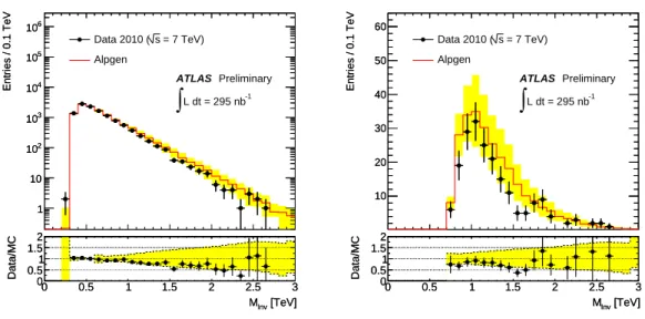
Figure 5: Invariant mass distributions for (left) ∑ p

T

> 300 GeV and (right) ∑ p

T

> 700 GeV. The solid black dots are the data and the red histograms are the background predictions obtained using A

LPGEN

simulation. The background prediction is scaled to the number of data events in a control region ∑ p

_T

>

300 GeV and 300 < M

inv

< 800 GeV, after requiring at least three objects in the event. The error band on the background is the total uncertainty: statistical (negligible) and all systematic uncertainties added in quadrature. The lower panels show the ratio of the data to the background predictions (solid black dots) and the same error band on the background (yellow).

to the background. These contributions are anticipated to be negligible, with the highest contribution estimated to be from top-quark production, W-boson plus jets, and Z-boson plus jets [28]. Their con- tribution of 1.5 events in the signal region is small, and is treated as an additional systematic uncertainty on the background determination due to Standard Model processes that we have not explicitly included.

The number of background events, including all uncertainties, is estimated to be 254 ± 18 ± 84, where the first uncertainty is statistical and the second systematic. All uncertainties on the background estimate are added in quadrature to obtain an overall background uncertainty of ± 34%, including statis- tical and systematic contributions. Figure 5 shows reconstructed invariant mass distributions for data and simulated background after normalising A

LPGEN

to the control region. The error band on the simulated background corresponds to the total uncertainty.

6 Experimental results

A summary of all the numerical results can be found in Table 1. After all the event selections, we observe 193 events above an invariant mass of 800 GeV and with ∑ p

T

> 700 GeV. The observed number of events is consistent with the estimated background of 254 ± 18 ± 84 events; the first uncertainty is statistical and the second uncertainty is systematic. An 11% systematic uncertainty is assigned to the luminosity value obtained from van der Meer beam scans [47]. Based on these numbers of events and an integrated luminosity of (295 ± 32) nb

⁻¹

, we calculate an upper limit on the production cross section times acceptance

²

. Using a Bayesian approach and assuming a flat prior p.d.f. for the signal events, we obtain an upper limit of 0.34 nb, at the 95% confidence level. If we subtract the additional contribution due to pile-up from data, we obtain an upper limit of 0.32 nb.

2The cross-section limit is calculated as usual, with the assumption of 100% acceptance.

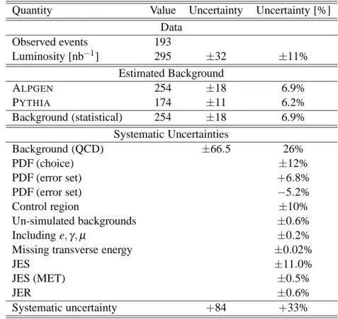
Table 1: Summary of the numerical results. The QCD background systematic is the difference between A

LPGEN

and P

YTHIA

, after re-weighting to the same PDF, as described in section 4.

Quantity Value Uncertainty Uncertainty [%]

Data

Observed events 193

Luminosity [nb

⁻¹

] 295 ± 32 ± 11%

Estimated Background

A

LPGEN

254 ± 18 6.9%

P

YTHIA

174 ± 11 6.2%

Background (statistical) 254 ± 18 6.9%

Systematic Uncertainties

Background (QCD) ± 66.5 26%

PDF (choice) ± 12%

PDF (error set) +6.8%

PDF (error set) − 5.2%

Control region ± 10%

Un-simulated backgrounds ± 0.6%

Including e,γ, µ ± 0.2%

Missing transverse energy ± 0.02%

JES ± 11.0%

JES (MET) ± 0.5%

JER ± 0.6%

Systematic uncertainty +84 +33%

7 Discussion

For an estimation of detector acceptance for high invariant-mass states in low-scale gravity models, we generated Monte Carlo event samples using the event generators C

HARYBDIS

2 [48] and B

LACK

-

MAX

2 [49,50].

In this analysis, we search for multi-body final states with invariant mass above 800 GeV. Since the experimental limit on the Planck scale in ADD models is 800 GeV, or higher depending on the model parameters, the validity of the physics models used in the above generators is questionable for masses close to the Planck scale. However, the above event generators provide a means of simulating the kinematic characteristics of high invariant mass multi-object final states. Several different samples are generated with a range of decay topologies.

We generated three black hole samples using C

HARYBDIS

with fixed decay multiplicities of three, four, and five primary particles. In addition, we generated a B

LACKMAX

event sample using its final burst model [49,50]. All the samples are produced with an energy threshold equal to the Planck scale of 800 GeV and six extra dimensions. The samples are produced with CTEQ 6.6 PDF [51]. These are interfaced to P

YTHIA

for the simulation of QCD effects including parton showers, underlying event, and hadronisation. Subsequently, all the samples are passed through the simulation of the detector response and the event reconstruction.

Using the B

LACKMAX

sample, the acceptance after all selection requirements and for a reconstructed invariant mass above 800 GeV is (58 ± 2)%, where the uncertainty is due to the limited statistics of the Monte Carlo simulated sample. The three C

HARYBDIS

samples give similar acceptances to B

LACKMAX

to within 4%. In spite of good agreement between the simulated signal acceptances, the systematic

uncertainty in the acceptance is expected to be large due to the lack of a well established physics model in the mass region near the gravity scale. Using the BlackMax acceptance value as an illustration, the upper limit on the production cross section for high invariant mass events above 800 GeV is 0.6 nb.

In the most optimistic calculation, the maximum black hole cross-section, can be O (100) nb [48,49], considering the geometric cross section at a mass threshold of 800 GeV. Our illustrative upper limit is well below this value.

This search is less sensitive to cases with large missing energy produced by scenarios involving black hole remnants, significant gravitational radiation in the production process or graviton emission in the decay.

Further searches may produce more restrictive limits by making more specific model assumptions.

For example, the Standard Model background can be strongly suppressed by a requirement of at least one electron or muon in the final state [28]. Assuming an approximately democratic decay of strong- gravitational objects, this would provide a high efficiency for the signal. The transverse momentum requirements will need to be optimised to reduce small angle QCD scattering when the search is per- formed at higher invariant masses.

8 Summary

Preliminary results of a first search for exotic multi-body final states at high invariant masses are pre- sented. The analysis used proton–proton collisions at a centre-of-mass energy of 7 TeV recorded with the ATLAS detector at the LHC. The data were collected in 2010 and correspond to an integrated luminosity of 295 nb

⁻¹

. We observe 193 events with at least three particles in the final state and an invariant mass above 800 GeV and ∑ p

T

> 700 GeV in agreement with the Standard Model prediction of 254 ± 18 ± 84.

An upper limit of 0.34 nb, at the 95% confidence level, is determined for the production cross section times acceptance for new physics models that result in these final states. The result is of interest for models of low-scale gravity and weakly-coupled string theory.

References

[1] N. Arkani-Hamed, S. Dimopoulos, and G. R. Dvali, The hierarchy problem and new dimensions at a millimeter, Phys. Lett. B 429 (1998) 263. arXiv:hep-ph/9803315.

[2] I. Antoniadis, N. Arkani-Hamed, S. Dimopoulos, and G. R. Dvali, New dimensions at a millimeter to a Fermi and superstrings at a TeV, Phys. Lett. B 436 (1998) 257. arXiv:hep-ph/9804398.

[3] N. Arkani-Hamed, S. Dimopoulos, and G. R. Dvali, Phenomenology, astrophysics and cosmology of theories with sub-millimeter dimensions and TeV scale quantum gravity, Phys. Rev. D 59 (1999) 086004. arXiv:hep-ph/9807344.

[4] L. Randall and R. Sundrum, A large mass hierarchy from a small extra dimension, Phys. Rev. Lett.

83 (1999) 3370. arXiv:hep-ph/9905221.

[5] L. Randall and R. Sundrum, An alternative to compactification, Phys. Rev. Lett. 83 (1999) 4690.

arXiv:hep-th/9906064.

[6] S. Dimopoulos and R. Emparan, String balls at the LHC and beyond, Phys. Lett. B 526 (2002) 393. arXiv:hep-ph/0108060.

[7] G. Dvali, Black holes and large N species solution to the hierarchy problem, arXiv:0706.2050

[hep-th] (2007) .