Search for squarks and gluinos with the ATLAS detector using final states with jets and missing transverse momentum at √

ATLAS-CONF-2012-109 13August2012

ATLAS NOTE

ATLAS-CONF-2012-109

August 12, 2012

Search for squarks and gluinos with the ATLAS detector using final states with jets and missing transverse momentum at √

s = 8 TeV

ATLAS Collaboration

Abstract

A search for squarks and gluinos in final states containing jets, missing transverse mo- mentum and no high-p

electrons or muons is presented. The data were recorded in 2012 by the ATLAS experiment in

s=

8 TeV proton-proton collisions at the Large Hadron Col- lider, with a total integrated luminosity of 5.8 fb

. No excess above the Standard Model expectation is observed. When the neutralino is massless, gluino masses below 1100 GeV are excluded at the 95% confidence level in a simplified model with only gluinos and the lightest neutralino. For a simplified model involving the strong production of squarks of the first two generations, with decays to a massless neutralino, squark masses below 630 GeV are excluded. In MSUGRA

CMSSM models with tan

10,

0 and

0, squarks and gluinos of equal mass are excluded for masses below 1500 GeV. These limits extend the region of supersymmetric parameter space excluded by previous measurements with the ATLAS detector.

c

Copyright 2012 CERN for the benefit of the ATLAS Collaboration.

1 Introduction

Many extensions of the Standard Model (SM) include heavy coloured particles, some of which could be accessible at the Large Hadron Collider (LHC) [1]. The squarks and gluinos of supersymmetric (SUSY) theories [2–10] form one class of such particles. This note presents a new ATLAS search for squarks and gluinos in final states containing only jets and large missing transverse momentum. Interest in this final state is motivated by the large number of R-parity conserving models [11–15] in which squarks, ˜ q, and gluinos, ˜

˜

˜ q q, ˜ ˜ q

˜ and can decay through ˜ q

q

˜

and ˜

q q ¯

˜

to weakly interacting neutralinos, ˜

, which escape the detector unseen. The analysis presented here is based on a study of purely hadronic final states. Events with reconstructed electrons or muons are vetoed to avoid overlap with a related ATLAS search [16]. In contrast to previous studies [17–21], this updated analysis uses data recorded at a proton-proton centre-of-mass energy of

s

8 TeV in 2012 (5.8 fb

).

The search strategy was optimised for maximum discovery reach in the (m

m

)-plane (where m

m

are the gluino and squark masses respectively) for a range of models, including a simplified one in which all other supersymmetric particles, except for the lightest neutralino, were given masses beyond the reach of the LHC. Although interpreted in terms of SUSY models, the main results of this analysis (the data and expected background event counts in the signal regions) are relevant for constraining any model of new physics that predicts production of jets in association with missing transverse momentum.

2 The ATLAS Detector and Data Samples

The ATLAS detector [22] is a multipurpose particle physics detector with a forward-backward symmetric cylindrical geometry and nearly 4π coverage in solid angle.

The layout of the detector features four superconducting magnet systems, which comprise a thin solenoid surrounding inner tracking detectors and three large toroids supporting a muon spectrometer. The calorimeters are of particular importance to this analysis. In the pseudorapidity region

3.2, high-granularity liquid-argon (LAr) electromagnetic (EM) sampling calorimeters are used. An iron/scintillator-tile calorimeter provides hadronic coverage over

1.7. The end-cap and forward regions, spanning 1.5

4.9, are instrumented with LAr calorimeters for both EM and hadronic measurements.

The data sample used in this analysis was taken in 2012 with the LHC operating at a centre-of-mass energy of 8 TeV. Application of beam, detector and data-quality requirements resulted in a total integrated luminosity of 5.8 fb

. The trigger required events to contain a leading jet with a transverse momentum ( p

), measured at the electromagnetic scale, above 80 GeV and missing transverse momentum above 100 GeV. The trigger reached its full e

ciency for events with a reconstructed jet with p

exceeding 130 GeV and more than 160 GeV of missing transverse momentum. For the data sample studied the trigger is fully efficient.

3 Object Reconstruction

Jet candidates are reconstructed using the anti-k

jet clustering algorithm [23,24] with a distance radius of 0.4. The inputs to this algorithm are clusters [25,26] of calorimeter cells seeded by those with energy sig- nificantly above the measured noise. Jet momenta are constructed by performing a four-vector sum over these cell clusters, treating each as an (E, ~ p) four-vector with zero mass. The jet energies are corrected for the effects of calorimeter non-compensation and inhomogeneities by weighting electromagnetic and

1ATLAS uses a right-handed coordinate system with its origin at the nominal interaction point in the centre of the detector and thez-axis along the beam pipe. Cylindrical coordinates (r, φ) are used in the transverse plane,φbeing the azimuthal angle around the beam pipe. The pseudorapidityηis defined in terms of the polar angleθbyη=−ln tan(θ/2).

hadronic energy deposits using specific correction factors derived from Monte Carlo simulation, and ver- ified by comparisons with data. This is accomplished at the level of the cell clusters comprising each jet through their classification as arising from electromagnetic or hadronic showers on the basis of their shapes [27]. An additional calibration is subsequently applied to the corrected jet energies relating the response of the calorimeter to true jet energy [25, 28]. The impact of additional collisions in the same or neighboring bunch crossings is reduced by offset corrections derived as a function of the average num- ber of interactions per event

and of the number of primary vertices N

. Only jet candidates with

p

20 GeV after all corrections are retained.

Electron candidates are required to have p

20 GeV and

2.47, and to pass the ‘medium’

electron shower shape and track selection criteria described in Ref. [29]. Muon candidates [30, 31] are required to have p

10 GeV and

2.4.

Following the steps above, overlaps between candidate jets with

2.8 and leptons are resolved as follows. First, any such jet candidate lying within a distance

R

(∆

(∆

0.2 of an electron is discarded; then any lepton (electron or muon) candidate remaining within a distance

R

0.4 of any surviving jet candidate is discarded.

The measurement of the missing transverse momentum two-dimensional vector

(and its mag- nitude E

) is based on the transverse momenta of all jet and lepton candidates and all calorimeter clusters not associated to such objects [32]. Following this step, all jet candidates with

2.8 are discarded. Thereafter, the remaining lepton and jet candidates are considered “reconstructed”, and the term “candidate” is dropped.

4 Signal and Control Region Definitions

Following the object reconstruction described above, events are discarded if any electrons with p

20 GeV or muons with p

10 GeV remain, or if they have any jets failing quality selection criteria designed to suppress detector noise and non-collision backgrounds (see e.g. Ref. [33]), or if they lack a reconstructed primary vertex associated with five or more tracks. The criteria applied to jets include requirements on the fraction of the transverse momentum of the jet carried by charged tracks ( f

), and on the fraction of the jet energy contained in the electromagnetic layers of the calorimeter ( f

). Events are rejected if any of the two leading jets with p

100 GeV and

2 satisfies f

0.02 or f

0.05 if f

0.09. A consequence of these requirements is that events containing hard photons have a high probability of failing the signal region selection cuts.

This analysis aims to search for the production of heavy SUSY particles decaying into jets and neutralinos, with the latter creating missing transverse momentum. Because of the high mass scale expected for the SUSY signal, the ‘effective mass’, m

, is a powerful discriminant between the signal and most Standard Model backgrounds. When selecting events with at least N jets, m

is defined to be the scalar sum of the transverse momenta of the leading N jets together with E

. The final signal selection uses cuts on m

(incl.) which sums over all jets with p

40 GeV. Cuts on m

and E

, which suppress the multi-jet background, formed the basis of the previous ATLAS jets

E

0-lepton SUSY searches [17–21]. The same strategy is adopted in this analysis.

The requirements used to select jets and leptons are chosen to give sensitivity to a broad range of SUSY models. In order to achieve maximal reach over the (m

m

)-plane, several analysis channels are defined. Squarks typically generate at least one jet in their decays, for instance through ˜ q

q

˜

, while gluinos typically generate at least two, for instance through ˜

q q ¯

˜

. Processes contributing to ˜ q q, ˜

˜

q

˜ and ˜

final states therefore lead to events containing at least two, three or four jets, respectively.

Cascade decays of heavy particles tend to further increase the final state multiplicity.

Five inclusive analysis channels, labelled A to E and characterized by increasing jet multiplicity from

two to six, as defined in Table 1. Each channel is used to construct between one and three signal regions

Requirement

Channel

A B C D E

2-jets 3-jets 4-jets 5-jets 6-jets

E^miss_T [GeV]> 160

pT(j1) [GeV]> 130

pT(j2) [GeV]> 60

pT(j3) [GeV]> – 60 60 60 60

pT(j4) [GeV]> – – 60 60 60

pT(j5) [GeV]> – – – 60 60

p_T(j₆) [GeV]> – – – – 60

∆φ(jet,E^miss_T )min[rad]> 0.4 (i={1,2,(3)}) 0.4 (i={1,2,3}), 0.2 (pT>40 GeV jets)

E^miss_T /meff(N j)> 0.3/0.4/0.4 (2j) 0.25/0.3/– (3j) 0.25/0.3/0.3 (4j) 0.15 (5j) 0.15/0.25/0.3 (6j) m_eff(incl.) [GeV]> 1900/1300/1000 1900/1300/– 1900/1300/1000 1700/–/– 1400/1300/1000

Table 1: Cuts used to define each of the channels in the analysis. The E

cut in any N jet channel uses a value of m

constructed from only the leading N jets (indicated in parentheses). However, the final m

(incl.) selection, which is used to define the signal regions, includes all jets with p

40 GeV. The three E

(N j) and m

(incl.) selections listed in the final two rows denote the ‘tight’, ‘medium’

and ‘loose’ selections respectively. Not all channels include all three SRs.

(SR’s) with ‘tight’, ‘medium’ or ‘loose’ selections distinguished by requirements placed on E

and m

(incl.). The SR’s requiring large values of E

are optimised for sensitivity to models with small sparticle mass splittings, where the presence of initial state radiation jets may allow signal events to be selected even in cases where the sparticle decay products are soft. The lower jet multiplicity channels focus on models characterised by squark pair production with short decay chains, while those requiring high jet multiplicity are optimised for gluino pair production and/or long cascade decay chains.

In Table 1,

)

is the smallest of the azimuthal separations between

and the re- constructed jets. For channels A and B, the selection requires

)

0.4 radians using up to three leading jets with p

40 GeV if present in the event. For the other channels an additional requirement

)

0.2 radians is placed on all jets with p

40 GeV. Requirements on

∆φ(jet,E^miss_T

)

and E

are designed to reduce the background from multi-jet processes.

Standard Model background processes contribute to the event counts in the signal regions. The dominant sources are: W

Z

production is a minor component. The majority of the W

jets background is composed of W

events, or W

eν, µν events in which no electron or muon candidate is reconstructed. The largest part of the Z

Z

decays generate large E

. Top quark pair production followed by semi-leptonic decays, in particular t¯ t

b bτνqq ¯ with the

E

and pass the jet and lepton requirements at a non-negligible rate. The multi-jet background in the signal regions is caused by misreconstruction of jet energies in the calorimeters leading to apparent missing transverse momentum, as well as by neutrino production in semileptonic decays of heavy quarks.

Extensive validation of the Monte Carlo (MC) simulation against data has been performed for each of these background sources and for a wide variety of control regions (CRs).

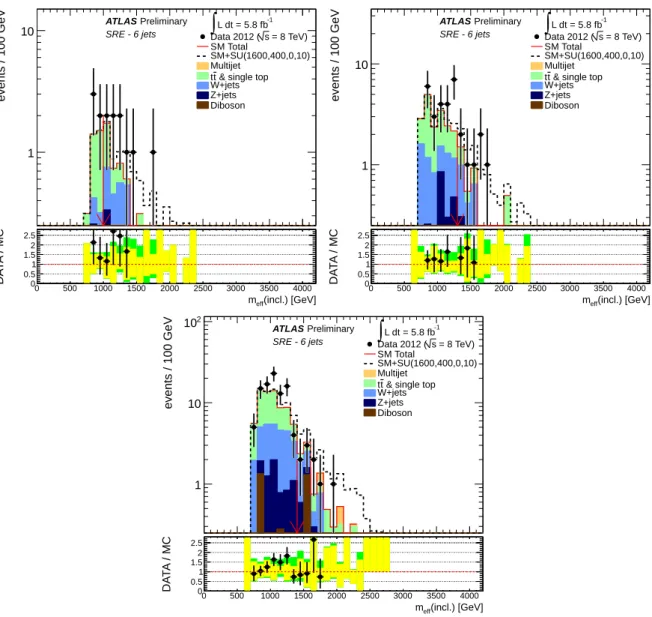
To estimate the backgrounds in a consistent and robust fashion, four control regions are defined for

each of the 12 signal regions, giving 48 CRs in total. The orthogonal CR event selections are designed to

CR SR background CR process CR selection

CRY Z(→νν)+jets γ+jets Isolated photon

CRQ QCD jets QCD jets Reversed∆φ(jet,E^miss_T )_minandE_T^miss/m_eff(N j) cuts

CRW W(→`ν)+jets W(→`ν)+jets 30 GeV<mT(`,E^miss_T )<100 GeV,b-veto

CRT tt¯and single-t tt¯→bbqq⁰`ν 30 GeV<mT(`,E^miss_T )<100 GeV,b-tag

Table 2: Control regions used in the analysis: the main targeted background in the SR, the process used to model the background, and main CR cut(s) used to select this process are given.

provide uncorrelated data samples enriched in particular background sources. Each ensemble of one SR and four CRs constitutes a different ‘stream’ of the analysis. The CR selections are optimised to maintain adequate statistical weight and low SUSY signal contamination, while minimising as far as possible the systematic uncertainties arising from the extrapolation to the SR.

The CRs are listed in Table 2. CRY is used to estimate the contribution of Z(

events to each SR by selecting a sample of

minimum angular separation in the transverse plane between up to three selected leading jets (depending on channel) and

(∆

)

in Table 1), together with a reversed cut on E

(N j), to produce data samples enriched in multi-jet background events. CRW and CRT use respectively a b- jet veto or b-jet requirement together with a lepton

E

transverse mass (m

) requirement to select samples of W(

t¯ t background events. Cross-checks are performed using several ‘validation region’ samples selected with requirements minimally correlated with those used in the CRs. For example, CRY estimates of the Z(→

jets background are validated with samples of Z(

the di-lepton invariant mass lies within 25 GeV of the mass of the Z boson.

5 Analysis procedure

The observed numbers of events in the CRs for each SR are used to generate internally consistent SM background estimates for the SR via a likelihood fit. This procedure enables CR correlations and con- tamination by other SM processes and

or SUSY signal events to be taken into account. The same fit also allows the statistical significance of the observation in the SR to be determined. Key ingredients in the fit are the ratios of expected event counts (the transfer factors TFs) from each background process between the SR and each CR, and between CRs. The TFs enable observations in the CRs to be converted into background estimates in the SR using:

N(SR, scaled)

N(CR, obs)

"

N(SR, unscaled)

N(CR, unscaled)

#

,

(1)

where N(SR, scaled) is the estimated background contribution to the SR by a given process, N(CR, obs) is the observed number of data events in the CR for the process, and N(SR, unscaled) and N(CR, unscaled) are a priori estimates of the contributions from the process to the SR and CR, respectively. The ratio appearing in the square brackets in Eqn. 1 is defined to be the transfer factor TF. Similar equations containing inter-CR TFs enable the background estimates to be normalised coherently across all the CRs.

Background estimation requires determination of the central expected values of the TFs for each SM process, together with their associated correlated and uncorrelated uncertainties. The multi-jet TFs are estimated using a data-driven technique [17], which applies a resolution function to well-measured multi- jet events in order to estimate the impact of jet energy mismeasurement and heavy-flavor semileptonic

miss

validated with data. Some systematic uncertainties, for instance those arising from the jet energy scale (JES), or theoretical uncertainties in MC cross sections, largely cancel when calculating the event count ratios constituting the TFs.

The result of the likelihood fit for each SR-CR ensemble is a set of background estimates and un- certainties for the SR together with a p-value giving the probability for the hypothesis that the SR event count is compatible with background alone. However, an assumption has to be made about the migration of signal events between regions. When searching for a signal in a particular SR, first it is assumed that the signal contributes only to the SR, i.e. the signal TFs are all set to zero, giving no contribution from the signal in the CRs. If no excess is observed, then limits are set within specific SUSY parameter spaces, taking into account the contribution of signal in the CRs and the theoretical and experimental uncertainties on the SUSY production cross section and kinematic distributions. Exclusion limits are obtained using a likelihood test. This compares the observed event rates in the signal regions with the fitted background expectation and expected signal contributions, for various signal hypotheses.

MC samples are used to develop the analysis, optimise the selections, determine the transfer factors used to estimate the W

jets, Z

jets, top quark and di-boson backgrounds, and to assess sensitivity to specific SUSY signal models. The following MC generators are used:

•

Samples of W events with accompanying jets are generated with SHERPA using the MENLOPS pre- scription [34, 35]. Theoretical uncertainties are evaluated by comparison with samples produced using ALPGEN [36] and the LO CTEQ6L1 [37] PDF set. Z/γ

and

events with accompanying jets are generated with ALPGEN.

•

Samples of top quark pair events with accompanying jets, assuming m

172.5 GeV, are gen- erated with MC@NLO [38, 39] and the Next-to-Leading Order (NLO) PDF set CT10 [40], which is used for all NLO MC. Theoretical uncertainties are evaluated by comparison with samples pro- duced using SHERPA [41].

•

Samples of single top quark events with accompanying jets are generated with MC@NLO for the s-channel and Wt processes and AcerMC [42] interfaced to PYTHIA6 using CTEQ6L1 PDF set for the t-channel process.

•

Samples of WW , WZ, ZZ, Wγ and Zγ events are generated with SHERPA.

Fragmentation and hadronisation for all ALPGEN and MC@NLO samples is performed with HERWIG, using JIMMY for the underlying event.

SUSY signal samples are generated with HERWIG++ [43] or MadGraph

PYTHIA [44–46]. Signal cross sections are calculated to next-to-leading order in the strong coupling constant, including the resumma- tion of soft gluon emission at next-to-leading-logarithmic accuracy (NLO

NLL) [47–51].

The MC samples are generated using the same parameter set as Refs. [53–55]. SM background sam- ples are passed through the ATLAS detector simulation [56] based on GEANT4 [57] while SUSY signal samples are passed through a fast simulation using a parameterisation of the performance of the ATLAS electromagnetic and hadronic calorimeters. Differing pile-up (multiple proton-proton interactions in a given event) conditions as a function of the LHC instantaneous luminosity are taken into account by over- laying simulated minimum-bias events onto the hard-scattering process and reweighting them according to the mean number of interactions expected.

6 Systematic Uncertainties

Systematic uncertainties arise through the use of the transfer factors relating observations in the control

regions to background expectations in the signal regions, and from the modelling of the SUSY signal. For

the MC-derived transfer factors the primary common sources of systematic uncertainty are the jet energy scale (JES) calibration, jet energy resolution (JER), MC modelling and the reconstruction performance in the presence of pile-up.

The JES uncertainty has been measured using the techniques described in Ref. [25, 28], with a slight dependence upon p

,

and proximity to adjacent jets. The JER uncertainty was estimated using the methods discussed in Ref. [58]. Contributions are added to both the JES and the JER uncertainties to account for the effect of pile-up at the relatively high luminosity delivered by the LHC in the 2012 run.

Modelling uncertainties arising from scale dependence and other theoretical e

ects are evaluated by comparing TFs obtained from samples generated with a variety of different MC generators, as described in Section 4. Additional uncertainties arising from photon and lepton reconstruction efficiency, energy scale and resolution (CRY, CRW and CRT), b-tag

veto e

ciency (CRW and CRT) and photon acceptance (CRY) are also considered. In CRW and CRT, an additional uncertainty is applied to the current ATLAS implementation of SHERPA W

tween SHERPA and other generators. Uncertainties on the multi-jet transfer factors are dominated by the modelling of the resolution function.

The modelling of SHERPA W

in ”loose” and ”medium” selections. For the ”tight” selections, the limited Monte Carlo statistics become also one of the major sources of uncertainty.

Initial state radiation (ISR) can significantly affect the signal visibility for SUSY models with small mass splittings. Systematic uncertainties arising from the treatment of ISR are studied by varying the value of

and the MadGraph

PYTHIA matching parameters. The uncertainties are found to be negligible for large sparticle masses (m

300 GeV) and mass splittings (∆ m

300 GeV), and to rise linearly with decreasing mass and decreasing mass splitting to

m

0 and m

300 GeV, and to

∆

m

0 and m

250 GeV.

7 Results, Interpretation and Limits

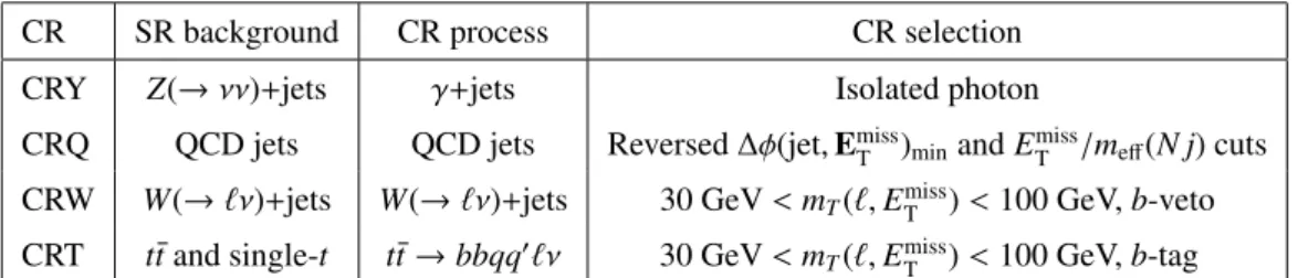
The number of events observed in the data and the number of SM events expected to enter each of the signal regions, determined using the likelihood fit, are shown in Table 3. Good agreement is ob- served between the data and the SM prediction, with no significant excess. Predictions obtained from the likelihood fits for the numbers of events in the validation regions also agree well with the observations.

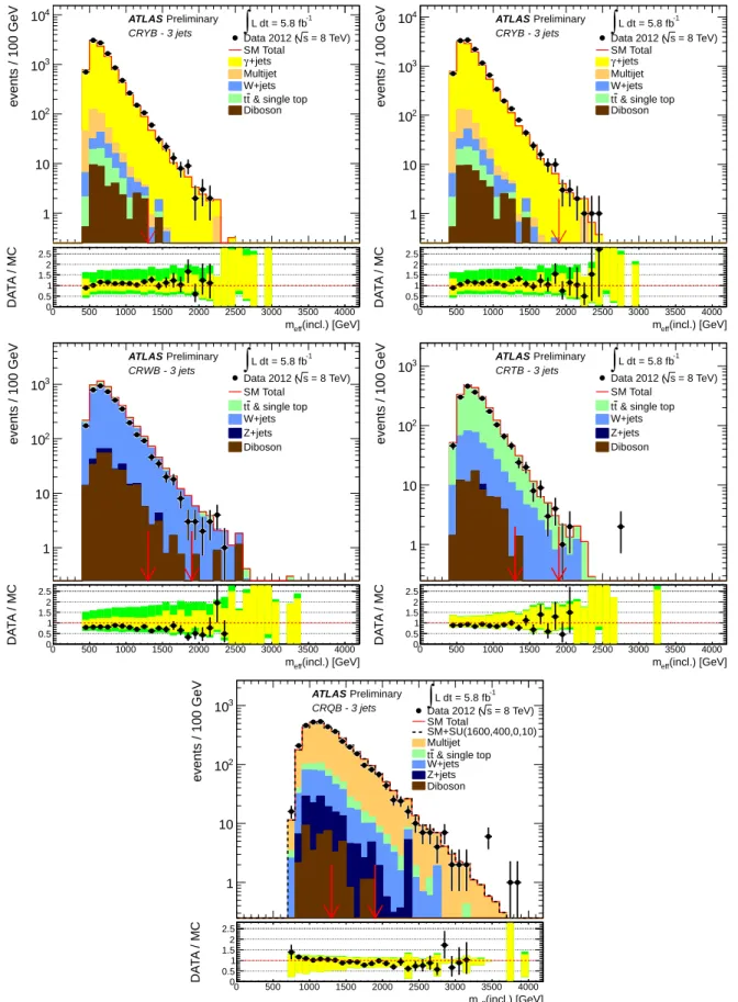
Distributions of m

(incl.) before the final cut on this quantity for data and the different MC samples nor-

malised with the theoretical cross sections are shown in Figures 1–5 for each of the channels. A typical

SUSY signal is shown for illustration. Equivalent distributions for the CRs can be found in Appendix A.

(incl.) [GeV]

meff

0 500 1000 1500 2000 2500 3000 3500 4000

events / 100 GeV

1 10 102

103

104

L dt = 5.8 fb-1

∫

Data 2012 ( SM Total

SM+SU(1600,400,0,10) Multijet

& single top t

tW+jets Z+jets Diboson Preliminary

ATLAS SRA - 2 jets

(incl.) [GeV]

meff

0 500 1000 1500 2000 2500 3000 3500 4000

DATA / MC

0 0.5 1 1.5 2 2.5

(incl.) [GeV]

meff

0 500 1000 1500 2000 2500 3000 3500 4000

events / 100 GeV

1 10 102

103

104

L dt = 5.8 fb-1

∫

Data 2012 ( SM Total

SM+SU(1600,400,0,10) Multijet

& single top t

tW+jets Z+jets Diboson Preliminary

ATLAS SRA - 2 jets

(incl.) [GeV]

meff

0 500 1000 1500 2000 2500 3000 3500 4000

DATA / MC

0 0.5 1 1.5 2 2.5

Figure 1: Observed m

(incl.) distributions for channel A for “loose” or “medium” (left) and “tight”

(right) cuts. The histograms denote the MC background expectations, normalised to cross section times integrated luminosity. In the lower panels the yellow error bands denote the experimental and MC statis- tical uncertainties, while the green bands show the total uncertainty. The red arrows indicate the values at which the cuts on m

(incl.) are applied. The expected distributions for a MSUGRA/CMSSM bench- mark model point with m

1600 GeV, m

400 GeV, A

0, tan

10 and

0 are also shown for comparison.

(incl.) [GeV]

meff

0 500 1000 1500 2000 2500 3000 3500 4000

events / 100 GeV

1 10 102

103

104 -1

L dt = 5.8 fb

∫

Data 2012 ( SM Total

SM+SU(1600,400,0,10) Multijet

& single top t

tW+jets Z+jets Diboson Preliminary

ATLAS SRB - 3 jets

(incl.) [GeV]

meff

0 500 1000 1500 2000 2500 3000 3500 4000

DATA / MC

0 0.5 1 1.5 2 2.5

(incl.) [GeV]

meff

0 500 1000 1500 2000 2500 3000 3500 4000

events / 100 GeV

1 10 102

103

104

∫

SM+SU(1600,400,0,10) Multijet

& single top t

tW+jets Z+jets Diboson Preliminary

ATLAS SRB - 3 jets

(incl.) [GeV]

meff

0 500 1000 1500 2000 2500 3000 3500 4000

DATA / MC

0 0.5 1 1.5 2 2.5

Figure 2: Observed m

(incl.) distributions for channel B for “medium” (left) and “tight” (right) cuts.

The histograms denote the MC background expectations, normalised to cross section times integrated

luminosity. In the lower panels the yellow error bands denote the experimental and MC statistical uncer-

tainties, while the green bands show the total uncertainty. The red arrows indicate the values at which the

cuts on m

(incl.) are applied. The expected distributions for a MSUGRA/CMSSM benchmark model

point with m

1600 GeV, m

400 GeV, A

0, tan

10 and

0 are also shown for comparison.

(incl.) [GeV]

meff

0 500 1000 1500 2000 2500 3000 3500 4000

events / 100 GeV

1 10 102

103

∫

SM+SU(1600,400,0,10) Multijet

& single top t

tW+jets Z+jets Diboson Preliminary

ATLAS SRC - 4 jets

(incl.) [GeV]

meff

0 500 1000 1500 2000 2500 3000 3500 4000

DATA / MC

0 0.5 1 1.5 2 2.5

(incl.) [GeV]

meff

0 500 1000 1500 2000 2500 3000 3500 4000

events / 100 GeV

1 10 102

103

L dt = 5.8 fb-1

∫

Data 2012 ( SM Total

SM+SU(1600,400,0,10) Multijet

& single top t

tW+jets Z+jets Diboson Preliminary

ATLAS SRC - 4 jets

(incl.) [GeV]

meff

0 500 1000 1500 2000 2500 3000 3500 4000

DATA / MC

0 0.5 1 1.5 2 2.5

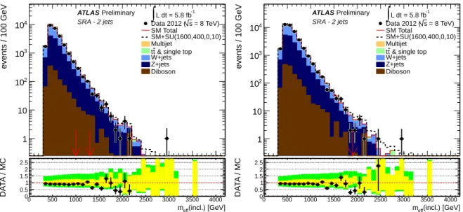
Figure 3: Observed m

(incl.) distributions for channel C for “loose” or “medium” (left) and “tight”

(right) cuts. The histograms denote the MC background expectations, normalised to cross section times integrated luminosity. In the lower panels the yellow error bands denote the experimental and MC statis- tical uncertainties, while the green bands show the total uncertainty. The red arrows indicate the values at which the cuts on m

(incl.) are applied. The expected distributions for a MSUGRA

CMSSM bench- mark model point with m

1600 GeV, m

400 GeV, A

0, tan

10 and

0 are also shown for comparison.

(incl.) [GeV]

meff

0 500 1000 1500 2000 2500 3000 3500 4000

events / 100 GeV

1 10 102

L dt = 5.8 fb-1

∫

Data 2012 ( SM Total

SM+SU(1600,400,0,10) Multijet

& single top t

tW+jets Z+jets Diboson Preliminary

ATLAS SRD - 5 jets

(incl.) [GeV]

meff

0 500 1000 1500 2000 2500 3000 3500 4000

DATA / MC

0 0.5 1 1.5 2 2.5

Figure 4: Observed m

(incl.) distribution for channel D. The histograms denote the MC background

expectations, normalised to cross section times integrated luminosity. In the lower panels the yellow

error bands denote the experimental and MC statistical uncertainties, while the green bands show the

total uncertainty. The red arrow indicate the value at which the cut on m

(incl.) is applied. The expected

distributions for a MSUGRA/CMSSM benchmark model point with m

m

A

0 are also shown for comparison.

(incl.) [GeV]

meff

0 500 1000 1500 2000 2500 3000 3500 4000

events / 100 GeV

1 10

L dt = 5.8 fb-1

∫

Data 2012 ( SM Total

SM+SU(1600,400,0,10) Multijet

& single top t

tW+jets Z+jets Diboson Preliminary

ATLAS SRE - 6 jets

(incl.) [GeV]

meff

0 500 1000 1500 2000 2500 3000 3500 4000

DATA / MC

0 0.5 1 1.5 2 2.5

(incl.) [GeV]

meff

0 500 1000 1500 2000 2500 3000 3500 4000

events / 100 GeV

1 10

L dt = 5.8 fb-1

∫

Data 2012 ( SM Total

SM+SU(1600,400,0,10) Multijet

& single top t

tW+jets Z+jets Diboson Preliminary

ATLAS SRE - 6 jets

(incl.) [GeV]

meff

0 500 1000 1500 2000 2500 3000 3500 4000

DATA / MC

0 0.5 1 1.5 2 2.5

(incl.) [GeV]

meff

0 500 1000 1500 2000 2500 3000 3500 4000

events / 100 GeV

1 10

102 -1

L dt = 5.8 fb

∫

Data 2012 ( SM Total

SM+SU(1600,400,0,10) Multijet

& single top t

tW+jets Z+jets Diboson Preliminary

ATLAS SRE - 6 jets

(incl.) [GeV]

meff

0 500 1000 1500 2000 2500 3000 3500 4000

DATA / MC

0 0.5 1 1.5 2 2.5

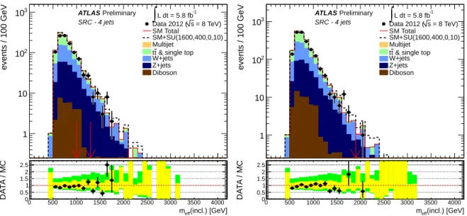
Figure 5: Observed m

(incl.) distributions for channel E for “loose” (top left), “medium” (top right) and

“tight” (bottom) cuts. The histograms denote the MC background expectations, normalised to cross sec-

tion times integrated luminosity. In the lower panels the yellow error bands denote the experimental and

MC statistical uncertainties, while the green bands show the total uncertainty. The red arrows indicate the

values at which the cuts on m

(incl.) are applied. The expected distributions for a MSUGRA/CMSSM

benchmark model point with m

m

A

0 are also shown

for comparison.

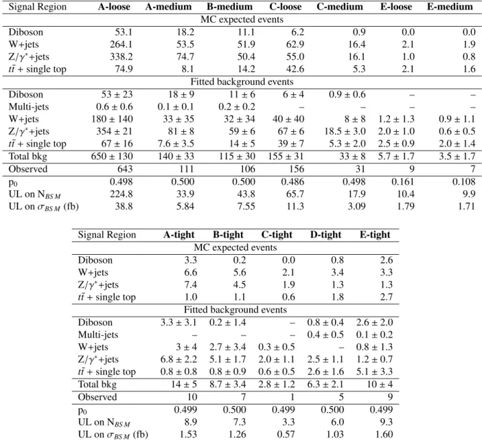
Signal Region A-loose A-medium B-medium C-loose C-medium E-loose E-medium MC expected events

Diboson 53.1 18.2 11.1 6.2 0.9 0.0 0.0

W+jets 264.1 53.5 51.9 62.9 16.4 2.1 1.9

Z/γ^∗+jets 338.2 74.7 50.4 55.0 16.1 1.0 0.8

tt¯+single top 74.9 8.1 14.2 42.6 5.3 2.1 1.6

Fitted background events

Diboson 53±23 18±9 11±6 6±4 0.9±0.6 – –

Multi-jets 0.6±0.6 0.1±0.1 0.2±0.2 – – – –

W+jets 180±140 33±35 32±34 40±40 8±8 1.2±1.3 0.9±1.1 Z/γ^∗+jets 354±21 81±8 59±6 67±6 18.5±3.0 2.0±1.0 0.6±0.5 tt¯+single top 67±16 7.6±3.5 14±5 39±7 5.3±2.0 2.5±0.9 2.0±1.4 Total bkg 650±130 140±33 115±30 155±31 33±8 5.7±1.7 3.5±1.7

Observed 643 111 106 156 31 9 7

p₀ 0.498 0.500 0.500 0.486 0.498 0.161 0.108

UL on N_{BS M} 224.8 33.9 43.8 65.7 17.9 10.4 9.9

UL onσ_{BS M}(fb) 38.8 5.84 7.55 11.3 3.09 1.79 1.71

Signal Region A-tight B-tight C-tight D-tight E-tight MC expected events

Diboson 3.3 0.2 0.0 0.8 2.6

W+jets 6.6 5.6 2.1 3.4 3.3

Z/γ^∗+jets 7.4 4.5 1.9 1.3 1.3

tt¯+single top 1.0 1.1 0.6 1.8 2.7

Fitted background events

Diboson 3.3±3.1 0.2±1.4 – 0.8±0.4 2.6±2.0

Multi-jets – – – 0.4±0.5 0.1±0.2

W+jets 3±4 2.7±3.4 0.3±0.5 – 0.8±1.3 Z/γ^∗+jets 6.8±2.2 5.1±1.7 2.0±1.1 2.5±1.1 1.2±0.7 t¯t+single top 0.8±0.8 0.8±0.9 0.6±0.5 2.6±1.6 5.1±3.3 Total bkg 14±5 8.7±3.4 2.8±1.2 6.3±2.1 10±4

Observed 10 7 1 5 9

p0 0.499 0.500 0.499 0.500 0.499

UL on NBS M 8.9 7.3 3.3 6.0 9.3

UL onσBS M (fb) 1.53 1.26 0.57 1.03 1.60

Table 3: Numbers of events observed in the signal regions used in the analysis compared with background

expectations obtained from the fits described in the text. No signal contribution is considered in the CRs

for the fit. Empty cells correspond to estimates lower than 0.01. The p-values give the probabilities of

the observations being consistent with the estimated backgrounds. During their computation, p-values

are bounded to 0.5. The last two lines show the 95% CL upper limits (UL) on the excess number of

events and cross sections above those expected from the Standard Model.

[GeV]

m0

500 1000 1500 2000 2500 3000 3500

[GeV]1/2m

300 350 400 450 500 550 600 650 700 750 800

(1000 GeV) q~

(1400 GeV) q ~

(1800 GeV) q ~

(1000 GeV) g~

(1200 GeV) g~ (1400 GeV) g~ (1600 GeV) g~

>0 µ

= 0, = 10, A0

β MSUGRA/CMSSM: tan

=8 TeV s

-1, L dt = 5.8 fb

∫

0-lepton combined

ATLAS

theory) σSUSY

±1 Observed limit (

exp) σ

±1 Expected limit (

, 7 TeV) Observed limit (4.7 fb-1 Non-convergent RGE No EW-SB Preliminary

gluino mass [GeV]

200 400 600 800 1000 1200 1400 1600 1800

squark mass [GeV]

500 1000 1500 2000 2500 3000

<0µ = 5, βCDF, Run II, tan <0µ = 3, βD0, Run II, tan

>0 µ

= 0, = 10, A0

β MSUGRA/CMSSM: tan

=8 TeV s

-1, L dt = 5.8 fb

∫

0-lepton combined

ATLAS

theory) σSUSY

±1 Observed limit (

exp) σ

±1 Expected limit ( Theoretically excluded Stau LSP Preliminary

Figure 6: 95% CL exclusion limits for MSUGRA

CMSSM models with tan

10, A

0 and

0 presented (left) in the m

–m

plane and (right) in the m

–m

plane. Exclusion limits are obtained by using the signal region with the best expected sensitivity at each point. The blue dashed lines show the expected limits at 95% CL, with the light (yellow) bands indicating the 1σ excursions due to experimen- tal uncertainties. Observed limits are indicated by medium (maroon) curves, where the solid contour represents the nominal limit, and the dotted lines are obtained by varying the cross section by the the- oretical scale and PDF uncertainties. Previous results from ATLAS [17] are represented by the shaded (light blue) area. The theoretically excluded regions (green and blue) are described in Ref. [63].

Data from all the channels are used to set limits on SUSY models, taking the SR with the best expected sensitivity at each point in several parameter spaces. A profile log-likelihood ratio test in com- bination with the CL

prescription [59] is used to derive 95% CL exclusion regions. Exclusion limits are obtained by using the signal region with the best expected sensitivity at each point. The nominal signal cross section and the uncertainty are taken from an ensemble of cross section predictions using different PDF sets and factorisation and renormalisation scales, as described in Ref. [52]. Observed limits are calculated for both the nominal cross section, and

uncertainties. For each of these three individual limits, the best signal region at each point is taken. Numbers quoted in the text are evaluated from the observed exclusion limit based on the nominal cross section less one sigma on the theoretical uncertainty.

In Fig. 6 the results are interpreted in the tan

10, A

0,

0 slice of MSUGRA

CMSSM models

2

. For the nominal cross sections, the best signal region is E-tight for high m

values, C-tight for low m

values and D-tight between the two. Results are presented in both the m

–m

and m

–m

planes. The sparticle mass spectra and decay tables are calculated with SUSY-HIT [60] interfaced to SOFTSUSY [61]

and SDECAY [62].

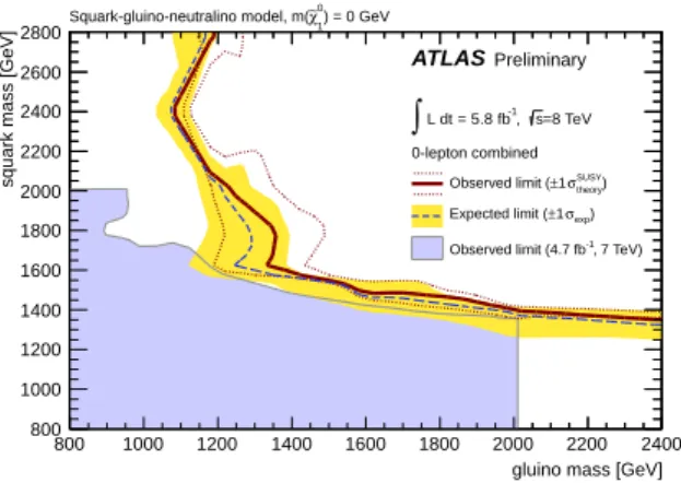
An interpretation of the results is presented in Figure 7 as a 95% CL exclusion region in the (m

m

)- plane for a simplified set of SUSY models with m

1 =

0. In these models the gluino mass and the masses of the squarks of the first two generations are set to the values shown on the axes of the figure. All other supersymmetric particles, including the squarks of the third generation, are decoupled.

In Fig. 8 limits are shown for three classes of simplified model in which only direct production of (a) gluino pairs, (b) ‘light’-flavor squarks (of the first two generations) and gluinos or (c) light-flavor squark pairs is kinematically possible, with all other superpartners, except for the neutralino LSP, decoupled.

This forces each light-flavor squark or gluino to decay directly to jets and an LSP. Cross sections are evaluated assuming decoupled light-flavor squarks or gluinos in cases (a) and (c), respectively. In all cases squarks of the third generation are decoupled. In case (b) the masses of the light-flavor squarks are

2Five parameters are needed to specify a particular MSUGRA/CMSSM model: the universal scalar mass,m0, the universal gaugino massm1/2, the universal trilinear scalar coupling,A0, the ratio of the vacuum expectation values of the two Higgs fields, tanβ, and the sign of the higgsino mass parameter,µ=±.

gluino mass [GeV]

800 1000 1200 1400 1600 1800 2000 2200 2400

squark mass [GeV]

800 1000 1200 1400 1600 1800 2000 2200 2400 2600

2800 ^{) = 0 GeV}

0

χ∼1

Squark-gluino-neutralino model, m(

=8 TeV s

-1, L dt = 5.8 fb

∫

0-lepton combined

ATLAS

theory) σSUSY

±1 Observed limit (

exp) σ

±1 Expected limit (

, 7 TeV) Observed limit (4.7 fb-1

Preliminary

Figure 7: A simplified MSSM scenario with only strong production of gluinos and first- and second- generation squarks, with direct decays to jets and neutralinos. Exclusion limits are obtained by using the signal region with the best expected sensitivity at each point. The blue dashed lines show the expected limits at 95% CL, with the light (yellow) bands indicating the 1σ experimental uncertainties. Observed limits are indicated by medium (maroon) curves, where the solid contour represents the nominal limit, and the dotted lines are obtained by varying the cross section by the theoretical scale and PDF uncertain- ties. Previous results from ATLAS [17] are represented by the shaded (light blue) area. Results at 7 TeV are valid for squark or gluino masses below 2000 GeV, the mass range studied for that analysis.

set to 0.96 times the mass of the gluino.

In the CMSSM

MSUGRA case, the limit on m

is above 340 GeV at high m

and reaches 710 GeV for low values of m

. Equal mass light-flavor squarks and gluinos are excluded below 1500 GeV in this scenario. The same limit of 1500 GeV for equal mass of light-flavor squarks and gluinos is found for the simplified MSSM scenario shown in Fig. 7. In the simplified model cases of Fig. 8 (a) and (c), when the lightest neutralino is massless the limit on the gluino mass (case (a)) is 1100 GeV, and that on the light-flavor squark mass (case (c)) is 630 GeV. Mass limits for the direct production of light- flavor squarks (case (c)) hardly improve with respect to the 7 TeV data analysis because of increased background predictions and uncertainties at 8 TeV in the low m

and low jet multiplicity channels used to provide exclusions for these models.

8 Summary

This note reports a search for new physics in final states containing high-p

jets, missing transverse momentum and no electrons or muons, based on a 5.8 fb

dataset recorded by the ATLAS experiment at the LHC in 2012. Good agreement is seen between the numbers of events observed in the data and the numbers of events expected from SM processes.

The results are interpreted both in terms of MSUGRA/CMSSM models with tan

10, A

0 and

0, and in terms of simplified models with only light-flavor squarks, or gluinos, or both, together

with a neutralino LSP, with the other SUSY particles decoupled. In the MSUGRA/CMSSM models,

values of m

350 GeV are excluded at the 95% confidence level for all values of m

, and m

740

GeV for low m

. Equal mass squarks and gluinos are excluded below 1500 GeV in this scenario. When

the neutralino is massless, gluino masses below 1100 GeV are excluded at the 95% confidence level in

a simplified model with only gluinos and the lightest neutralino. For a simplified model involving the

strong production of squarks of the first two generations, with decays to a massless neutralino, squark

masses below 630 GeV are excluded.

[GeV]

g~

m

200 400 600 800 1000 1200 1400

[GeV]0 1χ∼m

200 400 600 800 1000 1200 1400

0

χ∼1

q q

→ g~ production;

~g g~

=8 TeV s

-1, L dt = 5.8 fb

∫

0-lepton combined

Preliminary

ATLAS Observed limit (±1 σ_theory^SUSY) exp) σ

±1 Expected limit (

, 7 TeV) Observed limit (4.7 fb-1

[GeV]

g~

m

200 400 600 800 1000 1200 1400

[GeV]0 1χ∼m

200 400 600 800 1000 1200 1400

0

χ∼1

q q

→

~g

0, χ∼1

→ q q~ production;

g~ q~

~g

=0.96m

q~

m

=8 TeV s

-1, L dt = 5.8 fb

∫

0-lepton combined

Preliminary ATLAS

theory) σSUSY

±1 Observed limit (

exp) σ

±1 Expected limit (

[GeV]

q~

m 200 300 400 500 600 700 800 900 1000 1100 1200 [GeV]0 1χ∼m

200 400 600 800 1000 1200

0

χ∼1

→ q q~ production;

q~ q~

=8 TeV s

-1, L dt = 5.8 fb

∫

0-lepton combined

Preliminary

ATLAS ₎

theory σSUSY

±1 Observed limit (

exp) σ

±1 Expected limit (

, 7 TeV) Observed limit (4.7 fb-1

Figure 8: Exclusion limits at 95% CL for direct production of (case a – top left) gluino pairs with

decoupled squarks, (case b – top right) light-flavor squarks and gluinos and (case c – bottom) light-

flavor squark pairs with decoupled gluinos. Gluinos (light-flavor squarks) are required to decay to two

(one) jet(s) and a neutralino LSP. Exclusion limits are obtained by using the signal region with the best

expected sensitivity at each point. The blue dashed lines show the expected limits at 95% CL, with the

light (yellow) bands indicating the 1σ excursions due to experimental uncertainties. Observed limits

are indicated by medium (maroon) curves, where the solid contour represents the nominal limit, and the

dotted lines are obtained by varying the cross section by the theoretical scale and PDF uncertainties.

References

[1] L. Evans and P. Bryant, LHC Machine, JINST

(2008) S08001.

[2] H. Miyazawa, Baryon Number Changing Currents, Prog. Theor. Phys.

(1966) 1266–1276.

[3] P. Ramond, Dual Theory for Free Fermions, Phys. Rev.

(1971) 2415–2418.

[4] Y. A. Golfand and E. P. Likhtman, Extension of the Algebra of Poincare Group Generators and Violation of p Invariance, JETP Lett.

(1971) 323–326. [Pisma Zh. Eksp. Teor. Fiz. 13 (1971) 452-455].

[5] A. Neveu and J. H. Schwarz, Factorizable dual model of pions, Nucl. Phys.

(1971) 86–112.

[6] A. Neveu and J. H. Schwarz, Quark Model of Dual Pions, Phys. Rev.

(1971) 1109–1111.

[7] J. Gervais and B. Sakita, Field theory interpretation of supergauges in dual models, Nucl. Phys.

B34

(1971) 632–639.

[8] D. V. Volkov and V. P. Akulov, Is the Neutrino a Goldstone Particle?, Phys. Lett.

(1973) 109–110.

[9] J. Wess and B. Zumino, A Lagrangian Model Invariant Under Supergauge Transformations, Phys.

Lett.

(1974) 52.

[10] J. Wess and B. Zumino, Supergauge Transformations in Four-Dimensions, Nucl. Phys.

(1974) 39–50.

[11] P. Fayet, Supersymmetry and Weak, Electromagnetic and Strong Interactions, Phys. Lett.

(1976) 159.

[12] P. Fayet, Spontaneously Broken Supersymmetric Theories of Weak, Electromagnetic and Strong Interactions, Phys. Lett.

(1977) 489.

[13] G. R. Farrar and P. Fayet, Phenomenology of the Production, Decay, and Detection of New Hadronic States Associated with Supersymmetry, Phys. Lett.

(1978) 575–579.

[14] P. Fayet, Relations Between the Masses of the Superpartners of Leptons and Quarks, the Goldstino Couplings and the Neutral Currents, Phys. Lett.

(1979) 416.

[15] S. Dimopoulos and H. Georgi, Softly Broken Supersymmetry and SU(5), Nucl. Phys.

(1981) 150.

[16] ATLAS Collaboration, Search for supersymmetry in final states with jets, missing transverse momentum and one isolated lepton in

s

7 TeV pp collisions using 1 f b

of ATLAS data, Phys.

Rev.

(2012) 012006, arXiv:1109.6606 [hep-ex].

[17] ATLAS Collaboration, Search for squarks and gluinos with the ATLAS detector in final states with jets and missing transverse momentum using 4.7 fb

of

s

7 TeV proton-proton collision data, arXiv:1208.0949 [hep-ex].

[18] ATLAS Collaboration, Search for squarks and gluinos with the ATLAS detector using final states with jets and missing transverse momentum and 4.7 fb

of

s

7 TeV proton-proton collision

data, ATLAS-CONF-2012-033, http://cdsweb.cern.ch/record/1432199.

[19] ATLAS Collaboration, Search for squarks and gluinos using final states with jets and missing transverse momentum with the ATLAS detector in sqrt(s)

7 TeV proton-proton collisions, Phys.

Lett.

(2012) 67–85, arXiv:1109.6572 [hep-ex].

[20] ATLAS Collaboration, Search for squarks and gluinos using final states with jets and missing transverse momentum with the ATLAS detector in

s

7 TeV proton-proton collisions, ATLAS-CONF-2011-086, http://cdsweb.cern.ch/record/1356194.

[21] ATLAS Collaboration, Search for squarks and gluinos using final states with jets and missing transverse momentum with the ATLAS detector in sqrt(s)

7 TeV proton-proton collisions, Phys.Lett.

(2011) 186–203, arXiv:1102.5290 [hep-ex].

[22] ATLAS Collaboration, The ATLAS Experiment at the CERN Large Hadron Collider, 2008. JINST

(2008) S08003.

[23] M. Cacciari, G. P. Salam, and G. Soyez, The anti-k

jet clustering algorithm, JHEP

(2008) 063, arXiv:0802.1189 [hep-ph].

[24] M. Cacciari and G. P. Salam, Dispelling the N

myth for the k

jet-finder, Phys. Lett.

(2006) 57–61, arXiv:hep-ph/0512210.

[25] ATLAS Collaboration, Jet energy measurement with the ATLAS detector in proton-proton collisions at sqrt(s)

7 TeV, arXiv:1112.6426 [hep-ex].

[26] W. Lampl et al., Calorimeter Clustering Algorithms: Description and Performance, ATL-LARG-PUB-2008-002. http://cdsweb.cern.ch/record/1099735.

[27] ATLAS Collaboration, Expected Performance of the ATLAS Experiment - Detector, Trigger and Physics, CERN-OPEN-2008-020. arXiv:0901.0512 [hep-ex].

[28] ATLAS Collaboration, Single hadron response measurement and calorimeter jet energy scale uncertainty with the ATLAS detector at the LHC, arXiv:1203.1302 [hep-ex].

[29] ATLAS Collaboration, Electron performance measurements with the ATLAS detector using the 2010 LHC proton-proton collision data, Eur. Phys. J.

(2012) 1909, arXiv:1110.3174 [hep-ex].

[30] ATLAS Collaboration, Muon Momentum Resolution in First Pass Reconstruction of pp Collision Data Recorded by ATLAS in 2010, ATLAS-CONF-2011-046.

http://cdsweb.cern.ch/record/1338575.

[31] ATLAS Collaboration, Muon reconstruction e

ciency in reprocessed 2010 LHC proton-proton collision data recorded with the ATLAS detector, ATLAS-CONF-2011-063.

http://cdsweb.cern.ch/record/1345743.

[32] ATLAS Collaboration, Performance of Missing Transverse Momentum Reconstruction in

Proton-Proton Collisions at 7 TeV with ATLAS, Eur.Phys.J.

(2012) 1844, arXiv:1108.5602 [hep-ex].

[33] Selection of jets produced in proton-proton collisions with the ATLAS detector using 2011 data, ATLAS-CONF-2012-020. http://cdsweb.cern.ch/record/1430034.

[34] K. Hamilton and P. Nason, Improving NLO-parton shower matched simulations with higher order

matrix elements, JHEP

(2010) 039, arXiv:1004.1764 [hep-ph].