ATLAS-CONF-2014-016 01April2014
ATLAS NOTE
ATLAS-CONF-2014-016
April 1, 2014
Search for microscopic black holes and string balls in final states with leptons and jets with the ATLAS detector at √
s = 8 TeV
The ATLAS Collaboration
Abstract
A search for an excess of events with multiple high transverse momentum objects in- cluding charged leptons and jets is presented, using 20.3 fb−1 of proton-proton collision data recorded by the ATLAS detector at the Large Hadron Collider in 2012 at a centre-of- mass energy of √
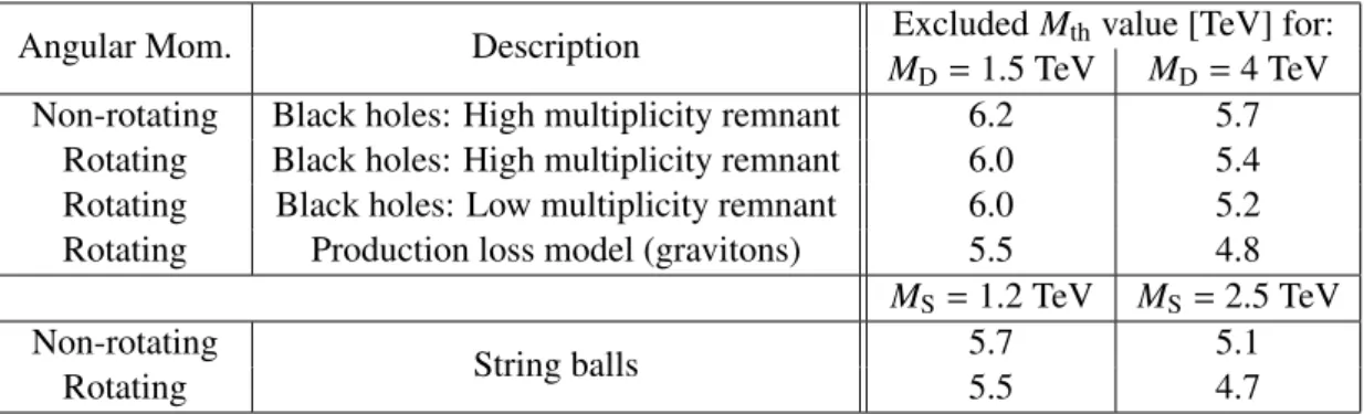
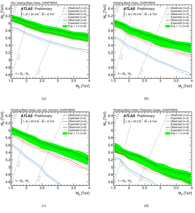
s = 8 TeV. No excess of events beyond Standard Model expectations is observed. Using extra-dimensional models for black hole and string ball production and decay, exclusion contours are determined as a function of the mass threshold for produc- tion and the fundamental gravity scale for two, four and six extra dimensions. For six extra dimensions, mass thresholds of 4.8 – 6.2 TeV are excluded at 95% confidence level, depend- ing on the fundamental gravity scale and model assumptions. Upper limits on the fiducial cross-sections for non-Standard Model production of these final states are set.
c
Copyright 2014 CERN for the benefit of the ATLAS Collaboration.
Reproduction of this article or parts of it is allowed as specified in the CC-BY-3.0 license.
1 Introduction
A long-standing problem in particle physics is the very large di
fference between two apparently funda- mental energy scales: the electroweak scale at
O(0.1 TeV) and the gravitational (Planck) scale M
Pl = O(1016TeV). Models postulating extra spatial dimensions into which the gravitational field propagates attempt to address this hierarchy problem [1–4]. Usually, the Standard Model (SM) fields are constrained to the three spatial and one time dimensions of our universe, whilst the gravitons also propagate into the n “bulk” extra dimensions. In these models, the fundamental gravitational scale in the full (n
+4) space- time dimensions, M
D, is dramatically lower than M
Pl, and represents an e
ffective scale appropriate for probes of the gravitational interactions at low energies. A value of M
Din the TeV range allows for the production of strong gravitational states such as microscopic black holes at energies accessible at the Large Hadron Collider (LHC) [5–7]. Two well motivated extra-dimensional models are those with large flat extra dimensions (ADD models [2, 3]) and those with small, usually warped, extra dimensions (RS models [4]). This analysis considers ADD models, for which the n
=1 case is strongly disfavoured by astrophysical and tabletop experiments [8]. Thus, benchmark models with two, four and six additional spatial dimensions are considered.
Estimates of black hole cross-sections invoke semi-classical approximations, the validity of which requires the production centre-of-mass energy to be significantly above M
D. This motivates the introduc- tion of a production mass threshold M
th, well above M
D. In the black hole formation stage, some energy is expected to be lost to gravitational or SM radiation. This has recently been calculated using numerical general relativity simulations [9].
Once a black hole has formed and settled into a Schwarzschild [10] (non-rotating) or Myers-Perry [11]
(rotating) state, it is assumed to lose mass and angular momentum through the emission of Hawking ra- diation [12]. All types of SM particles are emitted, although the graviton emission spectra have been calculated only for the non-rotating case [13, 14]. The emission energy spectrum is characterised by the Hawking temperature, which depends on n, and is larger for lower mass and for more highly ro- tating black holes. It is not a pure black-body spectrum, being modified by gravitational transmission coe
fficients (“grey-body factors") [15–20]. These encode the probability of transmission through the gravitational field of the black hole, and act primarily to disfavour low energy emissions. The relative particle emissivities depend on n, the black hole angular momentum and temperature, and the spin of the emitted particle. In the rotating case, the fluxes for vector emission are enhanced several-fold, due to the effect of super-radiance [17, 20]. Emissions reducing the angular momentum of the black hole are kinematically favoured. As the black hole evolves, its mass decreases, and, upon approaching M
D, quantum gravitational e
ffects become important and evaporation by emission of Hawking radiation is no longer a suitable model. This is the “remnant phase", in which the theoretical modelling uncertainties are large. The conventional treatment by the event generators used in LHC simulations is to decay the black hole remnant to a small number of SM particles [21].
Strong gravitational states include, in the context of weakly-coupled string theory, highly excited string states (string balls) [22]
1. In these models, the string scale M
Sand string coupling
gSdefine M
D = g−2/(nS +2)M
Sand determine the string ball properties. Black hole production and evaporation proceeds as described above, except that black holes evolve into highly excited string states once their mass drops below the correspondence point of
∼M
S/g2S. Thereafter, the string states continue to emit radiation, with a modified characteristic temperature.
The experimental signature of black hole decays is an ensemble of high-energy particles, the com- position of which varies both with model assumptions and M
D; for example, a rotating state leads to fewer emissions of more highly energetic particles. However, the universality of the gravitational cou- pling implies that particles are produced primarily according to the SM degrees of freedom (modified by
1Hereinafter all references to black holes also apply to string balls, unless otherwise stated.
the relative emissivities). This leads to a branching fraction to final states with at least one lepton
2of
∼
15
−50%, where the range is primarily a consequence of varying average multiplicities of the decay for different models and values of the parameters M
Dand M
th. The most significant uncertainties in the theoretical modelling of these states, which motivate exploration through benchmark models, arise from possible losses in the production phase, the lack of a description of graviton emission in the rotating case, and the treatment of the black hole remnant state near M
D. The latter can strongly impact the multiplicity of particles from black hole decays.
This note describes a search for an excess of events over SM expectations in 20.3 fb
−1of ATLAS pp collision data collected at
√s
=8 TeV in 2012. The analysis considers events at high
Pp
T, defined as the scalar sum of the p
Tof the selected reconstructed objects (hadronic jets and leptons), containing at least three high- p
Tobjects (leptons or jets), at least one of which must be a lepton. It is similar to a previous search [23], using
√s
=7 TeV data, which excluded at 95% confidence level (CL) black holes with M
th <4.5 TeV for M
D =1.5 TeV and n
=6. Greater sensitivity in this analysis comes from the higher centre-of-mass energy, larger integrated luminosity, as well as from the use of fits to improve background estimates at very high values of
Pp
T. Searches for black holes at
√s
=8 TeV have also been performed in like-sign di-muonic final states [24], as well as predominantly multi-jet final states [25]. The limits set, at 95% CL, for M
D=1.5 TeV and n
=6 are M
th >5.5 TeV and M
th >6.2 TeV, respectively. Corresponding limits for M
D=4 TeV and n
=6 are M
th >4.5 TeV and M
th >5.6 TeV.
Two-body final states have also been analysed elsewhere [26–28], with sensitivity to so-called quantum black holes, where the mass is close to M
D.
2 The ATLAS Detector
ATLAS [29] is a multipurpose detector with a forward-backward symmetric cylindrical geometry and nearly 4π coverage in solid angle
3. Closest to the beamline, the inner detector (ID) utilises fine-granularity pixel and microstrip detectors designed to provide precision track impact parameter and secondary ver- tex measurements. These silicon-based detectors cover the pseudorapidity range
|η| <2.5. A gas-filled straw-tube transition radiation tracking detector complements the silicon tracker at larger radii. The tracking detectors are immersed in a 2 T magnetic field produced by a thin superconducting solenoid lo- cated in the same cryostat as the barrel electromagnetic (EM) calorimeter. The EM calorimeters employ lead absorbers and use liquid argon as the active medium. The barrel EM calorimeter covers
|η| <1.5 and the end-cap EM calorimeters cover 1.4
< |η| <3.2. Hadronic calorimetry in the region
|η| <1.7 is achieved using steel absorbers and scintillating tiles as the active medium. Liquid argon calorimetry with copper absorbers is used in the hadronic end-cap calorimeters, which cover the region 1.5
< |η| <3.2.
The forward calorimeter (3.1
< η <4.9) uses copper and tungsten as the absorber with liquid argon as the active material. The muon spectrometer (MS) measures the deflection of muon tracks within
|η| <2.7, using three stations of precision drift tubes (with cathode strip chambers for the innermost station for
|η| >
2.0) located in a toroidal magnetic field of approximately 0.5 T and 1 T in the central and end- cap regions of ATLAS, respectively. The muon spectrometer is also instrumented with separate trigger chambers covering
|η|<2.4. A three-level trigger is used by the ATLAS detector. The first-level trigger is implemented in custom electronics, using a subset of detector information to reduce the event rate to a design value of 75 kHz. The second and third levels use software algorithms to yield a recorded event rate of about 400 Hz.
2Throughout this note, “lepton" denotes electrons and muons only.
3ATLAS uses a right-handed coordinate system with its origin at the nominal interaction point in the centre of the detector and thez-axis along the beam pipe. The x-axis points towards the centre of the LHC, and they-axis upwards. Cylindrical coordinates (r, φ) are used in the transverse plane,φbeing the azimuthal angle around the beam pipe. The pseudorapidityηis defined in terms of the polar angleθbyη=−ln tan(θ/2).
3 Trigger and Data Selection
The data used in this analysis were recorded in 2012, while the LHC was operating at a centre-of-mass energy of 8 TeV. The integrated luminosity was
RL
dt
=20.3 fb
−1. The uncertainty on the integrated luminosity is
±2.8%. It is derived, from a preliminary calibration of the luminosity scale derived frombeam-separation scans performed in November 2012, following the same methodology as that detailed in Ref. [30]. Events recorded by single electron and muon triggers under stable beam conditions and for which all detector subsystems were operational are considered. Single lepton triggers with different minimum p
Tthresholds are combined to increase the overall e
fficiency. The thresholds are 24 and 60 GeV for electron triggers and 24 and 36 GeV for muon triggers. The lower threshold triggers include isolation requirements on the candidate leptons, resulting in inefficiencies at higher p
Tthat are recovered by the triggers with higher p
Tthresholds. The trigger isolation criteria are looser than the requirements placed on the final reconstructed leptons. Events are required to have a reconstructed primary vertex with at least five associated tracks with p
T >0.4 GeV. In events with multiple reconstructed vertices the one with the largest sum of the squared p
Tof the tracks is taken as the primary interaction vertex.
4 Monte Carlo Simulation
Monte Carlo (MC) simulated events are used to help determine SM backgrounds and signal yields in the analysis. Background MC samples are processed through a detector simulation [31] based on GEANT4 [32] or a fast simulation using a parametrised response of the showers in the electromagnetic and hadronic calorimeters [31]. Additional scale factors are applied to bring the simulation into better agreement with the 2012 dataset. These include factors for lepton trigger, reconstruction and identifica- tion efficiencies.
Samples of W and Z/γ
∗4Monte Carlo events with accompanying jets are produced with S
herpa1.4.1 [33], using the CT10 [34] set of parton distribution functions (PDF). Events generated with A
lpgen2.14 [35]
use the CTEQ6L1 [36] PDF set and are interfaced to Pythia 6.426 [37] for parton showers and hadronisa- tion with the P
erugia2011C tune; these are used to assess modelling uncertainties. The cross-section nor- malisations are set to the inclusive next-to-next-to-leading order (NNLO) prediction from the DYNNLO program [38].
The production of top quark pairs is simulated with POWHEG r2129 [39] for the matrix element using the CT10 PDF set, with the top quark mass set to 172.5 GeV. Parton showering and hadronisation are performed with Pythia 6.426 with the Perugia2011C tune. Modelling uncertainties are assessed using events events generated with A
lpgen2.14 [35], using the CTEQ6L1 [36] PDF set and interfaced to H
erwig6.5.20 [40] for parton showers and hadronisation. The t¯ t cross-section is normalised to 253
+−1513pb, calculated at NNLO in QCD including resummation of next-to-next-to-leading logarithmic (NNLL) soft gluon terms with Top++ 2.0 [41–46].
Single top samples corresponding to three production modes: s-channel, t-channel and Wt-channel, are generated separately. For the s- and Wt-channel, events are generated with MC@NLO 4.06 [47], interfaced to Herwig++ 2.6.3 [48] for parton showering and hadronisation. The t-channel events are generated with A
cerMC 3.8 [49] interfaced to P
ythia6.426. For all three channels, the CT10 PDF set is used with the AUET2B [50] tune, and events are reweighted using the NNLO
+NNLL cross-sections as given in Refs. [51–53]. Di-boson (WW , WZ, ZZ) production is simulated with Herwig 6.5.20 using the CTEQ6L1 PDF set and the AU2 tune [54], normalised to the NLO prediction of MCFM 6.2 [55, 56].
The canonical Monte Carlo generators for the production of black hole signals are C
harybdis2.104 [57]
and Blackmax 2.2.0 [58, 59]. Both programs are able to simulate a range of rotating and non-rotating black hole and string ball states, exploring the theoretical modelling uncertainties discussed in Section 1.
4Hereinafter, all mention ofZ+jets refers to theZ/γ∗+jets process.
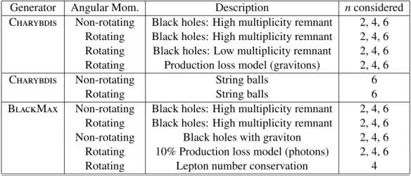
A variety of benchmark models simulated with both generators are used to illustrate possible black hole models. They are described in detail below and summarised in Table 1. The shower evolution and hadro- nisation of all signal samples uses Pythia 8.165 [60], with the MSTW2008lo [61] PDF set and the AU2 tune. The black hole mass is set as the QCD scale. The detector response is simulated using the ATLAS fast simulation. The benchmark grids are generated for two, four and six extra dimensions.
Both Monte Carlo generators are able to include the effects of the black hole angular momentum, with similar treatments of the Hawking evaporation. In contrast, they contain complementary and differ- ent modelling options for the more uncertain decay phases. Both generators model losses of mass and angular momentum in the production phase: Charybdis uses a model based on the Yoshino-Rychkov bounds [57, 62], favouring smaller losses of mass and angular momentum in the form of gravitons, whereas B
lackmaxparametrises the losses as fixed fractions of their initial-state values. For each gener- ator, a benchmark model including these loss models is used to investigate their effect. The Blackmax sample considers a 10% loss into photon modes. B
lackmaxcan also model graviton emission in the non- rotating case, which is considered in another benchmark sample. The modelling of the remnant phase can have large e
ffects on the event multiplicity, and hence the experimental signature. B
lackmaxuses a final burst remnant model, which gives high-multiplicity remnant states [58]; Charybdis benchmarks are generated with both low- and high-multiplicity remnant decays, corresponding to fixed two-body decay, and variable decay with a mean of four particles, respectively. The high-multiplicity options of both gen- erators produce similar distributions of particle multiplicities and p
T. Baryon and lepton numbers may not be conserved in black hole interactions [63,64]; however, both generators conserve baryon number to avoid complications in hadronisation. The default generator treatment is not to conserve lepton number, though both options are available. A benchmark sample with lepton number conservation is produced with B
lackmax, for n
=4 only. String ball samples are produced with C
harybdisfor both rotating and non-rotating cases, six extra dimensions, a string coupling
gS=0.4, and M
D=g−2/(nS +2)M
S=1.26 M
S.
For each benchmark model, samples are generated with M
Dvarying from 2-4 TeV (M
Svarying from 1-3 TeV for string ball models) and M
thfrom 4–6 TeV, so as to cover the production cross-sections to which the current data are sensitive.
Generator Angular Mom. Description n considered
C
harybdisNon-rotating Black holes: High multiplicity remnant 2, 4, 6 Rotating Black holes: High multiplicity remnant 2, 4, 6 Rotating Black holes: Low multiplicity remnant 2, 4, 6 Rotating Production loss model (gravitons) 2, 4, 6
Charybdis Non-rotating String balls 6
Rotating String balls 6
B
lackM
axNon-rotating Black holes: High multiplicity remnant 2, 4, 6 Rotating Black holes: High multiplicity remnant 2, 4, 6 Non-rotating Black holes with graviton 2, 4, 6 Rotating 10% Production loss model (photons) 2, 4, 6
Rotating Lepton number conservation 4
Table 1: Summary of TeV-scale gravity benchmark models considered.
5 Object Reconstruction
Jets are reconstructed using the anti-k
tjet clustering algorithm [65] with radius parameter R
=0.4. The
inputs to the jet algorithm are clusters seeded from calorimeter cells with energy deposits significantly
above the measured noise [66]. Jet energies are corrected [67] for detector inhomogeneities, and the non-compensating response of the calorimeter, using factors derived from test beam, cosmic ray and pp collision data, and from the full detector simulation. Furthermore, jets are corrected for energy from additional pp collisions (pile-up) using a method proposed in Ref. [68], which estimates the pile-up activity in any given event, as well as the sensitivity of any given jet to pile-up. Selected jets are required to have p
T>60 GeV and
|η|<2.8. Events containing jets failing quality criteria that discriminate against electronic noise and non-collision backgrounds are rejected [67].
Electrons are reconstructed from clusters in the electromagnetic calorimeter associated with a track in the inner detector [69], with the criteria re-optimised for 2012 data. A set of electron identification criteria based on the calorimeter shower shape, track quality and track matching with the calorimeter cluster are referred to as “medium” and “tight”, with “tight” o
ffering increased background rejection over “medium" at some loss in identification efficiency. Electrons are required to have p
T >60 GeV,
|η| <
2.47 and to pass the “medium” electron definition. Candidates in the transition region between barrel and end-cap calorimeters, 1.37
< |η| <1.52, are excluded. Electron candidates are required to be isolated: the sum of the p
Tof tracks within a cone of
∆R
<0.2
5around the electron candidate is required to be less than 10% of the electron p
T.
Muon tracks are reconstructed from track segments in the various layers of the muon spectrometer and then associated to corresponding tracks in the inner detector [70]. In order to ensure good p
Treso- lution, muons are required to have at least three hits in each of the layers of either the barrel or end-cap region of the MS, and at least one hit in two layers of the trigger chambers. Muon candidates passing through known misaligned chambers are rejected, and the di
fference between the independent momen- tum measurements obtained from the ID and MS must not exceed five times the sum in quadrature of the uncertainties of the two measurements. Each muon candidate is required to have a minimum number of hits in each of the subsystems of the ID, and to have p
T >60 GeV and
|η|<2.4. In order to reject muons resulting from cosmic rays, requirements are placed on the distance of each muon track from the primary vertex:
|z0|<1 mm and
|d0| <0.2 mm, where z
0and d
0are the impact parameters of each muon in the longitudinal direction and transverse plane, respectively. To reduce the background from misidentified jets, muons must be isolated: the p
Tsum of tracks within a cone of
∆R
<0.3 around the muon candidate is required to be less than 5% of the muon p
T.
Ambiguities between the reconstructed jets and leptons are resolved by applying the following cri- teria: jets within a distance of
∆R
=0.2 of an electron candidate are rejected; furthermore, any lepton candidate with a distance
∆R
<0.4 to the closest remaining jet is discarded.
The signal selection places no requirement on whether or not selected jets originate from the hadro- nisation of a b-quark (b-jets). However, b-jets are used in the definition of control regions, either by requiring at least one b-tagged jet, or by vetoing any event with at least one b-tagged jet. To identify b-jets, an algorithm [71] is employed, that uses multivariate techniques to combine information derived from tracks within jets, such as impact parameters and reconstructed vertices displaced from the primary vertex. The efficiency of tagging a b-jet in simulated t¯ t events is estimated to be 70%, with charm jet, light-quark jet and tau lepton rejection factors of about 5, 147 and 13, respectively. Scale factors associ- ated with the identification efficiencies of b-jets are applied to bring the simulation into better agreement with the data [72].
The missing transverse momentum
~p
Tmissand its magnitude, E
Tmissare defined as the magnitude of the negative of the vectorial p
Tsum of reconstructed objects in the event, comprising selected leptons, jets with p
T >20 GeV, any additional identified non-isolated muons, and calorimeter clusters not belonging to any of the aforementioned object types [73]. E
missTis only used to define control regions for the background estimation and not to define the signal region. The transverse mass, m
T, is also used in the definition of control regions. It is calculated from the lepton transverse momentum vector,
~p
T`, and the
5Where∆Ris defined as∆R = p
(∆η)2+(∆φ)2.
missing transverse momentum vector
~p
Tmiss: m
T= q2
·p
T`·E
missT ·(1
−cos(
∆φ(~p
T`, ~p
Tmiss)))
.(1)
6 Event Selection
The selected events contain at least one high-p
Tisolated lepton and at least two additional objects (lep- tons and jets). Two statistically independent channels are defined, based on whether the highest p
Tlepton matching a lepton reconstructed by the trigger is an electron or a muon. This lepton is called the
“leading" lepton. For the electron channel, the leading electron is required to pass the “tight" selection criteria. The muon channel has a lower acceptance, due to the stringent hit requirements in the muon spectrometer.
The high multiplicity final states of interest are distinguished from SM background events using the quantity:
X
p
T = Xi=objects
p
T,iif p
T,i >60 GeV, (2)
the scalar sum of the transverse momenta of the selected leptons and jets with p
T >60 GeV, described in Section 5. Events with 700 GeV
< Pp
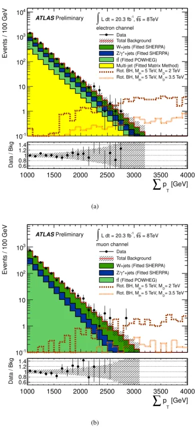
T <1500 GeV constitute a preselection sample from which special control regions and signal regions are defined by adding other selection criteria. Figure 1 shows the
Pp
Tdistribution for preselected events, for the electron and muon channels. The signal, containing multiple high-p
Tleptons and jets, would manifest itself as an excess of events at higher
Pp
T, and is entirely negligible in the preselection region.
700 800 900 1000 1100 1200 1300 1400 1500
Events / 20 GeV
1 10 102
103
104
Data Total Background W+jets (SHERPA) Multi-jets (Matrix Method)
*+jets (SHERPA) γ Z/
(POWHEG) t t
Single top (ACERMC/MCatNLO) Diboson (HERWIG)
[GeV]
T
∑
p700 800 900 1000 1100 1200 1300 1400 1500 Data / Bkg 0.60.811.21.4
ATLASPreliminary = 8 TeV s
-1, L dt = 20.3 fb
∫
electron channel
(a)
700 800 900 1000 1100 1200 1300 1400 1500
Events / 20 GeV
1 10 102
103
104
Data Total Background W+jets (SHERPA)
*+jets (SHERPA) γ Z/
(POWHEG) t t
Single top (ACERMC/MCatNLO) Diboson (HERWIG)
[GeV]
T
∑
p700 800 900 1000 1100 1200 1300 1400 1500 Data / Bkg 0.60.811.21.4
ATLASPreliminary = 8 TeV s
-1, L dt = 20.3 fb
∫
muon channel
(b)
Figure 1: The
Pp
T, after event preselection, in the electron (left) and muon (right) channels. The Monte
Carlo distributions are rescaled using scale factors derived in the appropriate control regions, as described
in the text. The lower panels show the ratio of the data to the expected background, with the statistical
uncertainty on data (points), and separately, the fractional total uncertainty on the background (shaded
band).
For the signal region, in order to reduce the SM background contributions, events are required to contain at least three reconstructed objects with p
T >100 GeV, at least one of which must be a lepton, as well as to have a minimum
Pp
Tof 2000 GeV. In each of the channels, the signal region above
Pp
T =2000 GeV is divided into multiple slices, with minimum
Pp
Tthresholds increasing in steps of 200 GeV. This allows the analysis to be sensitive across a wider range of signal models, and values of M
Dand M
th. Events at lower
Pp
T, but with otherwise the same requirements as the signal region, constitute a “sideband” region. The contributions from signal models not yet excluded by earlier analyses to the sideband region are well below 1%. The selection criteria for the sideband and signal regions are summarised in Table 2.
7 Background Estimation
The dominant sources of Standard Model background in this search are the production W and Z bosons in association with jets, t¯ t production and multi-jet processes. The leptonic decays of W, Z and top quarks produce events with real leptons, with associated high- p
Tjets (hereinafter called “prompt” backgrounds).
In multi-jet events, reconstructed leptons arise either from semi-leptonic decays within jets (dominantly from heavy flavour decays), or from mis-identification of a hadronic jet; collectively, these are denoted as “fake" leptons.
The backgrounds are estimated using a combination of data-driven and MC-based techniques. The multi-jet contribution is estimated using a data-driven technique that is more reliable than simulation for determining fake lepton backgrounds, due to its independence from MC modelling uncertainties such as hadronisation and detector simulation. Prompt backgrounds are estimated using MC samples, normalised in data control regions that are dominated by a single background component and kinematically close to the signal region.
At very high
Pp
T, the number of events in the simulated samples becomes more limited, and there- fore subject to statistical fluctuations. Therefore, for each background component, the
Pp
Tdistribution is fitted to a functional form to smooth the backgrounds and extrapolate them to very high
Pp
T. 7.1 Prompt background estimation from control regions
The background estimates for processes involving prompt leptons are based on MC simulations nor- malised in control regions, each dominated by a single process, as discussed above. The normalisation factors are determined, separately for the electron and muon channels, for the three main backgrounds:
Z
+jets, W
+jets and t¯ t. The control regions are defined in Table 3.
For the Z
+jets control region, events passing preselection requirements are then required to containtwo electrons or muons of opposite charge and to have di-lepton invariant mass between 80 and 100 GeV.
The W
+jets control region consists of events with exactly one lepton, no b-tagged jets and E
missTgreater than 60 GeV, where the last two requirements help to reduce the t¯ t and Z
+jets
/multi-jet contributions, respectively. The t¯ t control region consists of events with exactly one lepton and at least four jets, of
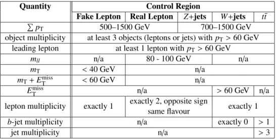
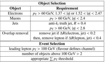
Quantity Region
Sideband Signal P
p
T1000–2000 GeV
>2000 GeV object multiplicity at least 3 objects above 100 GeV
leading lepton at least 1 lepton with p
T>100 GeV
Table 2: Definitions of the sideband and signal regions.
Quantity Control Region
Fake Lepton Real Lepton
Z
+jetsW
+jetst¯ t
P
p
T500–1500 GeV 700–1500 GeV
object multiplicity at least 3 objects (leptons or jets) with p
T >60 GeV leading lepton at least 1 lepton with p
T >60 GeV
m
lln
/a 80 - 100 GeV n
/a
m
T <40 GeV n
/a
m
T+E
missT <60 GeV n
/a
E
missTn
/a
>60 GeV n
/a
lepton multiplicity exactly 1 exactly 2, opposite sign
exactly 1 same flavour
b-jet multiplicity n
/a exactly 0
>1
jet multiplicity n
/a
>3
Table 3: Definitions of the SM background-dominated control regions as well as the real and fake en- hanced regions used in the data-driven multi-jet estimate.
which at least two must be tagged as b-jets. The final criterion ensures orthogonality to the W
+jet control region and preferentially selects for the top quark decays. The purities of the Z
+jets,W
+jetsand t¯ t control regions are estimated from Monte Carlo simulations to be about 98%, 70% and 90%, respectively.
The number of events predicted by the MC simulation is compared to the observed number of events in data in each of the control regions, to derive the scale factors used to normalise the backgrounds. Due to non-negligible contamination of W
+jets events in the t¯ t control region and vice-versa, two coupled equations determine the two normalisations that lead to agreement between data and MC simulation.
The derived scale factors to be applied to the background predictions in the electron (muon) channels are 1.00 (1.08) for t¯ t, 0.76 (0.81) for W
+jets, and 0.90 (0.93) for Z
+jets.
The much smaller contributions of single top and di-boson processes are estimated to comprise ap- proximately 2% and 0.5%, respectively, of the events in the sideband and signal regions. Their estimates are taken directly from Monte Carlo simulations.
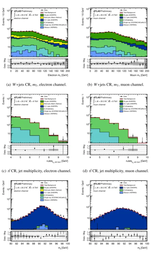
Figure 2 shows the good agreement obtained in kinematic distributions in the control regions. The
Pp
Tdistribution for each control region is shown in Figure 3, which demonstrates good modelling of the background shape.
7.2 Fake lepton background estimation
The multi-jet background is estimated with a data-driven matrix method, described in detail in Ref. [74].
The contribution from two or more fake leptons is found to be negligible. In order to make an estimate using this method, a multi-jet enhanced sample is obtained by relaxing the lepton selection criteria so as to increase the contribution from fake leptons. This is achieved in the electron channel by loosening the leading electron identification criteria from “tight" to “medium", and for the muon channel, by removing both the jet-muon overlap and muon isolation requirements.
The numbers of data events in the sample which pass (N
pass) and fail (N
fail) the nominal, tighter lepton selection criteria are counted. Defining N
promptand N
fakeas the numbers of events for which the leptons are prompt and fake, respectively, the following relationships hold:
N
pass=promptN
prompt+fakeN
fake,(3)
0 20 40 60 80 100 120 140 160 180 200
Events / 10 GeV
1 10 102
103
104
105 Data
Total Background W+jets (SHERPA) Multi-jets (Matrix Method)
*+jets (SHERPA) γ Z/
(POWHEG) t t
Single top (ACERMC/MCatNLO) Diboson (HERWIG)
[GeV]
Electron mT
0 20 40 60 80 100 120 140 160 180 200 Data / Bkg 0.60.811.21.4
ATLASPreliminary = 8 TeV s -1, L dt = 20.3 fb
∫
electron channel
(a)W+jets CR,mT, electron channel.
0 20 40 60 80 100 120 140 160 180 200
Events / 10 GeV
1 10 102
103
104
105 Data
Total Background W+jets (SHERPA)
*+jets (SHERPA) γ Z/
(POWHEG) t t
Single top (ACERMC/MCatNLO) Diboson (HERWIG)
[GeV]
Muon mT
0 20 40 60 80 100 120 140 160 180 200 Data / Bkg 0.60.811.21.4
ATLASPreliminary = 8 TeV s -1, L dt = 20.3 fb
∫
muon channel
(b)W+jets CR,mT, muon channel.
4 5 6 7 8 9 10
Events / 1
1 10 102
103
104
105
Data Total Background W+jets (SHERPA) Multi-jets (Matrix Method)
*+jets (SHERPA) γ Z/
(POWHEG) t t
Single top (ACERMC/MCatNLO) Diboson (HERWIG)
[GeV]
>60 GeV pT
nJets
4 5 6 7 8 9 10
Data / Bkg 0.60.811.21.4
ATLASPreliminary = 8 TeV s -1, L dt = 20.3 fb
∫
electron channel
(c) tt¯CR, jet multiplicity, electron channel.
4 5 6 7 8 9 10
Events / 1
1 10 102
103
104
105 DataTotal Background
W+jets (SHERPA)
*+jets (SHERPA) γ Z/
(POWHEG) t t
Single top (ACERMC/MCatNLO) Diboson (HERWIG)
[GeV]
>60 GeV pT
nJets
4 5 6 7 8 9 10
Data / Bkg 0.60.811.21.4
ATLASPreliminary = 8 TeV s -1, L dt = 20.3 fb
∫
muon channel
(d)tt¯CR, jet multiplicity, muon channel.
80 82 84 86 88 90 92 94 96 98 100
Events / GeV
1 10 102
103
104
Data Total Background W+jets (SHERPA) Multi-jets (Matrix Method)
*+jets (SHERPA) γ Z/
(POWHEG) t t
Single top (ACERMC/MCatNLO) Diboson (HERWIG)
[GeV]
mll
80 82 84 86 88 90 92 94 96 98 100 Data / Bkg 0.60.811.21.4
ATLASPreliminary = 8 TeV s -1, L dt = 20.3 fb
∫
electron channel
(e)Z+jets CR, di-lepton invariant mass, electron channel.
80 82 84 86 88 90 92 94 96 98 100
Events / GeV
1 10 102
103
104
Data Total Background
*+jets (SHERPA) γ Z/
(POWHEG) t t Diboson (HERWIG)
[GeV]
mll
80 82 84 86 88 90 92 94 96 98 100 Data / Bkg 0.60.811.21.4
ATLASPreliminary = 8 TeV s -1, L dt = 20.3 fb
∫
muon channel
(f) Z+jets CR, di-lepton invariant mass, muon channel.
Figure 2: Kinematic distributions for the three control regions. The Monte Carlo samples are normalised
to data using scale factors, according to the method described in Section 7. The regions are defined in
Table 3. The lower panels show the ratio of the data to the expected background, with the statistical
uncertainty on data (points), and separately, the fractional total uncertainty on the background (shaded
band).
700 800 900 1000 1100 1200 1300 1400 1500
Events / 20 GeV
10 102
103
Data Total Background W+jets (SHERPA) Multi-jets (Matrix Method)
*+jets (SHERPA) γ Z/
(POWHEG) t t
Single top (ACERMC/MCatNLO) Diboson (HERWIG)
[GeV]
T
∑ p 700 800 900 1000 1100 1200 1300 1400 1500 Data / Bkg 0.60.811.21.4
ATLASPreliminary = 8 TeV s -1, L dt = 20.3 fb
∫
electron channel
(a) Z+jets CR,P
pT, electron channel.
700 800 900 1000 1100 1200 1300 1400 1500
Events / 20 GeV
1 10 102
103
104 Data
Total Background W+jets (SHERPA) Multi-jets (Matrix Method)
*+jets (SHERPA) γ Z/
(POWHEG) t t
Single top (ACERMC/MCatNLO) Diboson (HERWIG)
[GeV]
T
∑ p 700 800 900 1000 1100 1200 1300 1400 1500 Data / Bkg 0.60.811.21.4
ATLASPreliminary = 8 TeV s -1, L dt = 20.3 fb
∫
electron channel
(b)W+jets CR,P
pT, electron channel.
700 800 900 1000 1100 1200 1300 1400 1500
Events / 20 GeV
10 102
103
Data Total Background W+jets (SHERPA)
*+jets (SHERPA) γ Z/
(POWHEG) t t
Single top (ACERMC/MCatNLO) Diboson (HERWIG)
[GeV]
T
∑ p 700 800 900 1000 1100 1200 1300 1400 1500 Data / Bkg 0.60.811.21.4
ATLASPreliminary = 8 TeV s -1, L dt = 20.3 fb
∫
muon channel
(c)t¯tCR,P
pT, muon channel.
Figure 3:
Pp
Tdistributions for each control region. The Monte Carlo samples are normalised to data using scale factors, according to the method described in Section 7. The regions are defined in Table 3.
The lower panels show the ratio of the data to the expected background, with the statistical uncertainty
on data (points), and separately, the fractional total uncertainty on the background (shaded band).
and
N
fail=(1
−prompt)N
prompt+(1
−fake)N
fake,(4) where
promptand
fakeare the relative efficiencies for prompt and fake leptons to pass the nominal se- lection, given they have passed the looser selection criteria. The simultaneous solution of these two equations gives a prediction for the number of events in data with fake leptons passing the nominal criteria, taken to be the estimated number of multi-jet events:
N
fake =N
fail−(1/
prompt−1)N
pass1
−fake/prompt .(5)
The efficiencies
promptand
fakeare determined from control regions enhanced in prompt lepton or fake lepton events, respectively, as described in Table 3. A fake-enhanced control sample is obtained by selecting events with exactly one lepton that satisfies the relaxed lepton criteria described above, m
T <40 GeV and m
T+E
missT <60 GeV. After observing no
Pp
Tdependence in
fakeand
prompt, the minimum
Pp
Trequirement for these regions is set to 500 GeV, compared with
Pp
T>700 GeV for the other control regions, in order to gain statistical power.
The efficiency for identifying fakes as prompt leptons is given by the fraction of the events in this control region that also pass the nominal lepton selection, after subtracting, in both instances, the es- timated contribution from prompt lepton backgrounds (derived from MC simulations, renormalised to match data in control regions, as described above). For the muon channel,
fakeis found to be negligibly small, consistent with zero: 0.0043± 0.0040 (stat), or
<0.011 at 95% CL. For the electron channel, some dependence on the p
Tand
ηof the leading electron is observed, which is taken into account by using p
T-
and
η-dependentfake; they vary in the range 0.26–0.42.
The e
fficiency
promptis evaluated in a region with the same selection as the Z
+jets control region, except for the relaxed
Pp
Trequirement, 500 GeV
< Pp
T <1500 GeV, to match that used in the fake lepton control region. The relative efficiency for identifying prompt leptons is obtained through the ratio of the number of events in which both leptons pass the nominal selection to those in which only one does.
The measured values of
promptare 0.960± 0.007 and 0.942± 0.007 for electrons and muons, respectively, where the quoted uncertainties are statistical only.
7.3 Background smoothing with fits At high
Pp
T, particularly beyond
Pp
T ≈3500 GeV, the numbers of events in the simulated background samples are small and consequently have large statistical uncertainties. To provide a more robust predic- tion in the signal region, the
Pp
Tdistributions of each individual background are fitted to an empirical function that enables the background shape to be smoothed and extended without being strongly affected by statistical fluctuations. This method reduces the statistical uncertainty, by using information at lower
Pp
Tto constrain the shape of the distribution, but introduces systematic uncertainties from the choice of binning and normalisation region, and from choice of fit function. These are further discussed in Section 8. The fit function used is given by:
F =
(1
−x)
p0x
p1x
p2log(x),(6)
where x
= Pp
T/√s, and p
0,p
1and p
2are the parameters to be fitted. The function was chosen for its stable and reliable description of the shape of the distributions over the full range of
Pp
T. In previous studies [75–77], ATLAS and other experiments have found that this ansatz provides satisfactory fits to kinematic distributions. The fit range begins at
Pp
T =700 GeV, and ends where the number of simulated
events in a given bin is below five. The start- and end-points of the fit range, as well as the binning, are
varied, and the results are consistent with the nominal fit within the statistical uncertainty. Although the
default fits (shown in Figures 4 and 5) are of high quality and stability, there is an uncertainty associated
with the choice of background fit function. To assess this, an alternate function was chosen that succeeds in describing the distributions at low and intermediate
Pp
Tbut has a di
fferent shape than the nominal function at high
Pp
T, where the numbers of simulated events are smaller. This function is given by:
Falt=
p
0x (1
−p
1x)
p2 ,(7)
where x
=Pp
T/√s, and p
0,p
1and p
2are the parameters to be fitted.
In the bins where the prediction from this alternate function falls outside the nominal fit uncertainty, the di
fference between the nominal and alternate functions is used as the fit uncertainty, i.e. an enve- lope of them is taken and symmetrised, to be conservative, ensuring that the total fit uncertainty covers alternate functions and the inherent uncertainty of the fit itself.
The
Pp
Tdistributions for each MC-simulated prompt lepton background are displayed in Figure 4;
the curves shown represent the results of the binned maximum likelihood fits. The multi-jet background in the electron channel estimated from data is fitted to the same function, as shown in Figure 5. The fit quality is high, with typical
χ2/d.o.f. values between 0.9 and 1.6.
The fitted shapes of the individual backgrounds are combined according to their relative predicted contributions (as discussed in the preceding sections, computed in a subset of the sideband region, 1000
<P
p
T <1500 GeV) to give an overall background template shape. In order to reduce the systematic uncertainty, this is normalised to data in this region by a minimisation of the
χ2di
fference between the data and the background template. This results in a normalisation consistent with that determined from the control regions within the 4% uncertainty resulting from the statistical uncertainty on the data in these bins. The resulting background estimate gives a smooth and stable prediction at all values of
Pp
T.
Events / 100 GeV
10-2 10-1 1 10 102
103 Z/γ*+jets (SHERPA)
Fit + Total uncertainty
[GeV]
T
∑ p 1000 1500 2000 2500 3000 3500 4000
MC / Fit
0.60.81 1.2 1.4
ATLASPreliminary Simulation electron channel
s T/ p Σ , x = log(x) p2
x p1 0 x p (1-x) Fit Parameters:
0.9
± : 14.3 p0
0.28 : -4.43 ± p1
0.1
± : -0.35 p2
(a)
Events / 100 GeV
10-2 10-1 1 10 102 103
*+jets (SHERPA) γ Z/
Fit + Total uncertainty
[GeV]
T
∑ p 1000 1500 2000 2500 3000 3500 4000
MC / Fit
0.60.81 1.2 1.4
ATLASPreliminary Simulation muon channel
s T/ p Σ , x = log(x) p2
x p1 0 x p (1-x) Fit Parameters:
0.4
± : 16.1 p0
0.12 : -4.42 ± p1
0.04
± : -0.39 p2
(b)
Events / 100 GeV
10-2 10-1 1 10 102
103 W+jets (SHERPA)
Fit + Total uncertainty
[GeV]
T
∑ p 1000 1500 2000 2500 3000 3500 4000
MC / Fit
0.6 0.81 1.21.4
ATLASPreliminary Simulation electron channel
s T/ p Σ , x = log(x) p2
x p1 0 x p (1-x) Fit Parameters:
0.3
± : 13.3 p0
0.08
± : -4.98 p1
0.03
± : -0.43 p2
(c)
Events / 100 GeV
10-2 10-1 1 10 102
103 W+jets (SHERPA)
Fit + Total uncertainty
[GeV]
T
∑ p 1000 1500 2000 2500 3000 3500 4000
MC / Fit
0.6 0.81 1.21.4
ATLASPreliminary Simulation muon channel
s T/ p Σ , x = log(x) p2
x p1 0 x p (1-x) Fit Parameters:
0.3
± : 12.6 p0
0.10
± : -4.54 p1
0.04
± : -0.33 p2
(d)
Events / 100 GeV
10-2 10-1 1 10 102
103 tt (POWHEG)
Fit + Total uncertainty
[GeV]
T
∑ p 1000 1500 2000 2500 3000 3500 4000
MC / Fit
0.6 0.81 1.2 1.4
ATLASPreliminary Simulation electron channel
s T/ p Σ , x = log(x) p2
x p1
x
0 p (1-x) Fit Parameters:
0.3
± : 17.5 p0
0.08
± : -5.48 p1
0.03
± : -0.67 p2
(e)
Events / 100 GeV
10-2 10-1 1 10 102 103
(POWHEG) t t
Fit + Total uncertainty
[GeV]
T
∑ p 1000 1500 2000 2500 3000 3500 4000
MC / Fit
0.6 0.81 1.2 1.4
ATLASPreliminary Simulation muon channel
s T/ p Σ , x = log(x) p2
x p1
x
0 p (1-x) Fit Parameters:
0.4
± : 19.5 p0
0.10
± : -5.34 p1
0.04
± : -0.65 p2
(f)
Figure 4: The
Pp
Tdistributions and fit curves for Z
+jets (a), (b);W
+jets (+di-boson) (c), (d); and t¯ t (+
single top) (e), (f) MC-simulated events. Distributions for the electron channel are on the left while those for the muon channel are on the right. The shaded bands on the fit curves reflect the total uncertainty on the fit, including the systematic uncertainty discussed in Section 7.3. The length of the black line indicates the
Pp
Trange fitted. The lower panels show the ratio of the MC prediction to the fit, with the
statistical uncertainty on the MC prediction (points), and separately, the fractional uncertainty on the fit
(shaded band).
Events / 100 GeV
10-2
10-1
1 10 102
103 Multi-jet (Matrix Method)
Fit + Total uncertainty
[GeV]
T
∑
p1000 1500 2000 2500 3000 3500 4000
Prediction / Fit
0.6 0.81 1.2 1.4
ATLASPreliminary electron channel
s
T/ p , x = Σ
log(x) p2
x
p1 0 x
p
(1-x) Fit Parameters:
2.0 : 15.2 ± p0
0.60 : -4.82 ± p1
0.22 : -0.45 ± p2