Search for squarks and gluinos with the ATLAS detector in final states with jets and missing transverse momentum and 20.3 fb

ATLAS-CONF-2013-047 30/06/2013

ATLAS NOTE

ATLAS-CONF-2013-047

May 16, 2013 Revision: June 30, 2013

Search for squarks and gluinos with the ATLAS detector in final states with jets and missing transverse momentum and 20.3 fb

⁻¹

of √

s = 8 TeV proton-proton collision data

ATLAS Collaboration

Abstract

A search for squarks and gluinos in final states containing high-p

_T

jets, missing trans- verse momentum and no electrons or muons is presented. The data were recorded in 2012 by the ATLAS experiment in

√

s =

8 TeV proton-proton collisions at the Large Hadron Collider, with a total integrated luminosity of 20.3 fb

⁻¹

. No significant excess above the Standard Model expectation is observed. In a simplified model with only gluinos and the lightest neutralino, gluino masses below 1350 GeV are excluded at the 95% confidence level when the lightest neutralino is massless. For a simplified model involving the strong pro- duction of squarks of the first two generations, with decays to a massless lightest neutralino, squark masses below 780 GeV are excluded. In MSUGRA/CMSSM models with tan

β=

30,

A₀ = −2m₀

and

µ >

0, squarks and gluinos of equal mass are excluded for masses below 1700 GeV. These limits extend the region of supersymmetric parameter space excluded by previous searches with the ATLAS detector.

The following have been revised with respect to the version dated May 16, 2013:

squark mass contours in Figures 5 and 16 (left), m_g˜−mq_˜ plane exclusion limits in Figures 5 and 16 (right) and mass limit values for the MSUGRA/CMSSM scenario; cross-sections and resulting exclusion limits for the simplified phenomenological MSSM scenario (Figures

6 and 17).

c

Copyright 2013 CERN for the benefit of the ATLAS Collaboration.

1 Introduction

Many extensions of the Standard Model (SM) include heavy coloured particles, some of which could be accessible at the Large Hadron Collider (LHC) [1]. The squarks and gluinos of supersymmetric (SUSY) theories [2–10] form one class of such particles. This note presents a new ATLAS search for squarks and gluinos in final states containing only jets and large missing transverse momentum. Interest in this final state is motivated by the large number of R-parity conserving models [11–15] in which squarks, ˜ q, and gluinos, ˜

g, can be produced in pairs {g

˜

g, ˜

˜ q q, ˜ ˜ q

g}

˜ and can decay through ˜ q

→

q

χ

˜

⁰₁

and ˜

g →

q q ¯

χ

˜

⁰₁

to weakly interacting lightest neutralinos, ˜

χ⁰₁

. The ˜

χ⁰₁

is the lightest SUSY particle (LSP) and escapes the detector unseen. The analysis presented here updates previous ATLAS results obtained using similar selections [16–19]. Events with reconstructed electrons or muons are vetoed to avoid overlap with a related ATLAS search [20, 21]. The search strategy was optimised in the (m

g_˜,

m

_q˜

)-plane (where m

_g˜,

m

_q˜

are the gluino and squark masses respectively) for a range of models, including a simplified one in which all other supersymmetric particles, except for the lightest neutralino, were given masses beyond the reach of the LHC. Although mostly interpreted in terms of SUSY models, the main results of this analysis (the data and expected background event counts in the signal regions) are relevant for constraining any model of new physics that predicts production of jets in association with missing transverse momentum.

2 The ATLAS Detector and Data Samples

The ATLAS detector [22] is a multipurpose particle physics detector with a forward-backward sym- metric cylindrical geometry and nearly 4π coverage in solid angle.

¹

The layout of the detector fea- tures four superconducting magnet systems, which comprise a thin solenoid surrounding inner track- ing detectors (covering

|η| <

2.5) and three large toroids supporting a muon spectrometer (covering

|η| <

2.5). The calorimeters are of particular importance to this analysis. In the pseudorapidity region

|η|<

3.2, high-granularity liquid-argon (LAr) electromagnetic (EM) sampling calorimeters are used. An iron/scintillator-tile calorimeter provides hadronic coverage over

|η| <

1.7. The end-cap and forward regions, spanning 1.5

< |η| <

4.9, are instrumented with LAr calorimeters for both EM and hadronic measurements.

The data sample used in this analysis was collected in 2012 with the LHC operating at a centre- of-mass energy of 8 TeV. Application of beam, detector and data-quality requirements resulted in a total integrated luminosity of 20.3 fb

⁻¹

. The uncertainty on the integrated luminosity is

±2.8%, derived

by following the same methodology as that detailed in Ref. [23] using a preliminary calibration of the luminosity scale derived from beam-separation scans performed in November 2012. The trigger required events to contain a leading jet with an uncorrected transverse momentum ( p

_T

) above 80 GeV and an uncorrected missing transverse momentum above 100 GeV. The trigger reached its full efficiency for events with a reconstructed jet with p

_T

exceeding 130 GeV and more than 160 GeV of missing transverse momentum. For the data sample studied the trigger is fully e

ffi

cient.

3 Object Reconstruction

Jet candidates are reconstructed using the anti-k

t

jet clustering algorithm [24, 25] with a radius parameter of 0.4. The inputs to this algorithm are clusters [26, 27] of calorimeter cells seeded by those with energy significantly above the measured noise. Jet momenta are constructed by performing a four-vector sum

1ATLAS uses a right-handed coordinate system with its origin at the nominal interaction point in the centre of the detector

and thez-axis along the beam pipe. Cylindrical coordinates (r, φ) are used in the transverse plane,φbeing the azimuthal angle

around the beam pipe. The pseudorapidityηis defined in terms of the polar angleθbyη=−ln tan(θ/2).

over these cell clusters, treating each as an (E, ~ p) four-vector with zero mass. The jets are corrected for energy from additional proton-proton collisions in the same or neighbouring bunch crossings (pile-up) using a method, suggested in Ref. [28], which estimates the pile-up activity in any given event, as well as the sensitivity of any given jet to pile-up. The method subtracts a contribution from the jet energy equal to the product of the jet area and the event average energy density. The local cluster weighting (LCW) jet calibration method [26, 29] is used to classify topological cell clusters within the jets as either being of electromagnetic or hadronic origin and based on this classification applies specific energy corrections derived from a combination of Monte Carlo (MC) simulation and data. Further corrections, referred to as ‘jet energy scale’ or ‘JES’ corrections below, are derived from MC and data and used to calibrate the energies of jets to the mean scale of their constituent particles [26]. Only jet candidates with p

_T >

20 GeV after all corrections are retained. Jets are identified as originating from heavy-flavour decays using the

‘MV1’ neural network based b-tagging algorithm with a 70% efficiency operating point [30]. Candidate b-tagged jets must possess p

_T >

40 GeV and

|η|<

2.5.

Electron candidates are required to have p

_T >

10 GeV and

|η| <

2.47, and to pass electron shower shape and track selection criteria based upon those described in Ref. [31], but modified to reduce the impact of pile-up and to match tightened trigger requirements. Muon candidates are formed by combin- ing information from the muon spectrometer and inner tracking detectors as described in Refs. [32, 33]

and are required to have p

_T >

10 GeV and

|η| <

2.4. Reconstructed photons are used to constrain Z

+

jet backgrounds (see below), although they are not used in the main analysis. Photon candidates are required to possess p

_T >

130 GeV and

|η| <

1.37 or 1.52

< |η| <

2.47, and to pass photon shower shape and electron rejection criteria [34].

Following the steps above, overlaps between candidate jets with

|η| <

2.8 and leptons (electrons or muons) are resolved as follows. First, any such jet candidate lying within a distance

∆

R

≡ p

(

∆η)²+

(

∆φ)² =

0.2 of an electron is discarded; then any lepton candidate remaining within a distance

∆

R

=

0.4 of any surviving jet candidate is discarded.

The measurement of the missing transverse momentum two-dimensional vector

E^miss_T

(and its magni- tude E

_T^miss

) is based on the calibrated transverse momenta of all jet and lepton candidates and all calorime- ter clusters not associated to such objects [35]. Following this step, all jet candidates with

|η| >

2.8 are discarded. Thereafter, the remaining lepton and jet candidates are considered “reconstructed”, and the term “candidate” is dropped.

4 Signal and Control Region Definitions

Following the object reconstruction described above, events are discarded if any electrons or muons with p

_T >

10 GeV remain, or if they have any jets failing quality selection criteria designed to suppress detector noise and non-collision backgrounds (see e.g. Ref. [36]), or if they lack a reconstructed primary vertex associated with five or more tracks. The criteria applied to jets include requirements on the fraction of the transverse momentum of the jet carried by charged tracks, and on the fraction of the jet energy contained in the electromagnetic layers of the calorimeter. A consequence of these requirements is that events containing hard photons have a high probability of failing the signal region selection criteria.

This analysis aims to search for the production of heavy SUSY particles decaying into jets and stable

lightest neutralinos, with the latter creating missing transverse momentum. Because of the high mass

scale expected for the SUSY signal, the ‘e

ff

ective mass’, m

_eff

, is a powerful discriminant between the

signal and most Standard Model backgrounds. When selecting events with at least N jets, m

_eff

is defined

to be the scalar sum of the transverse momenta of the leading N jets and E

^miss_T

. The final signal selection

uses requirements on m

_eff

(incl.), which sums over all jets with p

_T >

40 GeV and E

^miss_T

. Requirements

placed on m

_eff

and E

_T^miss

, which suppress the multi-jet background, formed the basis of the previous

ATLAS jets

+

E

^miss+

0-lepton SUSY searches [17–19]. The same strategy is adopted in this analysis.

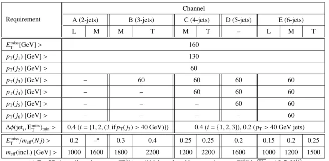
Requirement

Channel

A (2-jets) B (3-jets) C (4-jets) D (5-jets) E (6-jets)

L M M T M T – L M T

E^miss_T [GeV]> 160

pT(j1) [GeV]> 130

pT(j2) [GeV]> 60

pT(j3) [GeV]> – 60 60 60 60

pT(j4) [GeV]> – – 60 60 60

pT(j5) [GeV]> – – – 60 60

pT(j6) [GeV]> – – – – 60

∆φ(jet_i,E^miss_T )min> 0.4 (i={1,2,(3 ifpT(j3)>40 GeV)}) 0.4 (i={1,2,3}), 0.2 (pT>40 GeV jets)

E^miss_T /m_eff(N j)> 0.2 –^a 0.3 0.4 0.25 0.25 0.2 0.15 0.2 0.25

meff(incl.) [GeV]> 1000 1600 1800 2200 1200 2200 1600 1000 1200 1500

(a) For SR A-medium the cut onE_T^miss/m_eff(N j) is replaced by a requirementE^miss_T /√

HT>15 GeV^1/2.

Table 1: Selection criteria used to define each of the channels in the analysis. Each channel is divided into between one and three signal regions on the basis of the requirements listed in the bottom two rows.

The signal regions are indicated in the third row from the top and are denoted ‘loose’ (L), ‘medium’

(M) and ‘tight’ (T). The E

^miss_T /m_eff

cut in any N jet channel uses a value of m

_eff

constructed from only the leading N jets (indicated in parentheses in the second row). However, the final m

_eff

(incl.) selection, which is used to define the signal regions, includes all jets with p

_T >

40 GeV.

The requirements used to select jets and leptons are chosen to give sensitivity to a broad range of SUSY models. In order to achieve maximal reach over the (m

_g˜,

m

q_˜

)-plane, several analysis channels are defined. Squarks typically generate at least one jet in their decays, for instance through ˜ q

→

q

χ

˜

⁰₁

, while gluinos typically generate at least two jets, for instance through ˜

g →

q q ¯

χ

˜

⁰₁

. Processes contributing to

˜

q q, ˜ ˜ q

g

˜ and ˜

g˜g

final states therefore lead to events containing at least two, three or four jets, respectively.

Decays of heavy SUSY and SM particles produced in ˜ q and ˜

g

cascades tend to further increase the final state multiplicity.

Five inclusive analysis channels, labelled A to E and characterised by increasing jet multiplicity from two to six, are defined in Table 1. Each channel is used to construct between one and three signal regions (SRs) with ‘loose’, ‘medium’, or ‘tight’ selections distinguished by requirements placed on E

^miss_T /m_eff

and m

_eff

(incl.). The lower jet multiplicity channels focus on models characterised by squark pair pro- duction with short decay chains, while those requiring high jet multiplicity are optimised for gluino pair production and/or long cascade decay chains. In SR A-medium the cut on E

_T^miss/m_eff

is replaced by a requirement on E

_T^miss/√

H

_T

(where H

_T

is defined as the scalar sum of the transverse momenta of all p

_T >

40 GeV jets), which has been found to lead to enhanced sensitivity to models characterised by ˜ q q ˜ production with a large ˜ q– ˜

χ⁰₁

mass splitting.

In Table 1,

∆φ(jet,E^miss_T

)

min

is the smallest of the azimuthal separations between

E^miss_T

and the re- constructed jets. For channels A and B, the selection requires

∆φ(jet,E^miss_T

)

min >

0.4 using up to three leading jets with p

_T >

40 GeV if present in the event. For the other channels an additional requirement

∆φ(jet,E^miss_T

)

_min >

0.2 is placed on all jets with p

_T >

40 GeV. Requirements on

∆φ(jet,E^miss_T

)

_min

and E

^miss_T /m_eff

are designed to reduce the background from multi-jet processes.

Standard Model background processes contribute to the event counts in the signal regions. The

dominant sources are: W

+

jets, Z

+

jets, top quark pairs, single top quarks, and multiple jets. The produc-

tion of semi-leptonically decaying dibosons is a small component (<13%) of the total background and

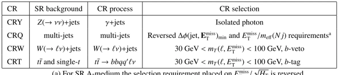
CR SR background CR process CR selection

CRY Z(→νν)+jets γ+jets Isolated photon

CRQ multi-jets multi-jets Reversed∆φ(jet,E^miss_T )minandE^miss_T /m_eff(N j) requirements^a

CRW W(→`ν)+jets W(→`ν)+jets 30 GeV<mT(`,E^miss_T )<100 GeV,b-veto

CRT tt¯and single-t tt¯→bbqq⁰`ν 30 GeV<mT(`,E_T^miss)<100 GeV,b-tag

(a) For SR A-medium the selection requirement placed onE_T^miss/√

HTis reversed.

Table 2: Control regions used in the analysis: the main targeted background in the SR, the process used to model the background, and main CR cut(s) used to select this process are given. The transverse momenta of leptons(photons) used to select CR events must exceed 25(130) GeV.

is estimated with MC simulated data normalised to theoretical cross-section predictions. The majority of the W

+

jets background is composed of W

→ τν

events, with the

τ-lepton decaying to hadrons, or

W

→

eν, µν events in which no electron or muon candidate is reconstructed. The largest part of the Z

+

jets background comes from the irreducible component in which Z

→ν¯ν

decays generate large E

_T^miss

. Top quark pair production followed by semi-leptonic decays, in particular t¯ t

→

b bτνqq ¯

⁰

with the

τ-lepton

decaying to hadrons, as well as single top quark events, can also generate large E

^miss_T

and pass the jet and lepton requirements at a non-negligible rate. The multi-jet background in the signal regions is caused by misreconstruction of jet energies in the calorimeters leading to apparent missing transverse momentum, as well as by neutrino production in semileptonic decays of heavy quarks. Extensive validation of the Monte Carlo simulation against data has been performed for each of these background sources and for a wide variety of control regions (CRs).

To estimate the backgrounds in a consistent and robust fashion, four control regions are defined for each of the 10 signal regions, giving 40 CRs in total. The orthogonal CR event selections are designed to provide independent data samples enriched in particular background sources. Each ensemble of one SR and four CRs constitutes a different ‘stream’ of the analysis. The CR selections are optimised to maintain adequate statistical weight and low SUSY signal contamination, while minimising as far as possible the systematic uncertainties arising from the extrapolation to the SR.

The CRs are listed in Table 2. CRY is used to estimate the contribution of Z(

→νν)+jets background

events to each SR by selecting a sample of

γ+jets events with

p

_T

(γ)

>

130 GeV. CRQ uses reversed selection requirements placed on

∆φ(jet,E^miss_T

)

_min

and on E

_T^miss/m_eff

(N j) (E

^miss_T /√

H

_T

in SR A-medium) to produce data samples enriched in multi-jet background events. CRW and CRT use respectively a b-jet veto or b-jet requirement together with a requirement on the transverse mass (m

T

) of a p

_T >

25 GeV lepton and E

_T^miss

to select samples of W(→

`ν)+

jets and semi-leptonic t¯ t background events. These sam- ples are used to estimate respectively the W

+jets and combined

t¯ t and single-top background populations.

With the exception of SR A-loose, the CRW and CRT selections do not use the SR selection requirements applied to

∆φ(jet,E^miss_T

)

_min

or E

_T^miss/m_eff

(N j) (E

_T^miss/√

H

_T

in SR A-medium) in order to increase CR data

event statistics without significantly increasing theoretical uncertainties associated with the background

estimation procedure. For the same reason the final m

_eff

(incl.) requirements are loosened to 1300 GeV

in CRW and CRT for signal regions D and E-tight. Cross-checks are performed using several ‘validation

region’ samples selected with requirements minimally correlated with those used in the CRs. For exam-

ple, CRY estimates of the Z(→

ν¯ν)+jets background are validated with samples of

Z(→

``)+jets events

selected by requiring lepton pairs of opposite sign and identical flavour for which the di-lepton invariant

mass lies within 25 GeV of the mass of the Z boson. The results of these cross-checks are found to be

consistent with background expectations obtained from the CRs described above.

5 Analysis procedure

The observed numbers of events in the CRs for each SR are used to generate internally consistent SM background estimates for the SR via a likelihood fit. This procedure enables CR correlations due to common systematic uncertainties and contamination by other SM processes and/or SUSY signal events to be taken into account. The same fit also allows the statistical significance of the observation in the SR to be determined. Key ingredients in the fit are the ratios of expected event counts (the transfer factors TFs) from each background process between the SR and each CR, and between CRs. The TFs enable observations in the CRs to be converted into background estimates in the SR using:

N(SR, scaled)

=

N(CR, obs)

×

"

N(SR, unscaled)

N(CR, unscaled)

#

,

(1)

where N(SR, scaled) is the estimated background contribution to the SR by a given process, N(CR, obs) is the observed number of data events in the CR for the process, and N(SR, unscaled) and N(CR, unscaled) are a priori estimates of the contributions from the process to the SR and CR, respectively. The ratio appearing in the square brackets in Eqn. 1 is defined to be the transfer factor TF. Similar equations containing inter-CR TFs enable the background estimates to be normalised coherently across all the CRs in a given stream.

Background estimation requires determination of the central expected values of the TFs for each SM process, together with their associated correlated and uncorrelated uncertainties. The multi-jet TFs are estimated using a data-driven technique [17], which applies a resolution function to well-measured multi- jet events in order to estimate the impact of jet energy mismeasurement and heavy-flavour semileptonic decays on E

^miss_T

and other variables. The other TF estimates use fully simulated Monte Carlo samples validated with data. Some systematic uncertainties, for instance those arising from the jet energy scale (JES), or theoretical uncertainties in MC cross-sections, largely cancel when calculating the event count ratios constituting the TFs.

The result of the likelihood fit for each SR-CR ensemble is a set of background estimates and un- certainties for the SR together with a p-value giving the probability for the hypothesis that the SR event count is compatible with background alone. However, an assumption has to be made about the migration of signal events between regions. When searching for a signal in a particular SR, first it is assumed that the signal contributes only to the SR, i.e. the signal TFs are all set to zero, giving no contribution from the signal in the CRs. If no excess is observed, then limits are set within specific SUSY model planes, taking into account the contribution of signal in the CRs and the theoretical and experimental uncertainties on the SUSY production cross-section and kinematic distributions. Exclusion limits are obtained using a likelihood test which compares the observed event rates in the signal regions with the fitted background expectation and expected signal contribution for a given model.

Monte Carlo samples are used to develop the analysis, optimise the selections, determine the transfer factors used to estimate the W

+

jets, Z

+

jets and top quark backgrounds, determine the diboson back- grounds, and to assess the sensitivity to specific SUSY signal models. The following MC generators are used:

•

Samples of Z/γ

^∗

and

γ

events with accompanying jets are generated with SHERPA [37] with mas- sive b and c quarks. Theoretical uncertainties are evaluated by comparison with samples produced using ALPGEN [38].

•

Samples of W events with accompanying jets are generated with ALPGEN. Theoretical uncertainties are evaluated by comparison with samples produced using SHERPA.

•

Samples of top quark pair events with accompanying jets, assuming m

_top =

172.5 GeV, are gen-

erated with MC@NLO [39, 40]. Theoretical uncertainties are evaluated by comparison with samples

produced using SHERPA, POWHEG [41, 42] interfaced to PYTHIA6 [43], or POWHEG interfaced to HERWIG [44, 45] using JIMMY [46] for the underlying event.

•

Samples of single top quark events with accompanying jets are generated with MC@NLO [47, 48] for the s-channel and Wt processes and AcerMC [49] interfaced to PYTHIA6 for the t-channel process.

•

Samples of top quark pair events with accompanying jets and a W or Z boson are generated with MADGRAPH [50, 51] and PYTHIA6.

•

Samples of WZ, ZZ and Zγ events are generated with SHERPA, while samples of WW and Wγ events are generated with ALPGEN. The samples are normalised to the Next-to-Leading Order (NLO) cross-sections obtained from MCFM [52], except for the

ν¯νqq, `<sup>+</sup>`⁻

qq, Zγ and Wγ final states which are normalised to Leading Order (LO) cross-sections, with the resulting scale depen- dence (.25%) included in the theoretical uncertainties on these processes. Samples of WWW , WWZ and WWW events are generated with MADGRAPH and PYTHIA6, however their contribution is found to be null or negligible in all regions and hence they have not been used in the analysis.

Fragmentation and hadronisation for all ALPGEN and MC@NLO samples is performed with HERWIG, using JIMMY for the underlying event. The NLO PDF set CT10 [53] is used with SHERPA, MC@NLO and POWHEG, while the LO PDF set CTEQ6L1 [54] is used with all other generators.

SUSY signal samples are generated with HERWIG++ [55] or MadGraph

/

PYTHIA6 using PDF set CTEQ6L1. Signal cross-sections are calculated to next-to-leading order in the strong coupling constant, including the resummation of soft gluon emission at next-to-leading-logarithmic accuracy (NLO+NLL) [56–60].

The MC samples are generated using the same parameter set as Refs. [61–63]. Most SM background samples are passed through the ATLAS detector simulation [64] based on GEANT4 [65], while SHERPA W/Z

+jets and SUSY signal samples are passed through a fast simulation using a parameterisation of the

performance of the ATLAS electromagnetic and hadronic calorimeters. The fast simulation of SUSY signal events has been validated against full GEANT4 simulation for several signal model points. Differ- ing pile-up (multiple proton-proton interactions in a given event) conditions as a function of the LHC instantaneous luminosity are taken into account by overlaying simulated minimum-bias events generated with PYTHIA8 onto the hard-scattering process and reweighting them according to the mean number of interactions expected.

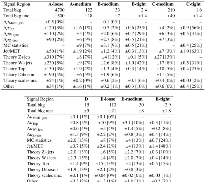
6 Systematic Uncertainties

Systematic uncertainties arise through the use of the transfer factors relating observations in the control regions to background expectations in the signal regions, and from the MC modelling of minor back- grounds and the SUSY signal.

Systematic uncertainties in the background estimates are presented in Table 3. For the MC-derived transfer factors the primary common sources of systematic uncertainty are the jet energy scale (JES) calibration, jet energy resolution (JER), theoretical uncertainties, MC statistics and the reconstruction performance in the presence of pile-up. In all cases correlations between uncertainties (for instance between scale uncertainties in CRs and SRs) are taken into account where appropriate.

The JES uncertainty has been measured using the techniques described in Refs. [26, 66], leading to

a slight dependence upon p

_T

and

η. The JER uncertainty is estimated using the methods discussed in

Ref. [67]. Contributions are added to both the JES and the JER uncertainties to account for the effect

of pile-up at the relatively high luminosity delivered by the LHC in the 2012 run. A further uncertainty

on the low- p

_T

calorimeter activity included in the E

^miss_T

calculation is taken into account. The combined

Signal Region

A-loose A-medium B-medium B-tight C-medium C-tight

Total bkg 4700 122 33 2.4 210 1.6

Total bkg unc.

±500 ±18 ±7 ±1.4 ±40 ±1.4

∆µ_Multi−jets ±

0.5 [0%] –

±

0.1 [0%] – – –

∆µ_Top ±120 [3%] ±1.6 [1%] ±0.7 [2%] ±0.6 [25%] ±4 [2%] ±0.9 [56%]

∆µ_W+jets ±110 [2%] ±5 [4%] ±2.0 [6%] ±0.7 [29%] ±6 [3%] ±0.5 [31%]

∆µ_Z+jets ±

90 [2%]

±

6 [5%]

±

2.7 [8%]

±

0.5 [21%]

±

7 [3%] –

MC statistics –

±9 [7%] ±3.1 [9%] ±0.5 [21%]

–

±0.4 [25%]

Jet

/

MET

±50 [1%] ±1.9 [2%] ±1.2 [4%] ±0.3 [13%] ±7 [3%] ±1.0 [63%]

Theory Z+jets

±

310 [7%]

±

8 [7%]

±

4 [12%]

±

0.1 [5%]

±

27 [13%] – Theory W+jets

±230 [5%] ±9 [7%] ±2.6 [8%] ±1.0 [42%] ±17 [8%] ±0.5 [31%]

Theory Top

±130 [3%] ±1.9 [2%] ±1.3 [4%] ±0.3 [14%] ±10 [5%] ±0.4 [25%]

Theory Diboson

±

190 [4%]

±

6 [5%]

±

1.9 [6%] –

±

11 [5%] –

Theory scales unc.

±24 [1%] ±0.2 [0%] ±0.6 [2%] ±0.1 [6%] ±0.4 [0%] ±0.03 [2%]

Other

±34 [1%] ±1.6 [1%] ±0.2 [1%] ±0.3 [10%] ±0.6 [0%] ±0.4 [25%]

Signal Region

D E-loose E-medium E-tight

Total bkg 15 113 30 2.9

Total bkg unc.

±5 ±21 ±8 ±1.8

∆µMulti−jets ±0.1 [1%] ±0.1 [0%]

– –

∆µ_Top ±0.8 [5%] ±10 [9%] ±3.1 [10%] ±0.3 [11%]

∆µ_W+jets ±0.6 [4%] ±5 [4%] ±1.4 [5%] ±0.2 [8%]

∆µZ+jets ±1.3 [9%] ±2.2 [2%] ±0.8 [3%] ±0.4 [14%]

MC statistics

±2.0 [13%] ±8 [7%] ±4 [13%] ±0.7 [24%]

Jet/MET

±0.7 [5%] ±2.4 [2%] ±4 [13%] ±1.4 [48%]

Theory Z+jets

±2.0 [13%] ±6 [5%] ±2.2 [7%] ±0.3 [10%]

Theory W

+

jets

±2.3 [15%] ±4 [4%] ±2.0 [7%] ±0.4 [14%]

Theory Top

±

1.4 [9%]

±

15 [13%]

±

4 [13%]

±

0.5 [17%]

Theory Diboson

±1.9 [13%] ±2.1 [2%] ±0.8 [3%]

–

Theory scales unc.

±0.1 [1%] ±0.04 [0%] ±0.02 [0%] ±0.03 [1%]

Other

±

0.3 [2%]

±

1.3 [1%]

±

1.0 [3%]

±

0.2 [7%]

Table 3: Breakdown of the dominant components of the systematic uncertainties on background esti-

mates. Hyphens indicate negligible contributions. Note that components may be correlated and hence

may not sum quadratically to the total background uncertainty.

∆µ

uncertainties arise from limited CR

statistics and systematic uncertainties related to the CR. Uncertainties relative to the expected total back-

ground yields are listed in parenthesis.

JES, JER and E

^miss_T

uncertainty ranges from 2% of the expected background in SR E-loose to 63% in SR C-tight (where it dominates).

Uncertainties arising from theoretical models of background processes are evaluated by comparing TFs obtained from samples generated with a variety of different MC generators, as described in Section 5.

In addition, the impact of uncertainties in renormalisation, factorisation and jet-parton matching scales is assessed with dedicated MC samples. The dominant such uncertainty is associated with the modelling of W/Z

+jets in the lower jet multiplicity signal regions (channels A–D), while in the higher jet multiplicity

signal regions (channel E) the uncertainty on top quark pair production dominates. The overall largest theoretical modelling uncertainty arises from W

+jet production in SR B-tight (42%).

Statistical uncertainties arising from the use of finite-size MC samples range up to 25% in SR C-tight.

Uncertainties arising from finite data statistics and systematics in the control regions (listed as ‘

∆µ’ in

Table 3) are most important for the tighter signal regions, reaching 56% for CRT in SR C-tight. The CR systematic uncertainties considered include photon and lepton reconstruction efficiency, energy scale and resolution (CRY, CRW and CRT), b-tag

/

veto e

ffi

ciency (CRW and CRT) and photon acceptance (CRY). Uncertainties on the multi-jet transfer factors are conservatively set to 100% in all signal regions, however the small magnitude of this background in all signal regions reduces the contribution made by this uncertainty to the overall uncertainty budget. When combined with the uncertainty associated with the modelling of pile-up in MC events the resulting uncertainty (labelled ‘other’ in Table 3) is found to be less than 10% in all signal regions except SR C-tight, where its value (25%) is nevertheless smaller than the JES, MC statistics and theoretical modelling uncertainties.

Initial state radiation (ISR) can significantly a

ff

ect the signal acceptance for SUSY models with small mass splittings. Systematic uncertainties arising from the treatment of ISR are studied with MC data by varying the value of

αS

, renormalisation and factorisation scales, and the MadGraph

/

PYTHIA matching parameters. For mass splittings

∆

m

<

100 GeV the uncertainty ranges from 25% to 45% depending on the signal region. For fixed

∆

m the uncertainty is found to be independent of the sparticle mass, while for fixed mass it falls approximately exponentially with increasing

∆

m, with a characteristic decay constant

∼

200 – 300 GeV.

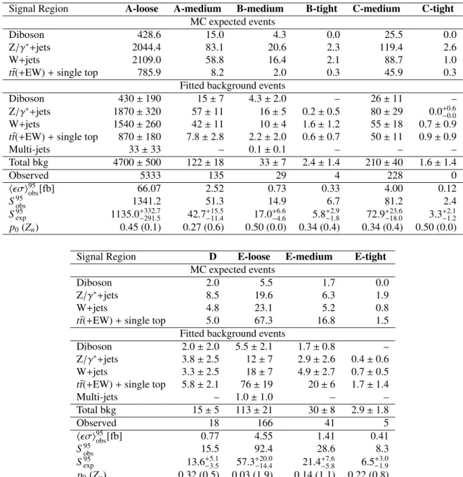
7 Results, Interpretation and Limits

The number of events observed in the data and the number of SM events expected to enter each of the

signal regions, determined using the likelihood fit, are shown in Table 4. Good agreement is observed

between the data and the SM prediction, with no significant excess. The largest observed excess across

the ten SRs, with a p-value for the background-only hypothesis of 0.03, occurs in SR E-loose. Predictions

obtained from the likelihood fits for the numbers of events in the validation regions also agree well

with the observations. Distributions of m

_eff

(incl.) before the final cut on this quantity for data and the

di

ff

erent MC samples normalised with the theoretical cross-sections are shown in Figs. 1–4 for each

of the channels. Examples of typical expected SUSY signals are shown for illustration. These signals

correspond to the processes to which each SR is primarily sensitive – ˜ q q ˜ production for the lower jet

multiplicity SRs (channel A), ˜ q˜

g

associated production for intermediate jet multiplicity SRs (channel B),

and ˜

gg

˜ production for the higher jet multiplicity SRs (channels C, D and E).

Signal Region A-loose A-medium B-medium B-tight C-medium C-tight MC expected events

Diboson 428.6 15.0 4.3 0.0 25.5 0.0

Z/γ^∗+jets 2044.4 83.1 20.6 2.3 119.4 2.6

W+jets 2109.0 58.8 16.4 2.1 88.7 1.0

tt(¯+EW)+single top 785.9 8.2 2.0 0.3 45.9 0.3

Fitted background events

Diboson 430±190 15±7 4.3±2.0 – 26±11 –

Z/γ^∗+jets 1870±320 57±11 16±5 0.2±0.5 80±29 0.0⁺_−0.0^0.6 W+jets 1540±260 42±11 10±4 1.6±1.2 55±18 0.7±0.9 tt(¯+EW)+single top 870±180 7.8±2.8 2.2±2.0 0.6±0.7 50±11 0.9±0.9

Multi-jets 33±33 – 0.1±0.1 – – –

Total bkg 4700±500 122±18 33±7 2.4±1.4 210±40 1.6±1.4

Observed 5333 135 29 4 228 0

hσi⁹⁵_obs[fb] 66.07 2.52 0.73 0.33 4.00 0.12

S⁹⁵_obs 1341.2 51.3 14.9 6.7 81.2 2.4

S⁹⁵_exp 1135.0⁺_−291.5^332.7 42.7⁺_−11.4^15.5 17.0⁺_−4.6^6.6 5.8⁺_−1.8^2.9 72.9⁺_−18.0^23.6 3.3⁺_−1.2^2.1 p0(Zn) 0.45 (0.1) 0.27 (0.6) 0.50 (0.0) 0.34 (0.4) 0.34 (0.4) 0.50 (0.0)

Signal Region D E-loose E-medium E-tight

MC expected events

Diboson 2.0 5.5 1.7 0.0

Z/γ^∗+jets 8.5 19.6 6.3 1.9

W+jets 4.8 23.1 5.2 0.8

t¯t(+EW)+single top 5.0 67.3 16.8 1.5 Fitted background events

Diboson 2.0±2.0 5.5±2.1 1.7±0.8 –

Z/γ^∗+jets 3.8±2.5 12±7 2.9±2.6 0.4±0.6 W+jets 3.3±2.5 18±7 4.9±2.7 0.7±0.5 t¯t(+EW)+single top 5.8±2.1 76±19 20±6 1.7±1.4

Multi-jets – 1.0±1.0 – –

Total bkg 15±5 113±21 30±8 2.9±1.8

Observed 18 166 41 5

hσi⁹⁵_obs[fb] 0.77 4.55 1.41 0.41

S⁹⁵_obs 15.5 92.4 28.6 8.3

S⁹⁵_exp 13.6⁺_−3.5^5.1 57.3⁺_−14.4^20.0 21.4⁺_−5.8^7.6 6.5⁺_−1.9^3.0 p0(Zn) 0.32 (0.5) 0.03 (1.9) 0.14 (1.1) 0.22 (0.8)

Table 4: Numbers of events observed in the signal regions used in the analysis (L

=

20.3 fb

⁻¹

) compared

with background expectations obtained from the fits described in the text. Background uncertainties

include both TF systematics (see Section 6) and CR data statistical uncertainties. No signal contribution

is considered in the CRs for the fit. Empty cells correspond to estimates lower than 0.1 events. Also

shown are 95% CL upper limits on the visible cross-section (

hσi⁹⁵_obs

), the visible number of signal

events (S

⁹⁵_obs

) and the number of signal events (S

⁹⁵_exp

) given the expected number of background events,

as well as

±1σ

excursions on the expectation. The p

₀

-values give the probabilities of the observations

being consistent with the estimated backgrounds and are constrained to

≤

0.5. Also presented are the

equivalent Gaussian significances Z

n

.

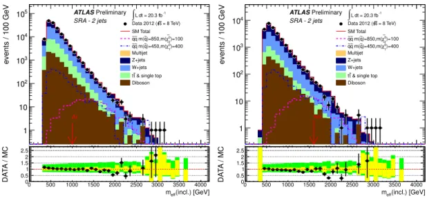
(incl.) [GeV]

meff 0 500 1000 1500 2000 2500 3000 3500 4000

events / 100 GeV

1 10 102

103

104

105 ∫L dt = 20.3 fb^-1

= 8 TeV) s Data 2012 ( SM Total

)=100 0 χ∼1 )=850,m(

q~ m(

q~ q~

)=400 0 χ∼1 )=450,m(

q~ m(

q~ q~ Multijet Z+jets W+jets

& single top t t Diboson Preliminary ATLAS SRA - 2 jets

Al

(incl.) [GeV]

meff

0 500 1000 1500 2000 2500 3000 3500 4000

DATA / MC

0 0.5 1 1.52

2.5 0 500 1000 1500 2000 2500 3000 m3500eff(incl.) [GeV]4000

events / 100 GeV

1 10 102

103

104

L dt = 20.3 fb-1

∫

= 8 TeV) s Data 2012 ( SM Total

)=100 0 χ∼1 )=850,m(

q~ m(

q~ q~

)=400 0 χ∼1 )=450,m(

q~ m(

q~ q~ Multijet Z+jets W+jets

& single top t t Diboson Preliminary ATLAS SRA - 2 jets

Am

(incl.) [GeV]

meff

0 500 1000 1500 2000 2500 3000 3500 4000

DATA / MC

0 0.5 1 1.52 2.5

Figure 1: Observed m

_eff

(incl.) distributions for channel A for ‘loose’ (left) and ‘medium’ (right) selec- tion criteria. With the exception of the multi-jet background (which is estimated using the data-driven technique described in the text), the histograms denote the MC background expectations, normalised to cross-section times integrated luminosity. In the lower panels the yellow error bands denote the experi- mental and MC statistical uncertainties, while the green bands show the total uncertainty. The red arrows indicate the values at which the requirements on m

_eff

(incl.) are applied. Expected distributions for two benchmark model points characterised by ˜ q q ˜ production are also shown for comparison (masses in GeV).

(incl.) [GeV]

meff 0 500 1000 1500 2000 2500 3000 3500 4000

events / 100 GeV

1 10 102

103

104

L dt = 20.3 fb-1

∫

= 8 TeV) s Data 2012 ( SM Total

)=525 0 χ∼1 )=1425,m(

q~ )=1.04 m(× g~ m(

g~ q~

0)=37 χ∼1 )=1612,m(

q~ )=1.04 m(× g~ m(

g~ q~ Multijet Z+jets W+jets

& single top t t Diboson Preliminary ATLAS SRB - 3 jets

Bm

(incl.) [GeV]

meff

0 500 1000 1500 2000 2500 3000 3500 4000

DATA / MC

0 0.5 1 1.5 2

2.5 0 500 1000 1500 2000 2500 3000 m3500_eff(incl.) [GeV]4000

events / 100 GeV

1 10 102

103

L dt = 20.3 fb-1

∫

= 8 TeV) s Data 2012 ( SM Total

)=525 0 χ∼1 )=1425,m(

q~ )=1.04 m(× g~ m(

g~ q~

0)=37 χ∼1 )=1612,m(

q~ )=1.04 m(× g~ m(

g~ q~ Multijet Z+jets W+jets

& single top t t Diboson Preliminary ATLAS SRB - 3 jets

Bt

(incl.) [GeV]

meff

0 500 1000 1500 2000 2500 3000 3500 4000

DATA / MC

0 0.5 1 1.5 2 2.5

Figure 2: Observed m

_eff

(incl.) distributions for channel B for ‘medium’ (left) and ‘tight’ (right) selec-

tion criteria. With the exception of the multi-jet background (which is estimated using the data-driven

technique described in the text), the histograms denote the MC background expectations, normalised to

cross-section times integrated luminosity. In the lower panels the yellow error bands denote the experi-

mental and MC statistical uncertainties, while the green bands show the total uncertainty. The red arrows

indicate the values at which the requirements on m

_eff

(incl.) are applied. Expected distributions for two

benchmark model points characterised by ˜ q˜

g

production are also shown for comparison (masses in GeV).

(incl.) [GeV]

meff 0 500 1000 1500 2000 2500 3000 3500 4000

events / 100 GeV

1 10 102

103

L dt = 20.3 fb-1

∫

= 8 TeV) s Data 2012 ( SM Total

1/2=700

=1000,m CMSSM m0

)=550 0 χ∼1 )=700,m(

g~ m(

g~ g~ Multijet Z+jets W+jets

& single top t t Diboson Preliminary ATLAS SRC - 4 jets

Cm Ct

(incl.) [GeV]

meff

0 500 1000 1500 2000 2500 3000 3500 4000

DATA / MC

0 0.5 1 1.52

2.5 0 500 1000 1500 2000 2500 3000 m3500_eff(incl.) [GeV]4000

events / 100 GeV

1 10 102

103 ∫L dt = 20.3 fb^-1

= 8 TeV) s Data 2012 ( SM Total

)=337 0 χ∼1 )=1162,m(

g~ m(

g~ g~

0)=50 χ∼1 )=1250,m(

g~ m(

g~ g~ Multijet Z+jets W+jets

& single top t t Diboson Preliminary ATLAS SRD - 5 jets

Dt

(incl.) [GeV]

meff

0 500 1000 1500 2000 2500 3000 3500 4000

DATA / MC

0 0.5 1 1.52 2.5

Figure 3: Observed m

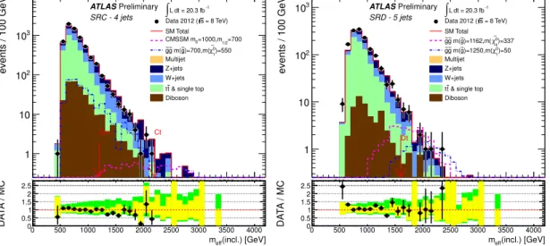
_eff

(incl.) distributions for channels C (left) and D (right). With the exception

of the multi-jet background (which is estimated using the data-driven technique described in the text),

the histograms denote the MC background expectations, normalised to cross-section times integrated

luminosity. In the lower panels the yellow error bands denote the experimental and MC statistical uncer-

tainties, while the green bands show the total uncertainty. The red arrows indicate the values at which

the requirements on m

_eff

(incl.) are applied. Expected distributions for two benchmark model points are

also shown for comparison (masses in GeV).

(incl.) [GeV]

meff

0 500 1000 1500 2000 2500 3000 3500 4000 4500

events / 150 GeV

1 10 102

L dt = 20.3 fb-1

∫

= 8 TeV) s Data 2012 ( SM Total

)=505 0 χ∼1 )=785,m(

± χ∼1 )=1065,m(

g~ m(

g~ g~

)=465 0 χ∼1 )=865,m(

± χ∼1 )=1265,m(

g~ m(

g~ g~ Multijet Z+jets W+jets

& single top t t Diboson Preliminary ATLAS SRE - 6 jets

El

(incl.) [GeV]

meff

0 500 1000 1500 2000 2500 3000 3500 4000 4500

DATA / MC

0 0.5 1 1.5 2

2.5 0 500 1000 1500 2000 2500 3000 3500meff(incl.) [GeV]4000 4500

events / 150 GeV

1 10 102

L dt = 20.3 fb-1

∫

= 8 TeV) s Data 2012 ( SM Total

)=505 0 χ∼1 )=785,m(

± χ∼1 )=1065,m(

g~ m(

g~ g~

)=465 0 χ∼1 )=865,m(

± χ∼1 )=1265,m(

g~ m(

g~ g~ Multijet Z+jets W+jets

& single top t t Diboson Preliminary ATLAS SRE - 6 jets

Em

(incl.) [GeV]

meff

0 500 1000 1500 2000 2500 3000 3500 4000 4500

DATA / MC

0 0.5 1 1.5 2 2.5

(incl.) [GeV]

meff

0 500 1000 1500 2000 2500 3000 3500 4000 4500

events / 150 GeV

1 10

102 -1

L dt = 20.3 fb

∫

= 8 TeV) s Data 2012 ( SM Total

)=505 0 χ∼1 )=785,m(

± χ∼1 )=1065,m(

g~ m(

g~ g~

)=465 0 χ∼1 )=865,m(

± χ∼1 )=1265,m(

g~ m(

g~ g~ Multijet Z+jets W+jets

& single top t t Diboson Preliminary ATLAS SRE - 6 jets

Et

(incl.) [GeV]

meff

0 500 1000 1500 2000 2500 3000 3500 4000 4500

DATA / MC

0 0.5 1 1.5 2 2.5

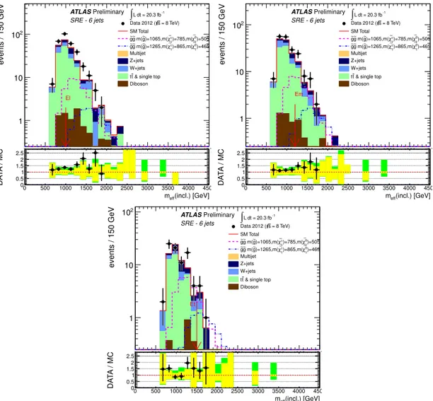
Figure 4: Observed m

_eff

(incl.) distributions for channel E for ‘loose’ (top left), ‘medium’ (top right) and

‘tight’ (bottom) selection criteria. With the exception of the multi-jet background (which is estimated

using the data-driven technique described in the text), the histograms denote the MC background ex-

pectations, normalised to cross-section times integrated luminosity. In the lower panels the yellow error

bands denote the experimental and MC statistical uncertainties, while the green bands show the total

uncertainty. The red arrows indicate the values at which the requirements on m

_eff

(incl.) are applied. Ex-

pected distributions for two benchmark model points characterised by ˜

g˜g

production are also shown for

comparison (masses in GeV).

[GeV]

m0

1000 2000 3000 4000 5000 6000

[GeV]1/2m

300 400 500 600 700 800 900

(1400 GeV) q ~

(1800 GeV) q ~

(2200 GeV) q ~

(1000 GeV) g~

(1200 GeV) g~

(1400 GeV) g~

(1600 GeV) g~

(1800 GeV) g~

H (124 GeV) H (125 GeV) H (126 GeV)

>0 µ

0,

= -2m = 30, A0

β MSUGRA/CMSSM: tan

=8 TeV s

-1, L dt = 20.3 fb

∫

0-lepton combined

ATLAS Preliminary

theory) σSUSY

±1 Observed limit (

exp) σ

±1 Expected limit ( Stau LSP

gluino mass [GeV]

800 1000 1200 1400 1600 1800 2000 2200

squark mass [GeV]

1000 2000 3000 4000 5000

>0 µ

0,

= -2m = 30, A0

β MSUGRA/CMSSM: tan

=8 TeV s

-1, L dt = 20.3 fb

∫

0-lepton combined

ATLASPreliminary

theory) σSUSY

±1 Observed limit (

exp) σ

±1 Expected limit ( Stau LSP

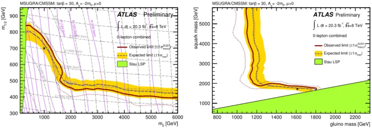
Figure 5: Exclusion limits for MSUGRA

/

CMSSM models with tan

β=

30, A

₀ = −2m0

and

µ >

0 pre- sented (left) in the m

₀

–m

1/2

plane and (right) in the m

_g˜

–m

q_˜

plane. Exclusion limits are obtained by using the signal region with the best expected sensitivity at each point. The blue dashed lines show the expected limits at 95% CL, with the light (yellow) bands indicating the 1σ excursions due to experimental and background-theory uncertainties. Observed limits are indicated by medium (maroon) curves, where the solid contour represents the nominal limit, and the dotted lines are obtained by varying the signal cross- section by the theoretical scale and PDF uncertainties. The black star indicates the MSUGRA/CMSSM benchmark model used in Fig. 3(left).

In the absence of a statistically significant excess limits are set on contributions to the SRs from new physics. Model independent limits are listed in Table 4 for the number of new physics events and the visible cross-section

σ_vis

(defined as the product of the production cross-section times reconstruction efficiency times acceptance), computed assuming an absence of signal in the control regions.

Data from all the channels are used to set limits on SUSY models, taking the SR with the best expected sensitivity at each point in several parameter spaces. A profile log-likelihood ratio test in combination with the CL

s

prescription [68] is used to derive 95% CL exclusion regions. The nominal signal cross-section and the uncertainty are taken from an ensemble of cross-section predictions using di

ff

erent PDF sets and factorisation and renormalisation scales, as described in Ref. [69]. Observed limits are calculated for both the nominal cross-section, and

±1σ

uncertainties. Numbers quoted in the text are evaluated from the observed exclusion limit based on the nominal cross-section less one sigma on the theoretical uncertainty.

In Fig. 5 the results are interpreted in the tan

β=

30, A

₀ =−2m0

,

µ >

0 slice of MSUGRA/CMSSM models

²

. The best performing signal regions are E-tight for m

₀ &

1500 GeV and C-tight for m

₀ .

1500 GeV. Results are presented in both the m

₀

–m

_1/2

and m

_g˜

–m

q_˜

planes. The sparticle mass spectra and decay tables are calculated with SUSY-HIT [70] interfaced to the SOFTSUSY spectrum generator [71] and SDECAY [72].

An interpretation of the results is also presented in Fig. 6 as a 95% CL exclusion region in the (m

g˜,

m

q_˜

)-plane for a simplified set of phenomenological MSSM (Minimal Supersymmetric extension of the SM) models with m

_χ˜0

1

equal to 0, 395 GeV or 695 GeV. In these models the gluino mass and the masses of the ‘light’-flavour squarks (of the first two generations, including both ˜ q

_R

and ˜ q

_L

, and assum- ing mass degeneracy) are set to the values shown on the axes of the figure. All other supersymmetric particles, including the squarks of the third generation, are decoupled.

2Five parameters are needed to specify a particular MSUGRA/CMSSM model: the universal scalar mass,m0, the universal

gaugino massm1/2, the universal trilinear scalar coupling,A0, the ratio of the vacuum expectation values of the two Higgs fields,

tanβ, and the sign of the higgsino mass parameter,µ=±.