Search for direct top squark pair production in final states with one isolated lepton, jets, and missing transverse momentum

A TLAS-CONF-2013-037 26 Mar ch 2013

ATLAS NOTE

ATLAS-CONF-2013-037

March 25, 2013

Search for direct top squark pair production in final states with one isolated lepton, jets, and missing transverse momentum

in √

s = 8 TeV pp collisions using 21 fb ^{− 1} of ATLAS data

The ATLAS Collaboration

Abstract

A search is presented for direct top squark pair production in final states with one isolated electron or muon, jets, and missing transverse momentum in proton-proton collisions at a centre-of-mass energy of 8 TeV. The analysis is based on 20.7 fb ⁻¹ of data collected with the ATLAS detector at the LHC. The top squarks are assumed to decay to a top quark and the lightest supersymmetric particle (LSP) or to a bottom quark and a chargino, where the chargino decays to an on- or off-shell W boson and to the LSP. The data are found to be consistent with Standard Model expectations. Assuming both top squarks decay to a top quark and the LSP, top squark masses between 200 and 610 GeV are excluded at 95%

confidence level for massless LSPs, and top squark masses around 500 GeV are excluded for LSP masses up to 250 GeV. Assuming both top squarks decay to a bottom quark and the lightest chargino, top squark masses up to 410 GeV are excluded for massless LSPs and an assumed chargino mass of 150 GeV.

c Copyright 2013 CERN for the benefit of the ATLAS Collaboration.

Reproduction of this article or parts of it is allowed as specified in the CC-BY-3.0 license.

1 Introduction

The gauge hierarchy problem [1–4] has gained additional attention with the observation of a new particle consistent with the Standard Model (SM) Higgs boson [5, 6] at the LHC [7]. A solution to the hierarchy problem is provided by weak scale supersymmetry (SUSY) [8–16], which extends the SM by introducing supersymmetric partners for all SM particles. If the supersymmetric partner of the top quark (top squark or stop) has a mass below the TeV range, loop diagrams involving top quarks, which are the dominant contribution to the divergence of the Higgs boson mass, can be canceled to a large extent [17, 18]. The superpartners of the left- and right-handed top quarks, ˜t _L and ˜t _R , mix to form the two mass eigenstates

˜t ₁ and ˜t ₂ , where ˜t ₁ is the lighter one. Significant mass-splitting between ˜t ₁ and ˜t ₂ is possible due to the large top Yukawa coupling. A generic R-parity conserving minimal supersymmetric extension of the SM (MSSM) [19–23] predicts the pair production of SUSY particles and the existence of a stable lightest supersymmetric particle (LSP), which can serve as a candidate for dark matter. In a large variety of models, the LSP is the lightest neutralino, ˜ χ ⁰ ₁ , which only interacts weakly and thus escapes detection.

A search is presented for direct ˜t ₁ pair production, extending the analysis presented in Ref. [24]. In addition to using the full 2012 data set (20.7 fb ^{− 1} ), the signal selections have been improved and a new shape-fit approach has been developed. Two simplified ˜t ₁ decay scenarios are considered in this note:

either each ˜t ₁ decays to a top quark and the LSP (˜t ₁ → t + χ ˜ ⁰ ₁ ), or each ˜t ₁ decays to a bottom quark and the lightest chargino (˜t ₁ → b + χ ˜ ^± ₁ ), where the ˜ χ ^± ₁ ’s are the mass eigenstates formed from the linear superposition of the SUSY partners of the Higgs and electroweak gauge bosons and decay to the LSP ˜ χ ⁰ ₁ via an on- or off-shell W boson ( ˜ χ ^± ₁ → W ^{( ∗ )} + χ ˜ ⁰ ₁ ). Depending on the assumptions on the SUSY particle masses and the choice of mixing parameters for the neutralinos and top squarks, one of these two decay modes can be dominant.

The final state for the ˜t ₁ → t + χ ˜ ⁰ ₁ signal scenario is characterised by a top-antitop quark pair (t¯t) produced in association with possibly large missing transverse momentum (the magnitude of which is referred to as E _T ^miss ) from the two undetected LSPs. The final state for the ˜t ₁ → b + χ ˜ ^± ₁ signal scenario is similar: it contains two virtual or real W bosons, two jets originating from a b-quark (b-jets) and two LSPs, but the presence of ˜ χ ^± ₁ ’s in the decay chain alters the kinematic properties with respect to the

˜t ₁ → t + χ ˜ ⁰ ₁ decay.

Searches for direct stop pair production have been previously reported by the ATLAS [24–33] and CMS [34–37] collaborations, as well as by the CDF and DØ collaborationss assuming different SUSY mass spectra and decay modes (see for example Refs. [38, 39]). Searches for stops via gluino pair (˜ g g) ˜ production have been reported by the ATLAS [40–43] and CMS [44–48] collaborations.

The present search is performed with the ATLAS detector [49]. The magnetic system consists of a central solenoid, and an air-core barrel toroid and two endcap toroidal magnets supporting the muon spectrometer. The inner tracking detector (ID), placed inside the solenoid, consists of silicon pixel, sili- con microstrip, and transition radiation detectors and provides precision tracking of charged particles for pseudorapidity | η | < 2.5 ¹ . The calorimeter placed outside the solenoid covers | η | < 4.9 and is composed of sampling electromagnetic and hadronic calorimeters with either liquid argon (LAr) or scintillating tiles as the active media. The muon spectrometer surrounds the calorimeters and consists of a system of precision tracking chambers in | η | < 2.7, and detectors for triggering in | η | < 2.4.

The analysis is based on data recorded by the ATLAS detector in 2012 corresponding to 20.7 fb ^{− 1} of integrated luminosity with the LHC operating at a pp centre-of-mass energy of 8 TeV. The data were collected requiring either a single-lepton (electron or muon) or an E _T ^miss trigger. The combined trigger

1

ATLAS uses a right-handed coordinate system with its origin at the nominal interaction point in the centre of the detector

and the z-axis along the beam pipe. Cylindrical coordinates (r, φ) are used in the transverse plane, φ being the azimuthal

angle around the beam pipe. The pseudorapidity η is defined in terms of the polar angle θ by η = − ln tan(θ/2), and ∆R =

p (∆η)

+ (∆φ)

efficiency is >98% for the lepton and E ^miss _T selection criteria applied in this analysis. Requirements that ensure the quality of beam conditions, detector performance, and data are imposed.

2 Signal and Background Simulation

Monte Carlo (MC) simulation samples are used to aid in the description of the background and to model the SUSY signal. The MC samples are processed either with a full ATLAS detector simulation [50]

based on the Geant4 program [51] or a fast simulation based on the parameterization of the response of the electromagnetic and hadronic showers in the ATLAS calorimeters [52]. The effect of multiple pp interactions in the same or nearby bunch crossing is also simulated. Production of top quark pairs is simulated with PowHeg [53–55]. AcerMC [56] samples with various parameter settings are used to assess the uncertainties associated with initial and final state radiation (ISR/FSR). The parameter settings for the ISR/FSR variations have been obtained from a dedicated data study [57]. The ALPGEN [58] generator is employed to assess the t¯t modelling uncertainty. A top quark mass of 172.5 GeV is used consistently.

W and Z /γ ^∗ production in association with jets are each modelled with SHERPA [59]. Diboson VV (WW, WZ, ZZ) production is simulated with ALPGEN with up to three additional partons. Single top quark production is modelled with MC@NLO (s-channel and Wt-channel) [60, 61] and AcerMC (t-channel). The production of t¯t in association with Z or W (t¯t + V) is generated with MADGRAPH [62]. The t¯t + V mod- elling uncertainty is assessed using the ALPGEN generator. For the event generation next-to-leading order (NLO) PDFs CT10 [63] are used with all NLO MC samples and with SHERPA. For all other samples LO PDFs, namely CTEQ6L1 [64], are used. Fragmentation and hadronization for all samples are performed with PYTHIA [65], except for single top samples where MC@NLO is used with HERWIG and JIMMY [66]

for the underlying event. The t¯t, single top and t¯t + V production cross-sections are normalized to approximate next-to-next-to-leading order (NNLO) [67], next-to-next-to-leading-logarithmic accuracy (NLO+NNLL) [68–70] and NLO [71, 72] calculations, respectively. The theoretical cross-sections for W+jets and Z+jets are calculated with DYNNLO [73] with the MSTW 2008 NNLO [74] PDF set. The theoretical t¯t and W +jets cross-sections are only used for illustrative purposes, while the final results are normalized using data. Expected diboson yields are normalized using NLO QCD predictions obtained with MCFM [75, 76].

For high jet multiplicities the description of data is improved by reweighting the PowHeg t¯t sample to match the jet multiplicity distribution of ALPGEN, while keeping the overall normalization invariant.

Furthermore, the data modelling of W +jets production is improved by reweighting the SHERPA heavy- flavour quark p _T distribution to match that of ALPGEN.

Stop pair production with ˜t ₁ → t + χ ˜ ⁰ ₁ is modelled using HERWIG++ [77]. A signal grid is generated with a step size of at most 50 GeV (with smaller step sizes towards the region of m _˜t

1

& m _t + m _{χ ˜}

1

) both for the stop and LSP mass values. The ˜t ₁ is chosen to be mostly the partner of the right-handed top quark (the ˜t _R component is about 70%) ² , and the ˜ χ ⁰ ₁ to be almost a pure bino. Different hypotheses on the nature of the left/right mixing in the stop sector and the bino-like neutralino might lead to different acceptance values. A subset of purely ˜t _L models is generated, varying the stop mass, while fixing the ˜ χ ⁰ ₁ mass to assess the variation in acceptance and hence sensitivity. In addition, a selection of signal models with various stop masses is generated with the MADGRAPH event generator. The results are found to be consistent with HERWIG++ within the statistical precision of the samples.

Stop pair production with ˜t ₁ → b + χ ˜ ^± ₁ is modelled using MADGRAPH and PYTHIA. Two signal grids with different assumptions about the chargino-LSP mass difference are considered. In both signal grids the stop and LSP masses are varied. The first signal grid fixes the chargino mass to two times the mass of the LSP (m _{χ ˜}

1

= 2 × m _{χ ˜}

1

), motivated by the pattern in GUT-scale models with gaugino universality.

2

The stop mixing matrix is set with diagonal entries of 0.55 and off-diagonal entries of ± 0.83.

2

In the second signal grid m χ _˜

= 150 GeV is fixed to be well above the present chargino mass limit from LEP [78]. In the MSSM, the ˜t ₁ → b + χ ˜ ^± ₁ branching ratio might not reach 100%, as assumed in the simplified model, if ˜t ₁ → t + χ ˜ ⁰ ₁ / χ ˜ ⁰ ₂ decays are kinematically allowed, but high branching ratios can occur in the allowed parameter space. Depending on the left/right nature of the ˜t ₁ and the higgsino/bino mixture in the neutralino sector, the b + χ ˜ ^± ₁ mode may still be dominant.

Signal cross-sections are calculated to NLO, including the resummation of soft gluon emission at next-to-leading-logarithmic accuracy (NLO+NLL) [79–81]. The nominal cross-section and the uncer- tainty are taken from an envelope of cross-section predictions using different PDF sets and factorization and renormalization scales, as described in Ref. [82]. ISR specific uncertainties for the signal mod- elling are not included, but expected to be smaller than the theoretical uncertainty on the signal, given the presence of real E _T ^miss in the stop decay. The ˜t ₁ pair production cross-section is (5.6 ± 0.8) pb for m _˜t

1

= 250 GeV, and (0.025 ± 0.004) pb for m _˜t

1

= 600 GeV.

3 Event Selection and Reconstruction

Events must pass basic quality criteria to reject detector noise and non-collision backgrounds [83,84] and are required to have at least one reconstructed primary vertex [85] associated with five or more tracks with transverse momentum p _T > 0.4 GeV. Events are retained if they contain exactly one muon [86]

with | η | < 2.4 and p T > 25 GeV or one electron passing ‘tight’ [87] selection criteria with | η | < 2.47 and p _T > 25 GeV. Leptons are required to be isolated from other particles. The scalar sum of the transverse momenta of tracks above 1 GeV within a cone of size ∆R < 0.2 around the lepton candidate is required to be < 10% of the electron p T , and required to be < 1.8 GeV for a muon. Events are rejected if they contain additional electrons or muons passing looser selection criteria and have p _T >

10 GeV. Jets are reconstructed from three-dimensional calorimeter energy clusters using the anti-k t jet clustering algorithm [88, 89] with a distance parameter of 0.4. Jet energies are corrected [83] for detector inhomogeneities, the non-compensating nature of the calorimeter, and the impact of multiple overlapping pp interactions, using factors derived from test beam, cosmic ray, pp collision data and from the detailed Geant4 detector simulation. Events with four or more jets are selected where the jets must satisfy

| η | < 2.5 and p _T > 80, 60, 40, 25 GeV, respectively. Jets containing a b-hadron decay are identified using the ‘MV1’ b-tagging algorithm [90–93], which exploits both impact parameter and secondary vertex information. An operating point corresponding to an average 75% b-tagging efficiency and a < 2%

misidentification rate, obtained for light-quark/gluon jets for jets with p _T > 20 GeV and | η | < 2.5 in t¯t MC events, is employed. At least one of the leading four jets needs to be identified as a b-jet.

To resolve overlaps between reconstructed jets and electrons, jets within a distance of ∆R < 0.2 of an electron candidate are rejected. Furthermore, any lepton candidate with a distance ∆R < 0.4 to the closest remaining jet is discarded. The measurement of E _T ^miss is based on the transverse momenta of all electron and muon candidates, all jets after overlap removal, and all calorimeter energy clusters not associated to such objects.

3.1 Signal Selections

Six signal regions (SRs) are defined in order to optimize the sensitivity for different stop and LSP masses, as well as the two considered stop decay scenarios. Three signal regions (labeled SRbC 1–3, where “bC”

is a moniker for “b+Chargino”) have been optimized for the ˜t ₁ → b+ χ ˜ ^± ₁ decay scenario, where increasing

label numbers correspond to increasingly stricter event selection criteria. The loosest selection, SRbC1,

has been retained from the previous analysis [24]. It is most sensitive for signal models with medium

stop masses (about 200–400 GeV) and medium to large chargino masses (about 100–300 GeV). The

two tighter selections, SRbC2/3, have been designed for signal models with high stop masses (about

350–500 GeV) and medium-to-high mass differences between the stop and chargino (& 150 GeV). In such models, the two b-quarks have significantly larger momentum than in the main t¯t background.

Consequently, two or more b-jets are required in these signal regions, each with large p T .

Three signal regions (labeled SRtN 1–3, where “tN” is a moniker for “t+Neutralino”) have been optimized for the ˜t ₁ → t + χ ˜ ⁰ ₁ decay scenario, where increasing label numbers correspond to increasingly stricter event selection criteria. The loosest selection, SRtN1 shape, exploits a multi-binned shape fit, described in more detail below, that targets the challenging stop model parameter space where the stop and its decay products are nearly mass degenerate (m _˜t

1

& m t + m _{χ ˜}

1

). The SRtN2 selection has been retained from the previous analysis [24], and it is the most sensitive selection for models with large LSP masses. The tightest selection, SRtN3, is designed for models with large stop masses.

The dominant background in all signal regions arises from dileptonic t¯t events in which one of the leptons is not identified, is outside the detector acceptance, or is a hadronically decaying τ lepton. In all these cases, the t¯t decay products include two or more high-p _T neutrinos, resulting in large E ^miss _T and large transverse mass ³ m T .

All three SRtN selections impose a requirement on the 3-jet mass m _{j j j} of the hadronically decaying top quark to specifically reject the t¯t background where both W bosons from the top quarks decay lepton- ically. The jet-jet pair with an invariant mass above 60 GeV which has the smallest ∆R is selected to form the hadronic W boson. The mass m _{j j j} is reconstructed from the third jet closest in ∆R to the hadronic W boson momentum vector and 130 GeV < m _{j j j} < 205 GeV is required.

There is no m j j j requirement in the SRbC 1–3 event selections since these target ˜t ₁ → b+ χ ˜ ^± ₁ scenarios where no intermediate top quark appears in the decays. To reduce background from dileptonic t¯t events with a hadronic τ in the final state, the SRbC 1–3 selections veto events that contain an isolated track with p T > 10 GeV which passes basic track quality criteria and does not match the selected lepton.

The isolation criterion requires no additional track with p T > 3 GeV in a cone of ∆R < 0.4 around the candidate track.

For increasing stop mass and increasing mass difference between the stop and the LSP the require- ments are tightened on E _T ^miss , on the ratio E ^miss _T / √

H _T , where H _T is the scalar sum of the momenta of the four selected jets, and on m _T . In addition, for the signal regions SRbC2 and SRbC3 requirements on the effective mass, m eff , defined as sum of the transverse momenta of all jets with p T > 30 GeV, the transverse momentum of the charged lepton and E _T ^miss , and of the transverse momenta of the two leading b-jets are imposed.

Additionally, requirements are tightened on two variants of the variable m T 2 [94], a generalization of the transverse mass applied to signatures with two undetected particles, to further reduce the dileptonic t¯t background. For an event characterized by two one-step decay chains, a and b, each producing a missing particle C, the m T 2 value of the event is defined by the minimization over all possible 2-momenta,

~ p T a , ~ p T b , such that their sum gives the observed missing transverse momentum ~ p _T ^miss : m _{T 2} ≡ min

~ p

+~ p

=~ p

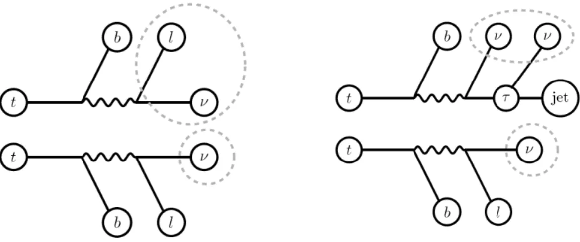
{ max(m _{T a} , m _{T b} ) } , (1) where m _{T i} is the transverse mass of branch i for a given hypothetical allocation (~ p _{T a} ^C , ~ p _{T b} ^C ) of the missing particle momenta. Note that there is an implicit use of an input mass for the missing particles when computing m _{T i} . The choice for this input mass is arbitrary, since for a given choice there is a known relationship between the mass of the parent particles and the endpoint of m _{T 2} . The definition in Eq. 1 can be easily extended to more general decay chains. Figure 1 illustrates two such generalizations. The first is a form of asymmetric m _{T 2} (am _{T 2} ) [95–97] in which the missing particle is the W boson for the branch with the lost lepton and the neutrino is the missing particle for the branch with the observed charged

3

The transverse mass is defined as m

= 2p

E

(1 − cos(∆φ)), where ∆φ is the azimuthal angle between the lepton and missing transverse momentum direction.

4

Figure 1: Illustration of the am _{T 2} (left) and m ^τ _{T 2} (right) variables used to discriminate against dileptonic t¯t background where one lepton is lost (left) or decays into a hadronically decaying τ (right). The dashed lines indicate what objects are ‘missing’ to define the phase space for the minimization in Eq. 1.

lepton. For dileptonic t¯t events with a lost lepton, the input masses are chosen such that am T 2 is bounded by the top quark mass, whereas for new physics it can exceed this bound. The required input masses are m ν for the branch with the visible lepton and m W for the other branch. The second m T 2 variant (m ^τ _{T 2} ) is designed for events with a hadronic τ lepton by using the W bosons as parent particles and the ‘τ-jet’ as a visible particle on one branch and the observed lepton for the other branch. The input masses are then picked to be zero so that the hadronic-τ t¯t background has an endpoint around the W boson mass in the limit of a massless τ.

Furthermore, requirements on a minimal azimuthal (transverse) separation between the leading or sub-leading jet and the missing transverse momentum direction (∆ϕ(jet _1,2 , ~ p _T ^miss )) are used to suppress backgrounds from mostly multijet events with mismeasured E ^miss _T . Table 1 gives an overview of the signal region requirements and the resulting product of the acceptance and reconstruction efficiency for selected benchmark points. The numbers of observed events in each of the signal regions after applying all selection criteria are given in Tables 2 through 4.

The SRtN1 shape interpretation differs from the other signal regions as follows. While the other

selections are based on a single-bin signal region, the SRtN1 shape probes a potential signal in several

signal-sensitive bins spanned by the E ^miss _T and m T variables. This strategy exploits (binned) shape infor-

mation to improve the sensitivity. The approach is particularly useful for the challenging stop models,

where due to a small mass difference between the stop and its decay products, the kinematic variables

(e.g. E ^miss _T m T , etc.) resemble those of the t¯t background to a large extent. The binning defined for

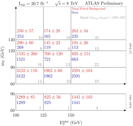
SRtN1 shape is illustrated in Figure 2. In the E ^miss _T and m _T variables a 3 × 4 matrix is defined, with the

default ≥ 1 b-jet requirement. These 12 bins serve both to probe a signal and to normalize the t¯t back-

ground. For completeness, also the additional three bins with a b-jet veto are shown in Figure 2, which

are dominated by W +jets events. The full SRtN1 shape event selection, as listed in Table 1, is applied

before events are sorted into the 15 bins, except for the b-jet requirement which is used as a veto for the

three bins dedicated to the W+jets normalization. All events which pass the SRtN1 shape event selection

fall into exactly one of the bins, i.e. the bins are mutually exclusive. The bins for E ^miss _T > 150 GeV or

for m _T > 140 GeV are defined without upper boundaries, in E ^miss _T and m _T respectively.

Requirement SRtN1 shape SRtN2 SRtN3 SRbC1 SRbC2 SRbC3

∆ϕ(jet ₁ , ~ p _T ^miss ) > 0.8 - 0.8 0.8 0.8 0.8

∆ϕ(jet ₂ , ~ p _T ^miss ) > 0.8 0.8 0.8 0.8 0.8 0.8

E _T ^miss [GeV] > 100 ^(⋆) 200 275 150 160 160

E _T ^miss / √

H _T [GeV ^1/2 ] > 5 13 11 7 8 8

m _T [GeV] > 60 ^(⋆) 140 200 120 120 120

m eff [GeV] > - - - - 550 700

am _{T 2} [GeV] > - 170 175 - 175 200

m ^τ _{T 2} [GeV] > - - 80 - - -

m j j j Yes Yes Yes - - -

N ^{iso − trk} = 0 - - - Yes Yes Yes

Number of b-jets ≥ 1 1 1 1 2 2

p T (leading b-jet) [GeV] > 25 25 25 25 100 120

p _T (second b-jet) [GeV] > - - - - 50 90

A × ε benchmark points (masses in GeV)

m(˜t , LSP) = 225, 25 5.2 × 10 ^{− 3} 1.0 × 10 ^{− 5} 4.2 × 10 ^{− 6} 5.7 × 10 ^{− 4} 3.1 × 10 ^{− 5} 1.1 × 10 ^{− 5} m(˜t , LSP) = 350, 150 1.2 × 10 ^{− 2} 1.2 × 10 ^{− 4} 3.0 × 10 ^{− 5} 4.1 × 10 ^{− 3} 2.3 × 10 ^{− 4} 5.7 × 10 ^{− 5} m(˜t , LSP) = 500, 200 4.1 × 10 ^{− 2} 8.4 × 10 ^{− 3} 3.8 × 10 ^{− 3} 3.1 × 10 ^{− 2} 6.0 × 10 ^{− 3} 1.6 × 10 ^{− 3} m(˜t , LSP) = 600, 50 5.9 × 10 ^{− 2} 2.7 × 10 ^{− 2} 2.3 × 10 ^{− 2} 5.7 × 10 ^{− 2} 1.7 × 10 ^{− 2} 8.4 × 10 ^{− 3} m(˜t , χ ^± ₁ , χ ⁰ ₁ ) = 200, 150, 75 2.4 × 10 ^{− 3} 6.2 × 10 ^{− 6} 5.1 × 10 ^{− 6} 6.1 × 10 ^{− 4} 2.0 × 10 ^{− 5} 8.2 × 10 ^{− 6} m(˜t , χ ^± ₁ , χ ⁰ ₁ ) = 350, 200, 100 2.5 × 10 ^{− 2} 3.9 × 10 ^{− 4} 1.5 × 10 ^{− 4} 9.9 × 10 ^{− 3} 2.3 × 10 ^{− 3} 6.6 × 10 ^{− 4} m(˜t , χ ^± ₁ , χ ⁰ ₁ ) = 600, 300, 150 3.8 × 10 ^{− 2} 5.0 × 10 ^{− 3} 2.3 × 10 ^{− 3} 5.1 × 10 ^{− 2} 2.4 × 10 ^{− 2} 1.8 × 10 ^{− 2}

(⋆)

: The signal region SRtN1 shape uses bins spanned by the E

and m

variables, as described in the text.

Table 1: Selection requirements defining the signal regions. The bottom part lists the expected acceptance times efficiency for selected signal benchmark models.

3.2 Background Modelling

The leading and sub-leading backgrounds arise from t¯t and W+jets production, respectively. They are estimated using dedicated control regions, making the analysis more robust against MC mis-modelling effects.

With the exception of SRtN1 shape, for each signal region two control regions (CRs) enriched in either t¯t events (TCR) or W+jets events (WCR) are defined to normalize the corresponding backgrounds using data. Both control regions differ from the associated signal region by the m _T requirement which is set to 60 GeV < m T < 90 GeV for the control region. The W+jets control region also has, in addi- tion to the aforementioned m _T requirement, a b-jet veto instead of a b-jet requirement to reduce the t¯t contamination. Moreover, the requirements on E ^miss _T , am T 2 are slightly loosened by 20 − 25 GeV and the requirement on m ^τ _{T 2} is dropped to increase the statistics, where needed. All the other signal region requirements are unchanged in the corresponding control regions. Top pair production accounts for 60–

80% of events in the top control regions and W +jets production for 70–90% in the W control regions.

6

100 125 150 60

90 120 140

60 90

E ^miss _T (GeV) m T (G eV)

L _int = 20 . 7 fb ^{− 1} √

s = 8 TeV ATLAS Preliminary

≥ 1 b -j et b-jet v eto

Total Fitted Background Data

Signal (m

, m

) = (350, 150)

1289 ± 85 825 ± 56 1441 ± 103 3122 ± 116 1962 ± 60 2591 ± 104 1535 ± 260 760 ± 120 695 ± 151

290 ± 60 145 ± 23 101 ± 26 250 ± 57 174 ± 28 262 ± 34

1289 825 1441

3122 1962 2591

1521 721 663

268 119 113

253 165 235

1 1 4

14 10 19

16 13 22

8 8 15

16 18 41

Figure 2: Schematic illustration of the shape-fit binning as used in SRtN1 shape. The E _T ^miss and m T

variables are used to define a matrix of 3 × 4 bins (top part). These 12 bins are sensitive to stop models while also being enriched with t¯t background. An additional three bins are defined (bottom part) with a b-veto, leading to W+jets events as the dominant contribution. The numbers of background events as shown are obtained from a fit to the six t¯t and W+jets enriched bins with 60 GeV < m _T < 90 GeV (c.f.

Sections 3.2 and 5).

The maximum signal contamination, for all signal grid points studied, is 10% for the ˜t ₁ → t + χ ˜ ⁰ ₁ control regions and 8% for the ˜t ₁ → b + χ ˜ ^± ₁ control regions.

The t¯t yields fitted in the control regions are validated in dedicated top validation regions (TVR) that differ from the control region in their m _T requirement, which is 90 GeV < m _T < 120 GeV for the latter.

There is thus no event overlap with the associated signal region nor control regions.

For each signal region, a simultaneous likelihood fit to the signal region and the two associated control regions is performed to normalize the t¯t and W +jets background estimates and to determine or limit a potential signal contribution. The fit can also be configured to use only the control regions, to validate the MC/data agreement for the background when the normalization factors and uncertainties are extrapolated to the signal regions.

For the SRtN1 shape selection, the t¯t and W+jets backgrounds, together with a potential signal con-

tribution, are simultaneously fitted in 15 mutually exclusive bins (c.f. Figure 2). In order to minimize

the MC dependence on the E _T ^miss modelling, the t¯t and W +jets backgrounds are separately normalised in

each E ^miss _T slice. Thus, there are three t¯t and three W +jets normalization parameters, which are applied

to all m T bins in the given E ^miss _T range. This approach increases the robustness of the fit against MC

mis-modelling at the expense of a reduced statistical precision.

The remaining backgrounds are determined in the same way for all regions. The multijet background, which mainly originates from jets misidentified as leptons, is estimated using the matrix method [98] and is found to be negligible. Other background contributions (VV, t¯t+ V, single top) are estimated using MC simulation normalized to the theoretical cross-sections, as described in Section 2. The Z+jets background is found to be negligible in all signal regions and control regions.

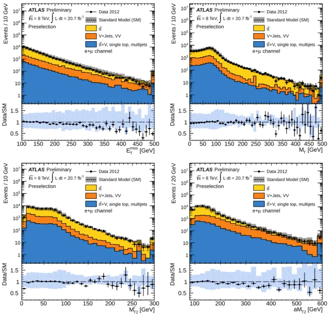
Good agreement between data and SM predictions before the fit is found in all relevant distributions for the preselection common to all signal regions, as shown for E ^miss _T , m _T , m ^τ _{T 2} and am _{T 2} in Figure 3. As the background prediction is measured from control regions with the same or very similar requirements on E ^miss _T as the signal regions, the slight disagreement in the E _T ^miss distribution visible in Figure 3 has a negligible impact on the final result. The same is true by construction for any other variable other than m T . Figure 4 shows the distribution of kinematic variables used to define the signal regions for SM backgrounds and two characteristic signal models after applying all signal selection requirements except that one on the variable shown.

4 Systematic Uncertainties

Since the normalization of the dominant backgrounds, t¯t and W +jets, is obtained from control regions, the theoretical and modelling uncertainties that introduce a difference in acceptance between the control regions and the signal regions are dominating. In case of the shape fit, the uncertainties are evaluated for all bins.

For t¯t the theoretical uncertainties are evaluated by comparing different event generators (PowHeg, before reweighting, and ALPGEN), parton shower modelling (PYTHIA and HERWIG), by varying ISR/FSR and QCD scale parameters. Together with a small uncertainty on the acceptance from the choice of the PDF set, these uncertainties account for 7–42% uncertainties on the transfer factors from the control to the signal regions

For the W+jets background, the theoretical and MC modelling uncertainties are estimated by compar- ing the event generators SHERPA and ALPGEN and are found to be of the order of 25% for the extrapolation from events with no b-jet to events with at least one b-jet and an additional 5–20% for the extrapolation in the variables differing between control region and signal region. Based on the recent measurement of the W + b-jet cross-section from ATLAS [99] and the extrapolation of the uncertainties to higher jet mul- tiplicites, an additional uncertainty of 28% is assigned to the W +heavy-flavour component to describe its relative cross-section uncertainty with respect to the inclusive W +jets background.

Electroweak single top production is associated with an 8% theoretical cross-section uncertainty [68–

70]. For the acceptance, twice the uncertainty of the t¯t background is assumed. The total uncertainty on the t¯t + V background is 44%, which is due to a combination of a 30% uncertainty on the cross-section and scale choices, a 30% uncertainty on the generator modelling from a comparison of ALPGEN and MADGRAPH, and an additional 10% uncertainty on the influence of the availability of a finite number of partons from the modelling. The uncertainty on the multijet background is based on the matrix method, with an uncertainty of 70%, estimated from the ratio of the tight/loose lepton efficiencies. A conservative uncertainty of 100%, derived from a comparison from different MC generators, is assigned to the diboson and Z+jets background estimates.

Experimental uncertainties affect the signal and background yields estimated from MC events and are dominated by the uncertainties in jet energy scale, jet energy resolution, b-tagging, and modelling of multiple pp interactions. Uncertainties related to the trigger and lepton reconstruction and identification (momentum and energy scales, resolutions and efficiencies) give smaller contributions. The uncertainty on the integrated luminosity of 3.6% is derived, following the same methodology as that detailed in [100], from a preliminary calibration of the luminosity scale derived from beam-separation scans performed in

8

Events / 10 GeV

1 10 102

103

104

105

106

107 Data 2012

Standard Model (SM) t

t V+Jets, VV

+V, single top, multijets t

t L dt = 20.7 fb-1

∫

= 8 TeV, s

channel µ e+

Preliminary ATLAS

Preselection

[GeV]

T

E

100 150 200 250 300 350 400 450 500

Data/SM

0.5 1 1.5

Events / 10 GeV

1 10 102

103

104

105

106

107

Data 2012 Standard Model (SM)

t t V+Jets, VV

+V, single top, multijets t

t L dt = 20.7 fb-1

∫

= 8 TeV, s

channel µ e+

Preliminary ATLAS

Preselection

[GeV]

M

0 50 100 150 200 250 300 350 400 450 500

Data/SM

0.5 1 1.5

Events / 10 GeV

1 10 102

103

104

105

106

107 _{Data 2012}

Standard Model (SM) t

t V+Jets, VV

+V, single top, multijets t

t L dt = 20.7 fb-1

∫

= 8 TeV, s

channel µ e+

Preliminary ATLAS

Preselection

[GeV]

T2

M

0 50 100 150 200 250 300

Data/SM

0.5 1 1.5

Events / 20 GeV

1 10 102

103

104

105

106

107 Data 2012

Standard Model (SM) t

t V+Jets, VV

+V, single top, multijets t

t L dt = 20.7 fb-1

∫

= 8 TeV, s

channel µ e+

Preliminary ATLAS

Preselection

[GeV]

aM

100 200 300 400 500 600

Data/SM

0.5 1 1.5

Figure 3: Comparison of data with MC predictions at the preselection stage, which consists of the stan-

dard trigger, data quality, lepton, ≥ 4 jets (p _T > 80, 60, 40, 25 GeV, respectively), and E ^miss _T > 100 GeV

requirements as well as the requirement of at least one b-tagged jet. The top row shows the E _T ^miss and the

m T distributions, while the bottom row shows the two variants of m T 2 : m ^τ _{T 2} and am T 2 . All plots show

the combined electron and muon channels, using nominal cross-sections, as described in Section 2. The

last bin includes the content of the overflow bin. Hatched areas indicate the combined MC statistical, jet

energy scale and jet energy resolution uncertainty.

Events / 50 GeV

10-1

1 10 102

103

104

105

106

107

108

Data 2012 Standard Model (SM)

t t V+Jets, VV

+V, single top, multijets t

t = 25 [GeV]

χ0

= 225, m

~t m

= 150 [GeV]

χ0

= 350, m

~t m

L dt = 20.7 fb-1

∫

= 8 TeV, s

channel µ e+

Preliminary ATLAS

SRtN1 shape

[GeV]

M

0 50 100 150 200 250 300 350 400 450 500

Data/SM

0 1 2

Events / 50 GeV

10-1

1 10 102

103

104

105

Data 2012 Standard Model (SM)

t t V+Jets, VV

+V, single top, multijets t

t = 200 [GeV]

χ0

= 500, m

~t m

= 50 [GeV]

χ0

= 600, m

~t m

L dt = 20.7 fb-1

∫

= 8 TeV, s

channel µ e+

Preliminary ATLAS

SRtN2

[GeV]

T

E

200 250 300 350 400 450 500 550 600 650

Data/SM

0 1 2

Events / 50 GeV

10-1

1 10 102

103

104

105

Data 2012 Standard Model (SM)

t t V+Jets, VV

+V, single top, multijets t

t = 200 [GeV]

χ0

= 500, m

~t m

= 50 [GeV]

χ0

= 650, m

~t m

L dt = 20.7 fb-1

∫

= 8 TeV, s

channel µ e+

Preliminary ATLAS

SRtN3

[GeV]

T2

M

0 50 100 150 200 250 300 350 400 450 500

Data/SM

0 1 2

1/2Events / 4 GeV

10-1

1 10 102

103

104

105

106 ^{Data 2012}

Standard Model (SM) t

t V+Jets, VV

+V, single top, multijets t

t = 75 [GeV]

χ0

= 150, m

χ±

= 200, m

t~

m

= 100 [GeV]

χ0

= 200, m

χ±

= 350, m

t~

m

L dt = 20.7 fb-1

∫

= 8 TeV, s

channel µ e+

Preliminary ATLAS

SRbC1

1/2

] [GeV H

/ E

0 5 10 15 20 25 30 35 40

Data/SM

0 1 2

Events / 50 GeV

10-1

1 10 102

103

104

105 ^{Data 2012}

Standard Model (SM) t

t V+Jets, VV

+V, single top, multijets t

t = 100 [GeV]

χ0

= 200, m

χ±

= 350, m

~t

m

= 150 [GeV]

χ0

= 300, m

χ±

= 600, m

~t

m

L dt = 20.7 fb-1

∫

= 8 TeV, s

channel µ e+

Preliminary ATLAS

SRbC2

[GeV]

aM

50 100 150 200 250 300 350 400 450 500

Data/SM

0 1 2

Events / 200 GeV

10-1

1 10 102

103

104 ^{Data 2012}

Standard Model (SM) t

t V+Jets, VV

+V, single top, multijets t

t = 100 [GeV]

χ0

= 200, m

χ±

= 350, m

t~

m

= 150 [GeV]

χ0

= 300, m

χ±

= 600, m

t~

m

L dt = 20.7 fb-1

∫

= 8 TeV, s

channel µ e+

Preliminary ATLAS

SRbC3

[GeV]

m

500 1000 1500 2000 2500

Data/SM

0 1 2

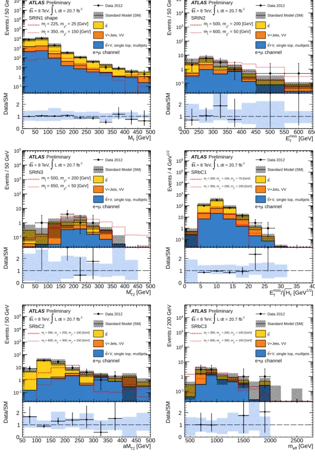
Figure 4: For each signal region one characteristic distribution is shown, with the full event selection of the signal region applied, except for the requirement on the shown quantity. The distribution of m _T (top left) is shown for the selection of the shape fit, before dividing into different bins of E _T ^miss . All plots show the combined electron and muon channels, using nominal cross-sections, as described in Section 2.

Two selected signal model distributions are shown, which are in the expected sensitivity reach of a given signal region. The last bin includes the content of the overflow bin. Hatched areas indicate the combined MC statistical, jet energy scale and jet energy resolution uncertainty.

10

April 2012. Additional sub-dominant uncertainties are due to the limited statistics of the SM MC samples and of the data in the control regions. Systematic uncertainties due to the isolated track veto have been studied, including its dependence on multiple pp interactions in one bunch crossing.

All systematic uncertainties are treated as nuisance parameters with Gaussian shapes in a fit based on the profile likelihood method [101].

5 Results

A set of SM background predictions that is independent of the observation in the signal regions is ob- tained from a fit to the control regions only ⁴ . Background predictions in the signal and validation regions are computed from the background yields fitted to the control regions using appropriate transfer factors obtained from simulation. Tables 2, 3, and 4 list the results of these fits for the dominant SM background sources together with observed event counts for the control, validation and signal regions. The predicted numbers of t¯t and W +jets events using nominal cross-sections as described in Section 2 are listed in parentheses, and are compatible with the fitted background predictions within uncertainties. Table 5 shows for comparison the expected numbers of events for selected signal benchmark models. Figure 5 shows the results of the control region only fits for the SRtN1 shape region.

To assess the compatibility of the SM background-only hypothesis with the observations in the sig- nal regions, a profile likelihood ratio test is performed, based on simultaneous fits including the signal and control regions are performed in each signal region. For the SRtN1 shape fit only the six bins (120 GeV < m _T < 140 GeV and m _T > 140 GeV) are used and each bin is tested independently. Tables 6 and 7 show the p ₀ -values obtained using these simultaneous fits, and indicate that all data is compatible with the background-only hypothesis.

4

For the SRtN1 shape fit six bins with 60 GeV < m

< 90 GeV with b-jet veto and b-jet requirement corresponding to

the W+jets and t¯t control region bins, respectively, are used in the control regions only fit.

Regions WCR-SRbC1 TCR-SRbC1 TVR-SRbC1 SRbC1

Observed events 2358 2944 785 456

Total background (fit) 2358 ± 151 2944 ± 119 806 ± 123 482 ± 76

t¯t 440 ± 180 (440) 2160 ± 210 (2170) 630 ± 100 (630) 400 ± 90 (400)

t¯t + V 2.8 ± 1.6 14 ± 8 5.9 ± 3.4 14 ± 7

W +jets 1780 ± 240 (2080) 540 ± 170 (630) 120 ± 40 (140) 45 ± 17 (52)

Z+jets, VV, multijet 100 ± 80 37 ± 28 5 ± 5 5 ± 4

Single top 39 ± 25 190 ± 90 46 ± 31 19 ± 10

Regions WCR-SRbC2 TCR-SRbC2 TVR-SRbC2 SRbC2

Observed events 1139 264 76 25

Total background (fit) 1139 ± 45 264 ± 19 75 ± 26 18 ± 5

t¯t 130 ± 80 (150) 204 ± 29 (240) 61 ± 25 (71) 9 ± 5 (11)

t¯t + V 1.3 ± 0.9 2.5 ± 1.5 1.0 ± 0.7 2.4 ± 1.3

W +jets 940 ± 100 (1000) 26 ± 12 (28) 5.8 ± 2.7 (6.2) 3.3 ± 2.0 (3.4)

Z+jets, VV, multijet 50 ± 40 1.3 ± 1.2 0 ± 0 0 ± 0

Single top 16 ± 13 30 ± 14 7 ± 5 3.4 ± 1.5

Regions WCR-SRbC3 TCR-SRbC3 TVR-SRbC3 SRbC3

Observed events 665 144 39 6

Total background 665 ± 33 144 ± 17 42 ± 9 7 ± 3

t¯t 60 ± 40 (80) 106 ± 23 (141) 31 ± 8 (42) 2.4 ± 1.5 (3.1)

t¯t + V 0.8 ± 0.6 1.8 ± 1.1 0.6 ± 0.5 0.8 ± 0.6

W +jets 560 ± 60 (610) 17 ± 8 (19) 4.7 ± 2.0 (5.2) 1.7 ± 1.7 (1.9)

Z+jets, VV, multijet 33 ± 26 0.5

0 ± 0 0 ± 0

Single top 10 ± 7 18 ± 9 6 ± 4 2.0 ± 1.0

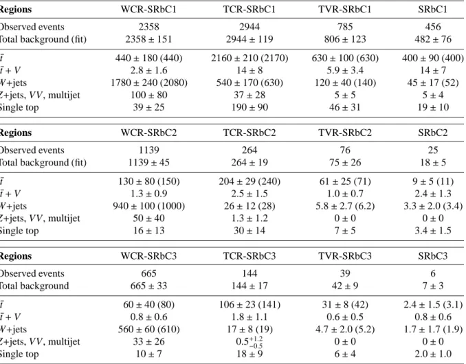
Table 2: Numbers of observed events in signal regions SRbC1–3 and the associated validation and control regions together with the estimated background predictions from the control regions only fit, for the combined electron and muon channels. Uncertainties quoted include statistical and systematic effects.

The central values of the fitted sum of backgrounds in the control regions agree with the observations by construction. The uncertainty on the total background estimate can be smaller than some of the individual uncertainties due to anticorrelations. The predicted numbers of t¯t and W +jets events using nominal cross-sections as described in Section 2 are given in parentheses.

12

Regions WCR-SRtN2 TCR-SRtN2 TVR-SRtN2 SRtN2

Observed events 165 204 23 14

Total background (fit) 165 ± 15 204 ± 16 29 ± 10 13 ± 3

t¯t 31 ± 18 (30) 139 ± 26 (138) 22 ± 8 (22) 7.5 ± 2.9 (7.5)

t¯t + V 0.4 ± 0.3 1.4 ± 0.8 0.4 ± 0.3 2.2 ± 1.2

W +jets 122 ± 28 (157) 44 ± 19 (57) 4.6 ± 2.6 (5.9) 1.5 ± 0.8 (1.9)

Z+jets, VV, multijet 11 ± 9 5 ± 4 0.1

0.4 ± 0.3

Single top 1.3

14 ± 10 2.1 ± 1.9 1.1 ± 0.5

Regions WCR-SRtN3 TCR-SRtN3 TVR-SRtN3 SRtN3

Observed events 149 175 22 7

Total background (fit) 149 ± 25 175 ± 19 28 ± 14 5 ± 2

t¯t 20 ± 15 (24) 96 ± 33 (118) 19 ± 12 (24) 1.8 ± 1.0 (2.2)

t¯t + V 0.3 ± 0.3 1.5 ± 0.9 0.48 ± 0.35 1.0 ± 0.7

W +jets 117 ± 29 (131) 55 ± 25 (61) 5.3 ± 2.6 (5.9) 1.5 ± 1.3 (1.6)

Z+jets, VV, multijet 10 ± 8 3.8 ± 3.5 0.1

0.14

Single top 1.6

19 ± 11 2.6 ± 1.9 0.53 ± 0.24

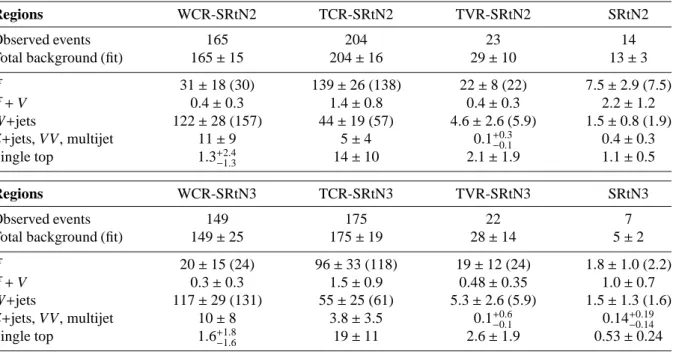
Table 3: Numbers of observed events in signal regions SRtN2 and SRtN3 and the associated validation

and control regions together with the estimated background predictions from the control regions only fit,

for the combined electron and muon channels. See further description in Table 2.

= 0b-jet ≥ 1b-jet

100 < E

< 125 GeV 60 < m

< 90 GeV 60 < m

< 90 GeV 90 < m

< 120 GeV 120 < m

< 140 GeV m

> 140 GeV

Observed events 1289 3122 1521 268 253

Total background (fit) 1289 ± 85 3122 ± 116 1535 ± 260 291 ± 61 250 ± 57

t¯t 480 ± 140 (430) 2720 ± 170 (2410) 1350 ± 249 (1200) 260 ± 60 (230) 230 ± 50 (200)

t¯t + V 2.0 ± 1.0 9 ± 4 5.6 ± 2.8 1.9 ± 0.9 2.8 ± 1.3

W+jets 730 ± 170 (880) 230 ± 120 (270) 110 ± 50 (130) 22 ± 11 (26) 12 ± 10 (14) Z+jets, VV, multijet 39 ± 35 35 ± 35 7 ± 6 1.4

0.6

Single top 31 ± 18 130 ± 70 60 ± 40 8 ± 6 6 ± 4

125 < E

< 150 GeV 60 < m

< 90 GeV 60 < m

< 90 GeV 90 < m

< 120 GeV 120 < m

< 140 GeV m

> 140 GeV

Observed events 825 1962 721 119 165

Total background (fit) 825 ± 56 1962 ± 60 755 ± 119 145 ± 23 174 ± 28

t¯t 330 ± 120 (290) 1740 ± 100 (1510) 670 ± 110 (590) 135 ± 21 (118) 162 ± 27 (141)

t¯t + V 1.4 ± 0.9 7.0 ± 3.5 3.9 ± 2.2 1.3 ± 0.7 2.9 ± 1.3

W+jets 450 ± 130 (640) 130 ± 60 (180) 47 ± 25 (68) 5 ± 5 (7) 3

−3

(5) Z+jets, VV, multijet 30 ± 24 16

−16

3.4 ± 3.4 0.4 ± 0.4 0.8

Single top 19 ± 12 78 ± 35 27 ± 19 3.4

5.7 ± 1.9

E

> 150 GeV 60 < m

< 90 GeV 60 < m

< 90 GeV 90 < m

< 120 GeV 120 < m

< 140 GeV m

> 140 GeV

Observed events 1441 2591 663 113 235

Total background (fit) 1441 ± 103 2591 ± 104 695 ± 151 101 ± 26 262 ± 34

t¯t 430 ± 180 (420) 2100 ± 180 (2030) 590 ± 120 (570) 88 ± 23 (85) 220 ± 40 (210)

t¯t + V 2.7 ± 1.7 14 ± 8 5.7 ± 3.5 2.2 ± 1.2 10 ± 5

W+jets 920 ± 210 (1110) 310 ± 120 (380) 59 ± 28 (72) 6.0 ± 3.5 (7.3) 24 ± 14 (29)

Z+jets, VV, multijet 60 ± 60 24 ± 22 2

0.4

2.1 ± 1.8

Single top 27 ± 20 140 ± 80 37 ± 26 4 ± 4 7 ± 5

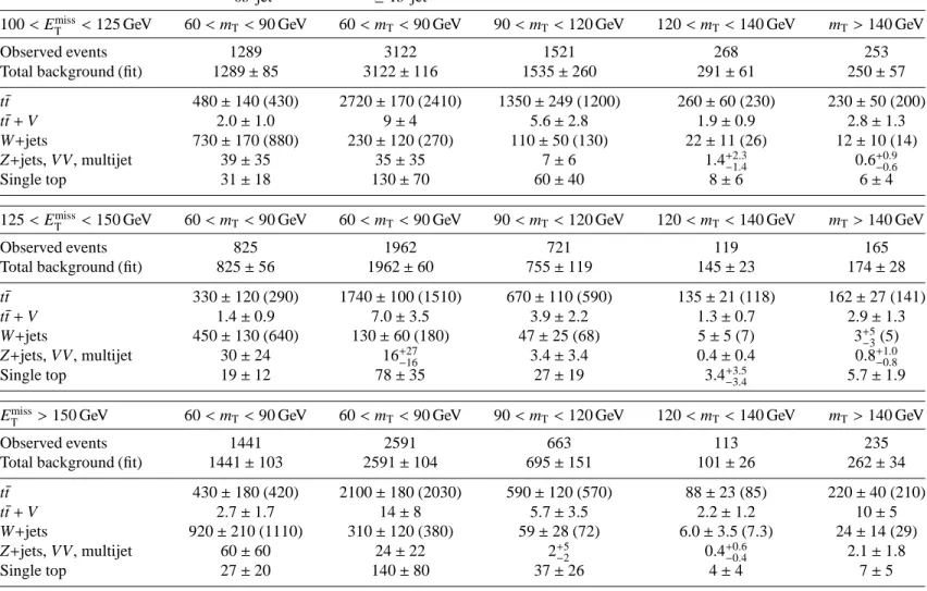
Table 4: Numbers of observed events in the SRtN1 shape matrix together with the estimated background predictions from the control regions (six bins in first two columns) only fit, for the combined electron and muon channels. See further description in Table 2.

1 4

SRtN1 SRtN2 SRtN3 SRbC1 SRbC2 SRbC3

m(˜t , LSP) = 225, 25 1075 ± 26 2.2 ± 1.0 0.9 ± 0.6 - - -

m(˜t , LSP) = 350, 150 201 ± 5 2.0 ± 0.5 0.5 ± 0.3 - - -

m(˜t , LSP) = 500, 200 71.9 ± 1.4 14.9 ± 0.6 6.8 ± 0.4 - - - m(˜t , LSP) = 600, 50 30.2 ± 0.5 13.9 ± 0.4 11.6 ± 0.3 - - - m(˜t , χ ^± ₁ , χ ⁰ ₁ ) = 200, 150, 75 - - - 233 ± 18 8 ± 4 3.1 ± 3.1 m(˜t , χ ^± ₁ , χ ⁰ ₁ ) = 350, 200, 100 - - - 166 ± 5 38.3 ± 2.5 11.1 ± 1.4 m(˜t , χ ^± ₁ , χ ⁰ ₁ ) = 600, 300, 150 - - - 26.3 ± 0.6 12.5 ± 0.4 9.0 ± 0.4 Table 5: Expected numbers of events for selected signal benchmark models in the various signal regions.

For SRtN1 shape, the sum over all E _T ^miss and m _T bins with the b-jet requirement is shown. The shown uncertainties are due to the MC sample size.

SRtN2 SRtN3 SRbC1 SRbC2 SRbC3

p ₀ -values 0.40 0.25 0.50 0.19 0.50

Table 6: Probabilities, represented by the p ₀ values, that the observed numbers of events in the various signal regions are compatible with the background-only hypothesis. p 0 values are capped at 0.5 whenever N obs < N exp .

p ₀ -values SRtN1 shape SRtN1 shape SRtN1 shape

100 < E ^miss _T < 125 GeV 125 < E _T ^miss < 150 GeV E ^miss _T > 150 GeV

120 GeV < m _T < 140 GeV 0.50 0.50 0.17

140 GeV < m _T 0.48 0.50 0.50

Table 7: Probabilities, represented by the p 0 values, that the observed numbers of events in the various signal regions are compatible with the background-only hypothesis. p 0 values are capped at 0.5 whenever N _obs < N _exp .

One-sided exclusion limits for stop signal scenarios are derived using the CL _s prescription [102], based on a simultaneous fit of the signal and control regions, where the predicted signal contamination in the control regions is taken into account. To obtain the expected combined exclusion limit, a mapping in the (m _˜t

1

, m _{χ ˜}

1

) plane is constructed by selecting the signal region with the lowest expected CL _s value for each signal grid point. For the ˜t ₁ → t + χ ˜ ⁰ ₁ decay scenario, the region of excluded stop and LSP masses at 95% CL is shown in Fig. 6. Stop masses are excluded between 200 GeV and 610 GeV for massless LSPs, and stop masses around 500 GeV are excluded for LSP masses up to 250 GeV. These limits are derived from the − 1 σ ^SUSY _theory observed limit contours (lower dotted lines). The signal region SRtN1 shape features the best expected sensitivity for the search at the lowest stop masses and also towards the region of m _˜t

1

& m _t + m _{χ ˜}

1

, SRtN2 provides the best expected sensitivity up to stop masses of about 550 GeV, and SRtN3 takes over for higher stop masses. For the ˜t ₁ → b + χ ˜ ^± ₁ decay the exclusion limits are shown in Fig. 7 for m _{χ ˜}

1

= 150 GeV and Fig. 8 for m _{χ ˜}

1

= 2 × m _{χ ˜}

1

. Stop masses are excluded up to 410 GeV for

massless LSPs and m χ _˜

= 150 GeV. The results of this search significantly extend previous stop mass

Events

1 10 102

103

104

105

106

107

Data 2012 Standard Model (SM)

t t W+Jets

+V, single top, multijets t

t Z+Jets, VV = 150 [GeV]

χ0

= 350, m

~t m

L dt = 20.7 fb-1

∫

= 8 TeV, s

channel µ e+

Preliminary ATLAS

tN1 shape:

< 125 GeV

miss

100 GeV < ET

[GeV]

m

W-CR 60-90 90-120 120-140 >140

Data/SM

0.5 1 1.5

Events

1 10 102

103

104

105

106

107 ^{Data 2012}

Standard Model (SM) t

t W+Jets

+V, single top, multijets t

t Z+Jets, VV = 150 [GeV]

χ0

= 350, m

~t m

L dt = 20.7 fb-1

∫

= 8 TeV, s

channel µ e+

Preliminary ATLAS

tN1 shape:

< 150 GeV

miss

125 GeV < ET

[GeV]

m

W-CR 60-90 90-120 120-140 >140

Data/SM

0.5 1 1.5

Events

1 10 102

103

104

105

106

107 ^{Data 2012}

Standard Model (SM) t

t W+Jets

+V, single top, multijets t

t Z+Jets, VV = 150 [GeV]

χ0

= 350, m

~t m

L dt = 20.7 fb-1

∫

= 8 TeV, s

channel µ e+

Preliminary ATLAS

tN1 shape:

> 150 GeV

miss

ET

[GeV]

m

W-CR 60-90 90-120 120-140 >140

Data/SM

0.5 1 1.5

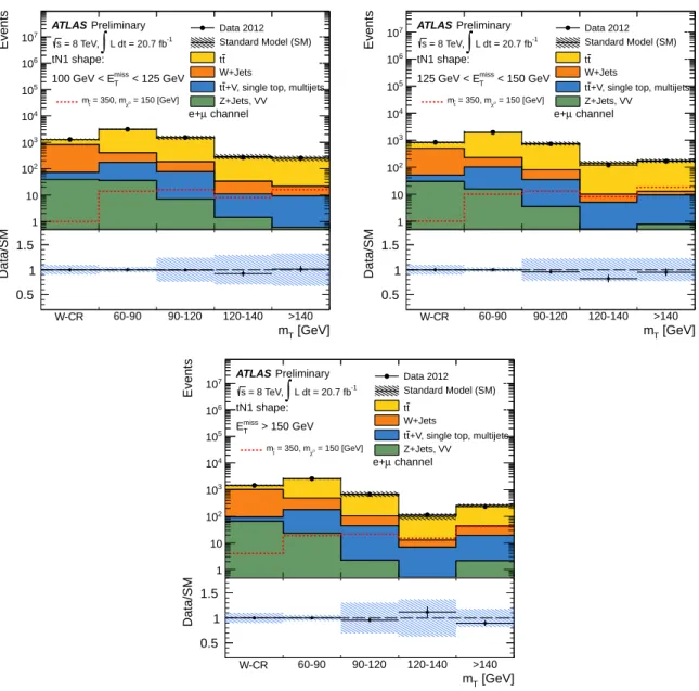
Figure 5: Background fit results for the SRtN1 shape fit. In this fit, the t¯t and W +jets backgrounds are normalized in the W +jets control region (WCR) and the t¯t control region (indicated by 60-90 in this figure) for each of the three E ^miss _T slices simultaneously. The uncertainties (statistical and systematic) estimated in the control regions are fully extrapolated to the m _T > 90 GeV bins and displayed as a shaded area on the sum of the backgrounds. One selected signal model is shown for comparison. The fit shown in this plot is only for illustration purposes, since the fit used for the limits uses all 15 signal and control bins simultaneously, which allows to constrain the uncertainties in the signal bins.

16

[GeV]

t

m ~

200 300 400 500 600 700 800

[ G e V]

0✁

m

0 50 100 150 200 250 300 350 400

t

<

m

1 0

✂

✄

- m

t1

m

1 0

☎

t

1✝

~ t production, t

~ t

~

exp

) 1 Expected limit ( !

Expected limit (HCP12)

theory

) 1

Observed limit ( ! ATLAS Preliminary

All limits at 95% CL

T

1-lepton + jets + E

=8 TeV s

-1

, L dt = 20.7 fb

Figure 6: Expected (black dashed) and observed (red solid) 95% CL excluded region (under the curve) in the plane of m _{χ ˜}

1

vs. m ˜t

, assuming B (˜t 1 → t ˜ χ ⁰ ₁ ) = 100%. All uncertainties except the theoretical signal cross-section uncertainties are included. The contours of the yellow band around the expected limit are the ± 1 σ results. The dotted red lines around the observed limit illustrate the change in the observed limit as the nominal signal cross-section is scaled up and down by the theoretical uncertainty. For comparison the light grey dashed line shows the expected exclusion limit of the ATLAS stop 1-lepton search on 13 fb ^{− 1} [24].

limits, especially for the ˜t ₁ → b + χ ˜ ^± ₁ decay scenario and for the ˜t ₁ → t + χ ˜ ⁰ ₁ decay scenario near the m _˜t

1

& m t + m _{χ ˜}

1

diagonal.

Figure 9 compares the upper cross section limits at 95% CL for a fixed LSP mass of 50 GeV — which covers a large range of possible top squark masses and also covers quite nicely all three SRtN signal regions — obtained for signal models where ˜t ₁ is purely ˜t _L or mostly ( ∼ 70%) ˜t _R . The mostly-˜t _R mixing composition is used for all other scenarios studied in this note. The weaker ˜t _L model exclusion is mainly the result of a reduced lepton and m _T acceptance. The acceptance is affected because the polarization of the top quark changes as a function of the field content of the supersymmetric particles, changing the boost of the lepton in the top quark decay. The excluded ˜t ₁ mass reach of the ˜t _L model is reduced by about 75 GeV, for the assumed LSP mass.

Generic limits on beyond-SM contributions are derived from the same simultaneous fit as used for

calculating the CL _s values but without signal model-dependent inputs — the generic signal model in-

cludes neither signal contamination in the control regions, nor experimental and theoretical signal sys-

tematic uncertainties. In the case of the shape fit, the generic signal model assumes, for each E _T ^miss slice,

the presence of events only in the tightest m _T bin, the signal being absent in the other bins. The resulting

[GeV]

t

m ~

200 250 300 350 400 450 500 550 600

[ G e V]

m

0 50 100 150 200 250

= 150 GeV

! 1

✁

1 , m + 0

W (*) 1

, ! 1

b+ !

t 1

production, ~ t 1

~ t 1

~

exp ) 1 Expected limit ( !

Expected limit (HCP12)

theory ) 1 SUSY

Observed limit ( !

ATLAS Preliminary

All limits at 95% CL

T

1-lepton + jets + E miss

=8 TeV s

-1 , L dt = 20.7 fb

( = 150 GeV)

! 1

✂

> m

1 0

✂

m

Figure 7: Expected (black dashed) and observed (red solid) 95% CL excluded region (under the curve) in the plane of m _{χ ˜}

1

vs. m _˜t

, assuming B (˜t ₁ → b ˜ χ ^± ₁ ) = 100%, B ( ˜ χ ^± ₁ → W ^∗ χ ˜ ⁰ ₁ ) = 100%, and m χ _˜

1

= 150 GeV.

All uncertainties except the theoretical signal cross-section uncertainties are included. The contours of the yellow band around the expected limit are the ± 1 σ results. The dotted red lines around the observed limit illustrate the change in the observed limit as the nominal signal cross-section is scaled up and down by the theoretical uncertainty. For comparison the light grey dashed line shows the expected exclusion limit of the ATLAS stop 1-lepton search on 13 fb ^{− 1} [24].

18

[GeV]

t ~ 1

m

100 200 300 400 500 600 700

[ G e V] 1 0 m

60 80 100 120 140 160 180 200 220 240

260

0

m

= 2 !

"

1

✁

1 , m + 0

W (*) 1

"

1 ,

"

1 b+

~ t production, t 1

~ t 1

~

ATLAS Preliminary

T

1-lepton + jets + E miss

=8 TeV s

-1 , L dt = 20.7 fb

)

1 0

✂

✄

! m

= 2

1

"

✂

✄

( m

1

"

✂

✄

+m

<

m

t1

m

exp ) 1

"

Expected limit (

Expected limit (HCP12)

theory ) 1 SUSY

"

Observed limit (

1-2 leptons (2011)

All limits at 95% CL

Figure 8: Expected (black dashed) and observed (red solid) 95% CL excluded region (inside the curve) in the plane of m _{χ ˜}

1

vs. m _˜t

, assuming B (˜t ₁ → b ˜ χ ^± ₁ ) = 100%, B ( ˜ χ ^± ₁ → W ^∗ χ ˜ ⁰ ₁ ) = 100%, and m _{χ ˜}

1

= 2 × m _{χ ˜}

. All uncertainties except the theoretical signal cross-section uncertainties are included. The contours of the yellow band around the expected limit are the ± 1 σ results. The dotted red lines around the observed limit illustrate the change in the observed limit as the nominal signal cross-section is scaled up and down by the theoretical uncertainty. For comparison the blue filled area shows the observed 2011 ATLAS

˜t ₁ → b + χ ˜ ^± ₁ exclusion limit [28], making the same signal assumption (m χ _˜

= 2 × m _{χ ˜}

1

). The dashed and dotted dark blue lines show the corresponding expected and observed − 1 σ ^SUSY _theory limits, respectively.

Also for for comparison, the light grey dashed line shows the expected exclusion limit of the ATLAS

stop 1-lepton search on 13 fb ^{− 1} [24].