Search for direct stop production in events with missing transverse momentum and two b-jets using 12.8 fb

ATLAS-CONF-2013-001 07/01/2013

ATLAS NOTE

ATLAS-CONF-2013-001

21 December 2012 Minor revision: 5 January 2013

Search for direct stop production in events with missing transverse momentum and two b-jets using 12.8 fb

of pp collisions at

√ s = 8 TeV with the ATLAS detector

The ATLAS Collaboration

Abstract

The results of the search for direct pair production of bottom squarks are reinter- preted in terms of direct pair production of top squarks decaying exclusively into a bottom quark and a chargino. The dataset used corresponds to an integrated lumi- nosity of 12.8

of

collisions at

s=8

TeV recorded by the ATLAS detector at the LHC. Assuming that the mass difference between the chargino and the lightest neutralino is small (

GeV), top squarks with masses

GeV are excluded at 95% confidence level for

GeV and neutralino masses up to 300 GeV are excluded for

GeV. In the case of larger mass differences (

GeV) the top squark and neutralino mass limits weaken by up to 100 GeV.

Note number revised on 5 January 2013

c Copyright 2013 CERN for the benefit of the ATLAS Collaboration.

Reproduction of this article or parts of it is allowed as specified in the CC-BY-3.0 license.

1 Introduction

Supersymmetry (SUSY) [1–9] provides a solution to the hierarchy problem of the Standard Model (SM) by introducing supersymmetric partners of the known bosons and fermions [10–

13]. In

-parity conserving SUSY scenarios SUSY particles are produced in pairs at the LHC.

Each SUSY particle subsequently decays (possibly via intermediate SUSY particles) to Standard Model particles and a lightest supersymmetric particle (LSP), which is stable. This generically results in collider signatures with relatively large missing transverse momentum.

Naturalness arguments [14–16] require the masses of the superpartners closely connected to the Higgs sector to be near the electroweak scale. In particular, the lightest of the third genera- tion squarks (the stop and sbottom), the fermionic partners of the Higgs bosons (the higgsinos), and to a lesser extent, the partner of the gluon (the gluino) are required to be relatively light.

The other SUSY particles, on the other hand, are not constrained by naturalness criteria, and may have masses much larger than 1 TeV.

A search for pair production of the lightest sbottom particle (

), each decaying into a bot- tom quark (b) and a neutralino (

) has been recently performed in ATLAS [17]. Pair produced stops (

) may mimic this signature if they decay into a

-quark and a chargino (

), and the mass difference between the chargino and the neutralino is small. This possibility is a general feature of scenarios where the LSP is mainly higgsino or wino, and the other gauginos are much heavier.

In this note, the search for the pair production of bottom squarks presented in Ref. [17] is reinterpreted in terms of stop pair production. A simplified scenario is considered, in which the stop decays exclusively via

, and

decays via

, with

and

representing different fermion types according to the SM branching ratios of the

boson.

In case of small values for

,

and

are soft and may have transverse mo- menta below the reconstruction thresholds applied in the analysis. This leads to the final state signature of two

for which the sbottom pair production was designed.

Two different values of

are considered: 5 GeV and 20 GeV. In addition, a few models with

∆m=10

GeV are considered to evaluate the analysis efficiency in an intermediate scenario. In this study, only models that are not excluded by the LEP lower limit on the chargino mass of 103.5 GeV [18] are considered.

In Section 2, differences in selection efficiency between top squark pair events and bottom squark pair events are discussed. The results are presented in Section 3, and conclusions are given in Section 4.

2 Comparison with the search for sbottom pair events

Since differences between stop and sbottom production cross sections are negligible [19], the

main difference between the analysis sensitivities is the eventual change in acceptances. A

summary of the different signal regions considered in the analysis of Ref. [17] can be found

in Table 1. The sensitivity of this analysis (optimised for sbottom pair production) to stop

pair production depends strongly on

. For a small mass splitting, the signal acceptance

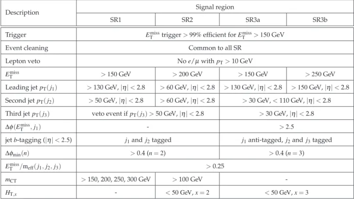
Description Signal region

SR1 SR2 SR3a SR3b

Trigger ET^misstrigger>99%efficient forET^miss>150GeV

Event cleaning Common to all SR

Lepton veto Noe/µwithpT>10 GeV

E_T^miss >150GeV >200GeV >150GeV >250GeV

Leading jetpT(j1) >130 GeV,|η|<2.8 >60 GeV,|η|<2.8 >130GeV,|η|<2.8 >150GeV,|η|<2.8 Second jetpT(j2) >50 GeV,|η|<2.8 >60 GeV,|η|<2.8 >30 GeV,<110 GeV,|η|<2.8 Third jetpT(j3) veto event ifpT(j3)>50 GeV,|η|<2.8 >30 GeV,|η|<2.8

∆φ(ET^miss,j1) - >2.5

jetb-tagging (|η|<2.5) j1andj2tagged j1anti-tagged, j2andj3tagged

∆φmin(n) >0.4 (n=2) >0.4 (n=3)

ET^miss/m_eff(j1,j2,j3) >0.25

mCT >150, 200, 250, 300 GeV >100 GeV -

HT,x - <50 GeV,x=2 <50 GeV,x=3

Table 1: Summary of the event selection in each signal region. The leading, subleading and 3rd leading jet are referred to as

,

and

, respectively.

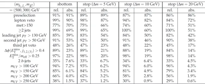
Table 2 compares the SR1 selection efficiencies for sbottom pair production and stop pair production models with

1,t˜1=500

GeV,

GeV, and

GeV, 10 GeV and 20 GeV.

For stop pair production, the fraction of events passing the lepton veto decreases with increas- ing

remaining selection steps, including the veto on the third jet, have similar efficiencies for all the samples considered.

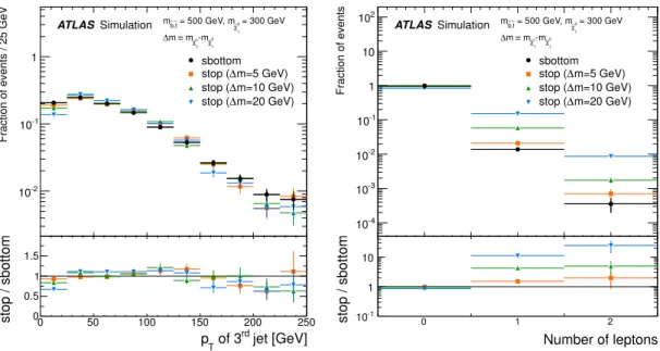
The distributions of the third hardest jet and the number of leptons are shown in Figure 1, comparing the models considered in Table 2. Figure 2 shows the distributions of the

vari- ables used in SR2 and SR3, for models with

1,t˜1 =600

GeV,

GeV and

1,˜t1 =500

GeV,

GeV. The efficiencies of selections on the

variables used in SR2 and SR3 agree within a few percent for the sbottom and the corresponding stop pair sample with

∆m=5

GeV. With larger

with

GeV,

GeV and

GeV, the

GeV selection criterion is found to reduce the stop signal event yield by a factor of two compared to the corresponding sbottom scenario.

3 Results and interpretation

The results are interpreted in stop pair production scenarios in which the stop is assumed to

decay via

with a 100% branching ratio. The mass difference between

and

is

taken to be either 5 or 20 GeV. The signal samples are generated using

[20] interfaced

to Pythia 6 [21], using the PDF set

[22].

(m˜b₁,t˜₁,mχ˜1⁰) sbottom stop (∆m=5GeV) stop (∆m=10GeV) stop (∆m=20GeV)

= (500,300)GeV rel. abs. rel. abs. rel. abs. rel. abs.

preselection 91% 91% 89% 89% 87% 87% 86% 86%

lepton veto 99% 90% 98% 87% 94% 82% 84% 72%

met>150 77% 70% 75% 66% 74% 60% 71% 51%

≥2 jets 99% 69% 99% 65% 100% 60% 100% 51%

leading jetp_T>130GeV 85% 59% 83% 54% 84% 50% 82% 42%

second jetpT>50GeV 91% 53% 92% 50% 91% 46% 90% 38%

third jet veto 48% 26% 47% 23% 48% 22% 45% 17%

∆φ(E_T^miss,j1,2,(3))>0.4 89% 23% 89% 21% 88% 19% 84% 14%

ET^miss/meff>0.25 97% 22% 98% 20% 98% 19% 98% 14%

2b-jets 35% 7.6% 33% 6.7% 34% 6.4% 33% 4.5%

mCT>100GeV 94% 7.2% 93% 6.2% 94% 6.0% 96% 4.3%

m_CT>150GeV 85% 6.1% 84% 5.2% 81% 4.9% 79% 3.4%

mCT>200GeV 66% 4.0% 62% 3.2% 58% 2.8% 56% 1.9%

m_CT>250GeV 38% 1.5% 37% 1.2% 30% 0.9% 29% 0.6%

Table 2: Selection efficiencies for a sbottom signal point with

1=500

GeV and

GeV (second and third columns), and three stop signal points with

GeV,

GeV for

∆m=5

GeV, 10 GeV and 20 GeV. The absolute selection efficiencies are computed with respect to the total number of simulated events, whereas relative efficiencies are computed with respect to the previous selection criterion. All numbers are extracted from samples whose total size is roughly 10000 events.

Experimental and theoretical uncertainties on the signal are included using the prescrip- tions discussed in Ref. [17].

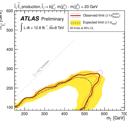
The 95% confidence level (C.L.) exclusion limits obtained using the

prescription [23] are shown in Fig. 3 for

GeV and in Fig. 4 for

GeV. The signal region with the best expected

exclusion limit is used to derive the limit for each signal point.

If

GeV, stop quark masses up to 580 GeV are excluded at 95% C.L. for

GeV and 480 GeV for

GeV. Assuming

(∆m

) GeV, neutralino masses up to 300 (250) GeV are excluded for

GeV.

4 Conclusions

The results of Ref. [17], based on 12.8 fb

of

s=8

TeV

collision data recorded by the ATLAS detector, are interpreted in scenarios where pair produced stops decay into a chargino and a bottom quark.

For

GeV, stop masses up to 580 GeV are excluded at 95% C.L. for

GeV and

480 GeV for

GeV. Assuming

GeV, neutralino masses up to 300 GeV are excluded

for

GeV. Assuming

GeV, neutralino masses up to 250 GeV are excluded for

GeV.

0 50 100 150 200 250

Fraction of events / 25 GeV

10-2

10-1

1 sbottom

m=5 GeV)

∆ stop (

m=10 GeV)

∆ stop (

m=20 GeV)

∆ stop (

= 300 GeV

0 1

= 500 GeV, mχ∼

~t ,

~b

m

0 1

-mχ∼

± 1

mχ∼

m ≡

∆ ATLAS Simulation

jet [GeV]

of 3rd

pT

0 50 100 150 200 250

stop / sbottom ⁰

0.5 1

1.5 0 0.5 1 1.5 2 2.5 3

Fraction of events

10-4

10-3

10-2

10-1

1 10 102

sbottom m=5 GeV)

∆ stop (

m=10 GeV)

∆ stop (

m=20 GeV)

∆ stop (

= 300 GeV

0 1

= 500 GeV, mχ∼

~t , b~

m

0 1

-mχ∼

± 1

mχ∼

m ≡

∆ ATLASSimulation

Number of leptons

0 1 2

stop / sbottom ^-110

1 10

Figure 1: Comparison of distributions (normalised to unit area) for a sbottom signal point with

1 =500

GeV and

GeV, and three stop signal points with

GeV,

GeV and

GeV, 10 GeV and 20 GeV. The

of the third highest momentum jet (left)

and the number of electrons and muons with

GeV (right). The distribution of the

of the third highest momentum jet is produced after requiring all selection criteria up to

and including the

GeV requirement on the second jet in Table 2. The distribution of

the number of leptons is produced after the preselection. Only statistical uncertainties arising

from the limited size of simulated samples are shown. The bottom panel in each plot shows

the ratios of the histogram entries from the stop pair samples and the sbottom pair sample. The

final bin in the histograms includes the overflow.

0 50 100 150 200 250 300

Fraction of events / 30 GeV

10-3

10-2

10-1

1 sbottom

m=5 GeV)

∆ stop (

m=20 GeV)

∆ stop (

= 100 GeV

0 1

= 600 GeV, mχ∼

~t ,

~b

m

0 1

-mχ∼

± 1

mχ∼

≡

∆m ATLAS Simulation

[GeV]

HT,2

0 50 100 150 200 250 300

stop / sbottom

1 2 3

0 50 100 150 200 250 300

Fraction of events / 30 GeV

10-2

10-1

1 10

sbottom m=5 GeV)

∆ stop (

m=20 GeV)

∆ stop (

= 450 GeV

0 1

= 500 GeV, mχ∼

~t , b~

m

0 1

-mχ∼

± 1

mχ∼

≡

∆m ATLASSimulation

[GeV]

HT,3

0 50 100 150 200 250 300

stop / sbottom ⁰

0.5 1 1.5

Figure 2: Comparison of distributions normalised to unit area for a sbottom pair signal point and two stop pair signal points with

and 20 GeV. Left:

distribution for

1 =m_t^˜1 = 600

GeV and

GeV. Right:

distribution for

1=m_t^˜1=500

GeV and

GeV.

The distribution of

is produced after requiring all selection criteria up to and including the

GeV requirement on the second jet in Table 2. The distribution of

is produced after requiring the leading jet to have

GeV and two additional jets with

GeV.

Only statistical uncertainties arising from the limited size of simulated samples are shown. The

bottom panel in each plot shows the ratios of the histogram entries from the stop pair samples

to the sbottom pair sample. The final bin in the histograms includes the overflow.

[GeV]

t1

m~

200 300 400 500 600 700

[GeV]0 1χ∼m

100 150 200 250 300 350 400 450 500 550 600

forbidden

1

±χ b∼

→₁

~t

) = 5 GeV

1

χ∼0

) - m(

1

χ∼± 1, m(

χ∼±

→ b t1

production, ~ t1

~

1-

~t

ATLAS

=8 TeV s

-1, L dt = 12.8 fb

∫

theory) σSUSY

±1 Observed limit (

exp) σ

±1 Expected limit ( All limits at 95% CL

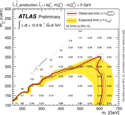
Figure 3: Expected and observed 95% C.L. exclusion limits in the

plane for

GeV. The black, dashed line shows the expected limit if theoretical uncertainties on the signal

are neglected. The yellow band shows the

uncertainty on the expected limit. The red solid

line shows the nominal observed limit, while the red dashed lines show its variation if theory

uncertainties on the signal are taken into account.

[GeV]

t1

m~

200 300 400 500 600 700

[GeV]0 1χ∼m

100 200 300 400 500 600

forbidden

1

±χ

∼

→₁ b

~t

) = 20 GeV

1

χ∼0

) - m(

1

χ∼± 1, m(

χ∼±

→ b t1

production, ~ t1

~

1-

~t

ATLAS

=8 TeV s

-1, L dt = 12.8 fb

∫

theory) σSUSY

±1 Observed limit (

exp) σ

±1 Expected limit ( All limits at 95% CL

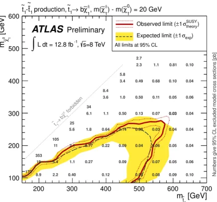
Figure 4: Expected and observed 95% C.L. exclusion limits in the

plane for

GeV. The black, dashed line shows the expected limit if theoretical uncertainties on the signal

are neglected. The yellow band shows the

uncertainty on the expected limit. The red solid

line shows the nominal observed limit, while the red dashed lines show its variation if theory

uncertainties on the signal are taken into account.

A Auxiliary material

[GeV]

b1

or m~ t1

m~

200 300 400 500 600 700

[GeV]0 1χ∼m

100 200 300 400 500 600

) + 5 GeV < 103.5 GeV

1

χ∼0

m(

forbidden

1 0χ b∼

→₁

~b or

1

±χ b∼

→1

~t

production b1

-~ b1

or ~ t1

-~ t1

~

ATLAS

=8 TeV s

-1, L dt = 12.8 fb

∫

expected observed expected observed expected observed

1

χ∼±

→ b t1

production, ~ t1

-~ t1

~

) = 5 GeV

0

χ∼1

±, χ∼1

∆m(

1

χ∼±

→ b t1

production, ~ t1

-~ t1

~

) = 20 GeV

0

χ∼1

±, χ∼1

∆m(

1

χ∼0

→ b b1

production, ~ b1

-~ b1

~

ATLAS-CONF-2012-165

not included

theory

σSUSY

All limits at 95% CL,

Figure 5: Expected and observed 95% C.L. exclusion limits on sbottom pair production in the

plane, together with the expected and observed 95% C.L. exclusion limits for stop

pair production in the

plane for

GeV and 20 GeV. The theory uncertainty on

the signal is not shown.

[GeV]

t1

m~

200 300 400 500 600 700

[GeV]0 1χ∼m

100 150 200 250 300 350 400 450 500 550 600

Numbers give 95% CL excluded model cross sections [pb]

forbidden

1

±χ

∼

→₁ b

~t

0.03

0.02

0.03

0.18 0.03

3.1

0.64

16

0.03

0.02 0.02 132

0.25 37

0.23

0.32

2.8

0.92

6.1

0.03

0.06

0.08 0.26

0.09 1.1

0.91

0.02 0.43

0.09

0.02

0.02 0.52

0.25

0.03

12

0.02 0.58

0.42 98

3.5

0.03

0.02 0.08 0.55

0.71

0.02

0.14 50

1.7

0.03 261

3.0

4.6

1.5

0.19

0.02 3.9

0.06

0.03 0.07

0.02 0.04 0.04

) = 5 GeV

1

χ∼0

) - m(

1

χ∼± 1, m(

χ∼±

→ b t1

production, ~ t1

~

1-

~t

ATLAS

=8 TeV s

-1, L dt = 12.8 fb

∫

theory) σSUSY

±1 Observed limit (

exp) σ

±1 Expected limit ( All limits at 95% CL

Figure 6: Expected and observed 95% C.L. exclusion limits in the

plane for

GeV. The black, dashed line shows the expected limit if theory uncertainties on the signal are

neglected. The yellow band shows the

uncertainty on the expected limit. The red solid

line shows the nominal observed limit, while the red dashed lines show its variation if theory

uncertainties on the signal are taken into account. The overlaid numbers give the observed

upper limit on the signal cross section, in pb. For clarity, numbers of the first row (column)

have been shifted upwards (right) by 10 GeV.

[GeV]

t1

m~

200 300 400 500 600 700

[GeV]0 1χ∼m

100 200 300 400 500 600

Numbers give 95% CL excluded model cross sections [pb]

forbidden

1

±χ

∼

→ b t1

~

0.07

0.09 0.07

0.09

0.40 0.08

5.4

2.2

0.04

0.05 0.04 0.64

0.50

0.09 0.77

3.4

19

0.10

0.13 0.68

0.12 2.1

3.6

0.04 25

1.1

0.22

0.04

0.05 0.49

0.81

0.06 34

0.06 1.0

1.1

0.03

11

0.08

0.09 353

0.14 1.1

1.8

0.05

0.27

5.8

8.4

6.1

0.10 105

5.6

8.9

2.7 2.3

0.50

0.04

0.10

172

0.06 0.11

0.04 0.03 0.03

) = 20 GeV

1

χ∼0

) - m(

1

χ∼± 1, m(

χ∼±

→ b t1

production, ~ t1

~

1-

~t

ATLAS

=8 TeV s

-1, L dt = 12.8 fb

∫

theory) σSUSY

±1 Observed limit (

exp) σ

±1 Expected limit ( All limits at 95% CL

Figure 7: Expected and observed 95% C.L. exclusion limits in the

plane for

GeV. The black, dashed line shows the expected limit if theory uncertainties on the signal are

neglected. The yellow band shows the

uncertainty on the expected limit. The red solid

line shows the nominal observed limit, while the red dashed lines show its variation if theory

uncertainties on the signal are taken into account. The overlaid numbers give the observed

upper limit on the signal cross section, in pb. For clarity, the first column number has been

shifted right by 10 GeV.

References

[1] H. Miyazawa, Baryon Number Changing Currents, Prog. Theor. Phys.

(1966) 1266–1276.

[2] P. Ramond, Dual Theory for Free Fermions, Phys. Rev.

(1971) 2415–2418.

[3] Y. A. Gol’fand and E. P. Likhtman, Extension of the Algebra of Poincare Group Generators and Violation of p Invariance, JETP Lett.

(1971) 323–326. [Pisma

Zh.Eksp.Teor.Fiz.13:452-455,1971].

[4] A. Neveu and J. H. Schwarz, Factorizable dual model of pions, Nucl. Phys.

(1971) 86–112.

[5] A. Neveu and J. H. Schwarz, Quark Model of Dual Pions, Phys. Rev.

(1971) 1109–1111.

[6] J. Gervais and B. Sakita, Field theory interpretation of supergauges in dual models, Nucl. Phys.

B34

(1971) 632–639.

[7] D. V. Volkov and V. P. Akulov, Is the Neutrino a Goldstone Particle?, Phys. Lett.

(1973) 109–110.

[8] J. Wess and B. Zumino, A Lagrangian Model Invariant Under Supergauge Transformations, Phys. Lett.

(1974) 52.

[9] J. Wess and B. Zumino, Supergauge Transformations in Four-Dimensions, Nucl. Phys.

(1974) 39–50.

[10] S. Weinberg, Implications of Dynamical Symmetry Breaking, Phys. Rev.

(1976) 974–996.

[11] E. Gildener, Gauge Symmetry Hierarchies, Phys. Rev.

(1976) 1667.

[12] S. Weinberg, Implications of Dynamical Symmetry Breaking: An Addendum, Phys. Rev.

(1979) 1277–1280.

[13] L. Susskind, Dynamics of Spontaneous Symmetry Breaking in the Weinberg- Salam Theory, Phys. Rev.

(1979) 2619–2625.

[14] R. Barbieri and G. Giudice, Upper Bounds on Supersymmetric Particle Masses, Nucl.Phys.

B306

(1988) 63.

[15] B. de Carlos and J. Casas, One loop analysis of the electroweak breaking in supersymmetric models and the fine tuning problem, Phys.Lett.

(1993) 320–328,

arXiv:hep-ph/9303291 [hep-ph]

.

[16] M. Papucci, J. T. Ruderman, and A. Weiler, Natural SUSY Endures, JHEP

(2012) 035,

.

[17] ATLAS Collaboration, Search for scalar bottom pair production in final states with missing

[19] W. Beenakker, S. Brensing, M. Kramer, A. Kulesza, E. Laenen, and I. Niessen,

Supersymmetric top and bottom squark production at hadron colliders, JHEP

(2010) 098,

.

[20] M. Bahr, S. Gieseke, M. Gigg, D. Grellscheid, K. Hamilton, et al., Herwig++ Physics and Manual, Eur. Phys. J.

(2008) 639–707,

.

[21] T. Sj ¨ostrand, S. Mrenna, and P. Skands, PYTHIA 6.4 physics and manual, JHEP

(2006) 026.

[22] J. Pumplin et al., New generation of parton distributions with uncertainties from global QCD analysis, JHEP

(2002) 012.

[23] G. Cowan, K. Cranmer, E. Gross, and O. Vitells, Asymptotic formulae for likelihood-based

tests of new physics, Eur. Phys. J.

(2011) 1–19.