A TLAS-CONF-2017-053 10 July 2017
ATLAS CONF Note
ATLAS-CONF-2017-053
5th July 2017
Search for doubly-charged Higgs boson production in multi-lepton final states with the ATLAS detector
using proton-proton collisions at √
s = 13 TeV
The ATLAS Collaboration
A search for doubly-charged Higgs bosons with pairs of prompt, isolated, highly ener- getic leptons with the same electric charge is presented. The search uses the pp data sample corresponding to 36.1 fb −1 of integrated luminosity collected in 2015 and 2016 by the ATLAS detector at the LHC at the centre-of-mass energy of 13 TeV. The search scans through various doubly-charged Higgs branching ratio (Br) hypotheses, where Br( H ±± → e ± e ± ) + Br( H ±± → e ± µ ± ) + Br (H ±± → µ ± µ ± ) ≤ 100%, in several exclusive signal regions.
No significant evidence of signal was observed and corresponding limits on the production cross-section and consequently the lower limit on m( H ±± ) were derived at 95% CL. Defining
` = e, µ, the observed lower limit on H ±± L mass varies from 770 GeV to 870 GeV (850 GeV expected) for Br (H ±± → ` ± ` ± ) = 100% and is still above 450 GeV, for both observed and expected, for Br( H ±± → ` ± ` ± ) = 10% for any combination of partial branching ratios.
c
2017 CERN for the benefit of the ATLAS Collaboration.
Reproduction of this article or parts of it is allowed as specified in the CC-BY-4.0 license.
1 Introduction
Events with two highly energetic, isolated, prompt leptons with the same electric charge (same-charge leptons) are produced very rarely in a proton-proton collision according to the predictions of the Stand- ard Model (SM), but they may occur with a higher rate in various beyond-the-Standard Model (BSM) theories. This analysis studies BSM theories that contain a doubly-charged Higgs particle using the ob- served invariant mass of same-charge lepton pairs. In the absence of evidence for a signal, lower limits on the mass of the H ±± particle are set at the 95% confidence level, assuming the theoretical production cross-section.
Doubly-charged Higgs bosons can arise in a large variety of BSM theories, namely in left-right sym- metric models [1–5] (LRSM), Higgs triplet models [6, 7], the little Higgs model [8], Type II seesaw models [9–13], the Georgi-Machacek model [14], scalar singlet dark matter [15], and the Zee-Babu neut- rino mass model [16–18]. Theoretical studies [19–21] indicate that the doubly-charged Higgs would be predominantly pair produced via the Drell-Yan process at the LHC.
Doubly-charged Higgs particles can couple to either left-handed or right-handed leptons. In the LRSM the two cases are distinguished and denoted H L ±± and H R ±± . The cross-section for H L ±± H ∓∓ L production is about 2.3 times larger than the one for H ±± R H R ∓∓ due to the different couplings to the Z boson [22]. Along with the leptonic decay, the H ±± particle can decay into a pair of W bosons as well. For low values of the Higgs triplet vacuum expectation value v ∆ it decays almost exclusively to leptons and for high values of v ∆ mostly to a pair of W bosons [9, 12]. In this analysis the coupling to W bosons is assumed to be negligible and only the pair production via the Drell-Yan process is considered. The Feynman diagram of the production mechanism is presented in Figure 1.
The analysis studies the case where the H ±± particle decays only into electrons and muons, denoted as
`, and other invisible final states that have no impact on the signal yield in the signal regions, denoted as X . The total assumed decay branching ratio of H ±± is therefore Br (H ±± → e ± e ± ) + Br (H ±± → e ± µ ± ) + Br( H ±± → µ ± µ ± ) + Br (H ±± → X ) = Br (H ±± → ` ± ` ± ) + Br (H ±± → X ) = 100%. Moreover, the decay width is assumed to be negligible compared to the detector resolution, which is compatible with theoretical predictions. Two, three, and four lepton signal regions are defined to select the majority of such events and the regions are further divided into unique flavour categories (e or µ) to increase the sensitivity. In the final interpretation of the results, the decay into invisible X states is intended to account for decays into particles not directly considered in the selection of the analysis or outside the acceptance, like τ leptons. The partial decay width of H ±± to leptons is given by:
Γ ( H ±± → ` ± ` 0± ) = k h 2 ``
08π m( H ±± ), (1)
where k = 1 if both leptons have the same flavour (` = ` 0 ) and k = 2 if they have di ff erent flavours. The factor h ``
0has an upper bound that depends on the flavour combination [23, 24] and in this analysis only prompt decays of the H ±± bosons (cτ < 10 µm) are considered, corresponding to h ``
0& 1.5 × 10 −6 for m(H ±± ) = 200 GeV. In general, there is no preference for τ decays, as there is no coupling to lepton mass unlike for the SM Higgs.
Further motivation for studying the case where Br (H ±± → ` ± ` ± ) < 100% are type-II see-saw models with specific neutrino mass hypotheses and consequently a fixed branching ratio combination [13, 25, 26]
which does not necessarily correspond to Br (H ±± → ` ± ` ± ) = 100%.
q
q
γ/Z
H ++
H −−
ℓ + ℓ + ℓ −
ℓ −
Figure 1: Feynman diagram of the pair production pp → H
±±H
∓∓process. The analysis studies only the electron and muon channels, where at least one of the lepton pairs are e
±e
±, e
±µ
±, or µ
±µ
±.
The ATLAS collaboration has already published similar studies and the most stringent constraints origin- ate from Ref. [27] using the 20.3 fb −1 of integrated luminosity taken in 2012 at a centre-of-mass energy of 8 TeV, where the lower limit on the H L ±± mass was observed to vary between 465 GeV and 550 GeV for Br (H ±± → ` ± ` ± ) = 100%, depending on the lepton flavours. The current analysis expands upon prior work by using 36.1 fb −1 of integrated luminosity collected in 2015 and 2016 at the centre-of-mass energy of 13 TeV. Similar searches were also performed by the CMS collaboration [28].
2 The ATLAS Detector
The ATLAS detector [29] at the LHC is a multi-purpose particle detector with a forward-backward sym- metric cylindrical geometry and a near 4π coverage in solid angle 1 . It consists of an inner tracking detector (ID) surrounded by a thin superconducting solenoid providing a 2 T axial magnetic field, elec- tromagnetic and hadronic calorimeters, and a muon spectrometer. The inner tracking detector covers the pseudorapidity range |η | < 2.5. It consists of silicon pixel, silicon micro-strip, and transition radiation tracking detectors. Lead/liquid-argon (LAr) sampling calorimeters provide electromagnetic (EM) en- ergy measurements with high granularity. A hadronic (iron / scintillator-tile) calorimeter covers the central pseudorapidity range (|η | < 1.7). The end-cap and forward regions are instrumented with LAr calorimet- ers for both EM and hadronic energy measurements up to |η | = 4.9. The muon spectrometer surrounds the calorimeters and is based on three large air-core toroid superconducting magnets with eight coils each.
Its bending power is in the range of 2.0 to 7.5 T m. It includes a system of precision tracking chambers and fast detectors for triggering. A two-level trigger system is used to select interesting events [30]. The first-level trigger is implemented in hardware. This is followed by the software-based High-Level Trigger stage, which runs reconstruction and calibration software, reducing the event rate to about 1 kHz.
1
ATLAS uses a right-handed coordinate system with its origin at the nominal interaction point (IP) in the centre of the detector and the z-axis along the beam pipe. The x-axis points from the IP to the centre of the LHC ring, and the y-axis points upwards. Cylindrical coordinates (r, φ) are used in the transverse plane, φ being the azimuthal angle around the z-axis.
The pseudorapidity is defined in terms of the polar angle θ as η = − ln tan(θ/2). Angular distance is measured in units of
∆R ≡ q
(∆ η)
2+ (∆ φ)
2.
3 Dataset and Simulated Event Samples
The data used in this analysis were collected during 2015 and 2016. The mean number of pp interactions per bunch crossing (pile-up) in the data set is 24. After the application of beam, detector and data quality requirements, the integrated luminosity of the data used corresponds to 36.1 fb −1 . The uncertainty in the combined 2015+2016 integrated luminosity is 3.2%. It is derived, following a methodology similar to that detailed in Ref. [31], from a preliminary calibration of the luminosity scale using x − y beam-separation scans performed in August 2015 and May 2016.
Signal candidate events for the electron channel are required to pass a di-electron trigger which applies a threshold on the transverse energy E T = 17 GeV on both electrons. Candidate events in the muon channel are selected using a combination of two single-muon triggers with p T thresholds of 26 GeV and 50 GeV. The single muon trigger with the lower p T threshold requires in addition that the muon is isolated according to the track based isolation criteria described in Ref. [32]. In the mixed channel, where the final state features at least one electron and one muon, events are selected using a combined electron-muon trigger which requires p T thresholds of 17 GeV on the electron and 14 GeV on the muon along with the triggers from the electron and muon channels. Events in the four lepton regions are selected with a combination of di-lepton triggers. In general, single lepton triggers are more efficient than di-lepton triggers. However, single electron triggers impose stringent electron identification criteria, which would interfere with the data-driven background estimation, and were therefore not used unlike the single muon triggers.
An irreducible source of background comes from SM events containing same-charge leptons (referred to as prompt background in the following). Irreducible background contributions and signal model pre- dictions were obtained with Monte Carlo (MC) simulated events using the MC samples that are sum- marized in Table 1. These events mainly originate from diboson and t¯ t X processes (W ± W ± /Z Z/W Z, t tW, ¯ t¯ t Z, and t¯ t H) and can also provide a source of reducible background due to charge misidentifica- tion in channels that contain electrons2. Corresponding MC samples, modified with data-driven charge reconstruction scale-factors, described in Section 5, are used to predict these background contributions.
The highest-yield process entering the analysis through charge misidentification is the Drell-Yan process (q q ¯ → Z/γ ∗ → ` + ` − ) followed by t¯ t production. MC samples are normalized with theoretical cross- sections given in Table 1 and yields of some MC samples are taken as free parameters in the likelihood fit, as described in Section 6.
Another source of (reducible) background involves events with fake/non-prompt electrons and muons, collectively called ‘fakes’. For both electrons and muons this contribution can originate from secondary decays of light- or heavy-flavour mesons, embedded within jets, into light leptons. For electrons, a significant component of fakes also arises from jets which satisfy the electron reconstruction criteria and from photon conversions. As large uncertainties dominate the simulation of jets and hadronisation, simulated samples are not used to estimate this background. Instead, a data-driven approach is used to determine this background contribution arising from W +jets, t¯ t and multi-jet events and is validated in specialized validation regions.
The SM Drell-Yan process is modelled using P owheg -B ox v2 [36–38] interfaced to the P ythia 8.186 [33]
parton shower model. The CT10 [40] PDF set is used in the matrix element. The AZNLO [41] tune is
2
The probability of muon charge mis-reconstruction is negligibly small, due to the fact that muons are much less likely to
undergo bremsstrahlung or pair-production processes in the inner detector. Furthermore, the fact that the track is measured in
the muon spectrometer as well as the inner detector provides a much larger lever arm for the curvature measurement.
Table 1: Simulated signal and background event samples: the corresponding event generator, parton shower, cross- section normalization, PDF set used for the matrix element and set of tuned parameters are shown for each sample.
The generator cross-section of the generator used to generate the sample is used where not specifically stated otherwise.
Physics process Event generator Parton shower Cross-section ME PDF set Set of tuned
normalization parameters
Signal
H
±±Pythia 8.186 [33] Pythia 8.186 NLO (see table 2) NNPDF2.3LO [34] A14 [35]
Drell-Yan
Z/γ
∗→ ee/ττ Powheg-Box v2 [36–38] Pythia 8.186 NNLO [39] CT10 [40] AZNLO [41]
top
t t ¯ Powheg-Box v2 Pythia 8.186 NNLO [42] NNPDF3.0NLO A14
single t Powheg-Box v2 Pythia 6.428 NLO [43] CT10 Perugia 2012 [44]
t tW, ¯ t t Z/γ ¯
∗MG5_aMC@NLO 2.2.2 [45] Pythia 8.186 NLO [46] NNPDF2.3LO A14
t t H ¯ MG5_aMC@NLO 2.3.2 Pythia 8.186 NLO [46] NNPDF2.3LO A14
Diboson
Z Z, W Z Sherpa 2.2.1 [47] Sherpa NLO NNPDF3.0NLO Sherpa default
Other (inc. W
±W
±) Sherpa 2.1.1 Sherpa NLO CT10 Sherpa default
Diboson Sys.
Z Z, W Z Powheg-Box v2 Pythia 8.186 NLO CT10NLO AZNLO
used, with PDF set CTEQ6L1 [48], for the modelling of non-perturbative e ff ects. The EvtGen v1.2.0 program [49] is used to model the bottom and charm hadron decays. P hotos++ version 3.52 [50] is used for QED emissions from electroweak vertices and charged leptons. The generation of the process was separated into 19 samples with di ff erent generated invariant mass ranges to guarantee a good statistical coverage over the entire mass range.
High-order corrections were applied to the Drell-Yan simulated events to scale the mass-dependent cross- section from NLO (CT10) to next-to-next-to-leading-order (NNLO) using the CT14NNLO [39] PDF.
They were calculated with VRAP [51] for QCD corrections and M csanc [52] for electroweak correc- tions.
In addition to the P owheg Z → ee sample, a S herpa 2.2.1 [47] Z → ee sample was used in the analysis to measure the electron charge mis-identification probability as explained in Section 5. The Sherpa sample was used for this purpose as it was found to have a better description of the electron p T spectrum, which is crucial for the charge mis-identification probability measurement, in the Z peak region compared to the Powheg sample. Matrix elements are calculated for up to 2 partons at NLO and 4 partons at LO using the Comix [53] and OpenLoops [54] matrix element generators and merged with the S herpa parton shower [55] using the ME + PS@NLO prescription [56].
The t t ¯ process is generated using the Powheg-Box NLO generator interfaced to the Pythia 8.186 parton
shower model using the A14 set of tunable parameters [35]. The NNPDF3.0 [57] PDF set is used in
the matrix element calculation and NNPDF2.3 [34] in the parton shower. Additionally, top-quark spin
correlations are preserved through the use of MadSpin [58]. The predicted t¯ t production cross section is
831.76 + 19.77 − 29.20 (scale) ±35.0 (PDF + α S ) pb as calculated with the T op++ 2.0 program to next-to-
next-to-leading order in perturbative QCD, including soft-gluon resummation to next-to-next-to-leading-
log order (see [59] and references therein), and assuming a top-quark mass of 172.5 GeV. The first
uncertainty comes from the independent variation of the factorisation and renormalisation scales, mF and
mR, while the second one is associated to variations in the PDF and alphaS, following the PDF4LHC pre-
scription with the MSTW2008 68% CL NNLO, CT10 NNLO and NNPDF2.3 5f FFN PDF sets (see [60]
and references therein, and [34, 61, 62]).
For the generation of single top-quarks in the Wt and s-channels the P owheg -B ox v2 generator with the CT10 PDF sets in the matrix element calculations is used. Electroweak t-channel single top-quark events are generated using the P owheg -B ox v1 generator. This generator uses the 4-flavour scheme for the NLO matrix element calculations together with the fixed four-flavour PDF set CT10f4. The parton shower, fragmentation, and the underlying event are simulated using Pythia6.428 [33] with the CTEQ6L1 PDF sets and the corresponding Perugia 2012 tune (P2012) [44]. The top mass is set to 172.5 GeV. The EvtGen v1.2.0 program is used for properties of the bottom and charm hadron decays. The NLO cross-sections used to normalize these MC samples are summarized in Ref. [43].
The t¯ t W, t¯ t Z , and t¯ t H processes were generated at LO with M ad G raph v2.2.2 [63] using the NNPDF2.3 PDF set and interfaced to the P ythia 8.186 parton shower model with the A14 set of tunable paramet- ers [35]. The NLO cross-sections used to normalize these MC samples are summarized in Ref. [46].
Diboson processes with four charged leptons, three charged leptons and one neutrino, or two charged leptons and two neutrinos were simulated using the S herpa 2.2.1 generator. Matrix elements contain all diagrams with four electroweak vertices. They are calculated for up to one (4l, 2l+2v) or zero par- tons (3l + 1v) at NLO and up to three partons at LO using the Comix and OpenLoops matrix element generators and merged with the S herpa parton shower [55] using the ME + PS@NLO prescription. The NNPDF3.0NNLO PDF set is used in conjunction with dedicated parton shower tuning developed by the S herpa authors.
Diboson processes with one of the bosons decaying hadronically and the other leptonically are simulated using the S herpa 2.1.1 generator [47]. They are calculated for up to one (ZZ) or zero (WW, WZ) additional partons at NLO and up to three additional partons at LO using the Comix and OpenLoops matrix element generators and merged with the Sherpa parton shower using the ME+PS@NLO prescription. The CT10 PDF set is used in conjunction with a dedicated parton shower tuning developed by the S herpa authors.
In addition, S herpa 2.1.1 diboson sample cross section has been scaled down to account for its use of α QED = 1/129 rather than 1/132 corresponding to the use of current PDG [64] parameters as input to the G µ scheme.
Additional diboson simulated events were generated for the WZ and ZZ processes to estimate the diboson theoretical uncertainty using the Powheg-Box v2 generator, interfaced to the Pythia 8.186 parton shower model. The CT10 set is used for PDF of the matrix element calculation while the CTEQL1 PDF set is used for the parton shower. The non–perturbative e ff ects are modelled using the AZNLO [41] tune.
The EvtGen v1.2.0 program is used for properties of the bottom and charm hadron decays. The NLO generator cross-sections are used in this case.
Signal samples were generated at LO using the left-right-symmetry package of P ythia 8 with the NNPDF23LO PDF where the H ±± scenario described in Ref. [22] is implemented. The h ``
0couplings of lepton pairs were assumed to be the same for right-handed and left-handed Higgs particles and all couplings were set to the same value which yields a good statistical coverage for all the possible decay channels. The produc- tion of the H ±± was implemented only via the Drell-Yan process. The cross-section at NLO was originally calculated by the authors of Ref. [9] at √
s = 14 TeV and was subsequently recalculated for √
s = 13 TeV with the CTEQ6 PDF [65]. The cross-sections and its k-factors are summarized in Table 2.
Since this analysis exclusively targets the leptonic decays of the H ±± bosons, the vacuum expectation
value of the neutral component of the left-handed Higgs triplet (v ∆ L ) was set to zero to exclude H ±± →
W W decays. The decay width of the H ±± to leptons is a function of the h ``
0couplings. These were all set to the same value of 0.02 in the Pythia 8 samples used in this analysis which corresponds to a decay width negligible compared to the detector resolution. The h `τ and h ττ parameters were set to 0 and the H ±± MC samples were generated for 23 di ff erent masses of the Higgs boson, from 200 GeV to 1300 GeV in steps of 50 GeV. H ±± mass resolution of the ATLAS detector is expected to be the best for electron-electron final states and is around 30 GeV for low masses and 50 GeV to 100 GeV for higher masses.
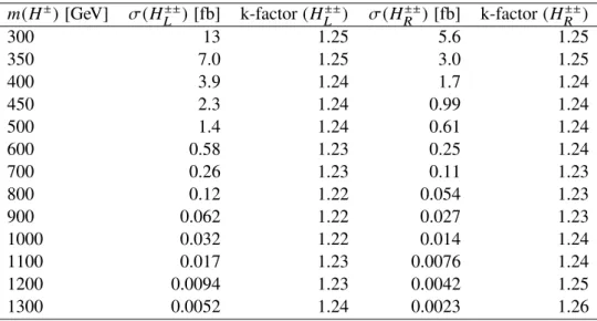
Table 2: NLO cross-sections for pair production of H
L±±H
∓∓Land H
±±RH
∓∓Rwith pp collisions at √
s = 13 TeV.
Calculated by the authors of Ref. [9] using the CTEQ6 PDF [65].
m( H ± ) [GeV] σ (H ±± L ) [fb] k-factor (H L ±± ) σ (H ±± R ) [fb] k-factor (H R ±± )
300 13 1.25 5.6 1.25
350 7.0 1.25 3.0 1.25
400 3.9 1.24 1.7 1.24
450 2.3 1.24 0.99 1.24
500 1.4 1.24 0.61 1.24
600 0.58 1.23 0.25 1.24
700 0.26 1.23 0.11 1.23
800 0.12 1.22 0.054 1.23
900 0.062 1.22 0.027 1.23
1000 0.032 1.22 0.014 1.24
1100 0.017 1.23 0.0076 1.24
1200 0.0094 1.23 0.0042 1.25
1300 0.0052 1.24 0.0023 1.26
The response of the ATLAS detector was simulated using the Geant 4 toolkit [66]. Simulated events were reconstructed using the standard ATLAS software [67] and simulated objects were calibrated using data.
4 Event Selection
Events are required to have at least one reconstructed primary vertex with at least two associated tracks with p T > 400 MeV. Among all the vertices in the event the one with the highest sum of squared transverse momenta of the associated tracks is chosen as the primary vertex.
This analysis classifies leptons in two independent categories called tight and loose, defined specifically for each lepton flavor as described below. All leptons in the analysis regions (see Section 4.1) are required to be selected in the tight category. The estimation of reducible backgrounds is performed using leptons in the loose category. All tracks associated with lepton candidates must have a longitudinal impact parameter with respect to the reconstructed primary vertex, z 0 , satisfying |z 0 sin θ | < 0.5 mm.
Electron candidates are reconstructed using information from the EM calorimeter and ID by matching an
isolated calorimeter energy deposit to an ID track. They are required to have |η | < 2.47, p T > 30 GeV,
and to pass at least the LHLoose identification level based on a multivariate likelihood discriminant [68–
70]. The likelihood discriminant is based on track and calorimeter cluster information. Electron can- didates within the transition region between the barrel and endcap electromagnetic calorimeters (1.37 <
|η | < 1.52) are vetoed. The track associated to the electron candidate must pass the primary vertex re- quirement: the significance of the transverse impact parameter with respect to the beam line (d 0 BL ) must be smaller than 5 (|d BL 0 |/σ (d BL 0 ) < 5). Electron candidates are classified as tight if they additionally pass the LHMedium likelihood based identification level and the isolation criteria described in detail in Ref. [32], based both on calorimeter cluster isolation and track based isolation with a fixed e ffi ciency of selecting prompt electrons of 99% for all values of electron p T and η within the acceptance. Electrons are classified as loose if they fail the LHMedium identification criteria or the isolation criteria.
Muon candidates are formed by combining information from the muon spectrometer and the ID and must satisfy the medium quality criteria described in Ref. [71]. Their transverse momentum is required to be p T > 30 GeV and they must have |η| < 2.5. Muon candidates are classified as tight if the significance of the transverse impact parameter of the associated track satisfies | d 0 BL |/σ (d BL 0 ) < 3.0 and the scalar sum of the p T of tracks, not associated with the muon candidate, within a fixed-size cone radius ∆R = 0.3 around the muon is less than 6% of the muon p T . They are classified as loose muons if they fail the tracking-based isolation and have the significance of the transverse impact parameter satisfy | d 0 BL |/σ (d BL 0 ) < 10.
Jets or particles that originate from the hadronisation of partons are reconstructed by clustering energy deposits in the calorimeter with the anti-k t algorithm [72] with a radius parameter of 0.4, where energy clusters are calibrated at the EM-scale. The majority of pile-up jets are rejected using the ‘jet-vertex- tagger’ (JVT) [73], which is a combination of track-based variables, designed to suppress pile-up jets. For all jets the expected average energy contribution from pile-up is subtracted according to the jet area [74, 75]. Jets are then calibrated as described in Ref. [75]. In this analysis, events containing jets originating from b-quarks are vetoed. These jets are identified as illustrated in [76]. A multivariate discriminant that has a b-jet e ffi ciency of 77% and a rejection factor for jets originating from light quarks (c-quarks) of 40 (20) is used.
After electron identification, jet calibration, and pile-up jet removal, overlaps between objects are re- solved. First, electrons are removed if they share a track with a muon. In a second step, ambiguities between electrons and jets are removed: if the two objects have p
∆φ 2 + ∆η 2 < 0.2 the jet is rejec- ted; if 0.2 < p
∆ φ 2 + ∆ η 2 < 0.4 the electron is rejected. Finally, if the muon and jet are closer than p ∆φ 2 + ∆η 2 < 0.4 the jet is rejected if it has less than 3 tracks; otherwise the muon is rejected.
4.1 Analysis Regions
This analysis relies on the definition of different categories of events, fulfilling different sets of require- ments, called analysis regions. Their purpose is to constrain the free parameters in the fit (Section 6) (control regions), validate the background estimation methods (validation regions) by comparing the background model with data, and compare data with the expected background + signal hypothesis in the fit (signal regions). The regions used in this analysis are summarized in Table 3.
The analysis consists of two, three, and four lepton regions. In two and three lepton regions exactly
one same-charge lepton pair is required and exactly two same-charge lepton pairs are required in four
lepton regions. An exception to the rule is the opposite-charge control region (OCCR) where exactly two
electrons with the opposite charge are required. In all regions events with at least one b-jet are vetoed to
suppress events containing leptons from heavy flavour jets. In regions with more than two leptons, events
are rejected if a Z boson is tagged, i.e. any opposite-charge same-flavour lepton pair is within 10 GeV
of the Z boson mass (81.2 GeV < m(` ± ` ∓ ) < 101.2 GeV). This requirement is applied to reject diboson events featuring a Z boson in the final state, and is inverted in diboson control regions where one or two Z bosons are required. Furthermore, the Z boson veto is removed from four lepton control and validation regions to increase the statistics of the diboson simulated events.
The variable used in the fit for the two and three lepton regions is the invariant mass of the same-charge lepton pair. In the OCCR the invariant mass of the opposite-charge lepton pair is used. A lower bound of 60 GeV on the invariant mass is imposed in all regions since the Z boson MC samples were generated with the requirement that m `` be greater than 60 GeV. In the electron and mixed channels the lower bound is increased to 90 GeV in the three lepton regions and to 130 GeV in the two lepton regions. The motivation for increasing the lower mass bound in regions containing electrons is the data-driven charge mis-identification background correction, where the Z → ee peak is used to measure the charge mis- identification rates (described in detail in Section 5). Di ff erences between data and MC in the di-electron same-charge Z → ee peak were minimized by construction following the methodology described in Section 5, and the Z → ee peak was therefore not used in the fit. In two lepton regions this bound is set to 130 GeV to completely remove the Z peak region. In the three lepton regions, where this e ff ect is not as strong, the bound is relaxed to 90 GeV to increase the available statistics. As the charge mis-identification background is not present in the muon channel, there is no need to increase the lower mass bound there.
In the mixed channel events are further split into two categories: events where the leptons in the same- charge pair have the same flavour (e ± e ± µ ∓ and µ ± µ ± e ∓ ) and events with the opposite-flavour leptons in the same-charge pair (e ± µ ± ` ∓ ).
In order to maximize the sensitivity in two and three lepton signal regions (SR 1P2L and SR 1P3L), additional cuts were imposed on same-charge lepton pairs, regardless of the flavour. These cuts exploit both the boosted topology of the H ±± resonance and the high energy of the decay products: ∆R(` ± ` ± ) <
3.5, p T (` ± ` ± ) > 100 GeV 3 and the scalar sum of the lepton p T is required to be above 300 GeV in these signal regions.
In the four lepton signal region (SR 2P4L), the variable chosen for the final fit is the average of the invariant mass values of the two same-charge pairs. Furthermore, a cut on the variable ∆M/ M, where ¯
∆M = |m ++ − m −− | and ¯ M ≡ m
+++ 2 m
−−is applied to further suppress the background and exploit the fact the H ±± bosons produced in pairs have the same mass. The ∆M/ M ¯ requirement is optimized for di ff erent flavour combinations that take into account the di ff erent lepton resolutions such that the e ffi ciency is comparable for all flavour combinations. The values of the ∆M cut are from 15 GeV to 50 GeV for M ¯ = 200 GeV, 30 GeV to 160 GeV for ¯ M = 500 GeV, and 50 GeV to 500 GeV for ¯ M = 1000 GeV reflecting the better mass resolution of electron final states compared to final states containing muons.
The same-charge validation region (SCVR) is used to validate the data-driven fake background estim- ation and the charge mis-identification e ff ect in the electron channel, the three-lepton validation region (3LVR) is used to validate the SM diboson background and fake events with three reconstructed leptons in total with different proportions across channels, and the four-lepton validation region (4LVR) is used to validate the diboson modelling in the four lepton region. Furthermore, the diboson control region (DBCR) is used to constrain the diboson background yield in each channel separately while the opposite- sign control region (OCCR) is used to constrain the Drell-Yan contribution in the electron channel only.
The four lepton control region (4LCR) is used to constrain the yield of the diboson background in four lepton regions where it has a different composition compared to the three lepton regions.
3
p
T(`
±`
±) stands for the magnitude of the vector sum of p
Tof the two same-charge leptons
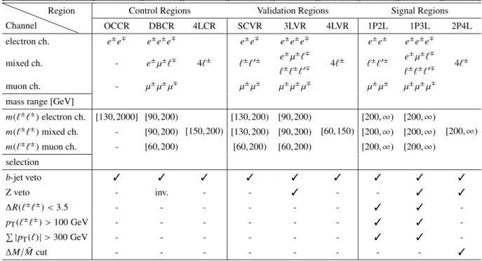
Table 3: Summary of all regions defined in the analysis. The application of a selection requirement is indicated by the check-mark ( 3 ), or by inv. when it is inverted. The 2P4L regions include all lepton flavour combinations. In the three lepton regions `
±`
±`
0∓denotes that same-charge leptons have the same flavour, while the opposite-sign lepton has a di ff erent flavour.
Channel
Region Control Regions Validation Regions Signal Regions
OCCR DBCR 4LCR SCVR 3LVR 4LVR 1P2L 1P3L 2P4L
electron ch. e
±e
∓e
±e
±e
∓4`
±e
±e
∓e
±e
±e
∓4`
±e
±e
±e
±e
±e
∓4`
±mixed ch. - e
±µ
±`
∓`
±`
0±e
±µ
±`
∓`
±`
±`
0∓`
±`
0±e
±µ
±`
∓`
±`
±`
0∓muon ch. - µ
±µ
±µ
∓µ
±µ
±µ
±µ
±µ
∓µ
±µ
±µ
±µ
±µ
∓mass range [GeV]
m(`
±`
±) electron ch. [130, 2000] [90,200)
[150, 200)
[130, 200) [90, 200)
[60, 150)
[200, ∞) [200, ∞)
[200, ∞)
m(`
±`
±) mixed ch. - [90,200) [130, 200) [90, 200) [200, ∞) [200, ∞)
m(`
±`
±) muon ch. - [60,200) [60, 200) [60, 200) [200, ∞) [200, ∞)
selection
b-jet veto 3 3 3 3 3 3 3 3 3
Z veto - inv. - - 3 - - 3 3
∆R(`
±`
±) < 3.5 - - - - - - 3 3 -
p
T(`
±`
±) > 100 GeV - - - - - - 3 3 -
P | p
T(`)| > 300 GeV - - - - - - 3 3 -
∆M/ M ¯ cut - - - - - - - - 3
5 SM Background Composition and Estimation
Prompt SM background in all regions is estimated using MC samples described in Section 3. Prompt light leptons are defined as leptons originating from Z , W, and H bosons or leptons from τ decays where the τ originated from a prompt source (e.g. Z → ττ). MC events containing at least one non-prompt tight or loose lepton are discarded to avoid overlap with the data-driven fake background estimation. Prompt electrons in the remaining simulated events are assigned correction factors to account for the di ff erent charge mis-identification probabilities between data and simulated events.
Electron charge mis-identification is caused predominantly by bremsstrahlung where the emitted photon
can either convert to an electron-positron pair or pass through the ID without directly creating any meas-
urable track. In the first case it can happen that the cluster corresponding to the electron is matched to
the wrong-charge track or that most of the energy is transferred from one track charge to the opposite
through the photon. In the second case the track corresponding to the electron will have very few hits
originating directly from the electron, usually only in the silicon pixel layers, and thus a short lever arm
on its curvature. The electron charge, which is determined from the track curvature, can be incorrectly
determined while the energy of the electron is correct as the emitted photon deposits all of its energy in
the EM calorimeter. Charge mis-identification can also occur due to tracks of highly energetic electrons
where the tracks are approximately straight and it is di ffi cult to determine their curvature. The charge
mis-identification process is not well modelled due to the complexities involved and the need for a very
precise description of the detector material. To correct this, the charge mis-identification probability is
measured in the data and compared to the charge mis-identification probability in the simulation. The
charge mis-identification probability is extracted in a selected Z/γ∗ → ee data sample with a likelihood fit which takes as input the numbers of same-charge (SC) and opposite-charge (OC) electron pairs from the sample (N i j = N SC i j + N OC i j ). The probability of observing N SC i j same-charge events is the Poisson probability:
f ( N SC i j ; λ) = λ N
SCi je −λ
N SC i j ! , (2)
where λ = (P i (1 − P j ) + P j (1 − P i )) N i j is the expected number of same-charge events in bin (i, j) given the charge misidentification probabilities P i and P j and N SC i j is the measured number of same-charge events. The likelihood function is constructed as shown in Equation 3.
− log L (P| N SC , N ) ≈ X
i, j
log(N i j (P i (1 − P j ) + P j (1 − P i ))) N SC i j − N i j (P i (1 − P j ) + P j (1 − P i )). (3)
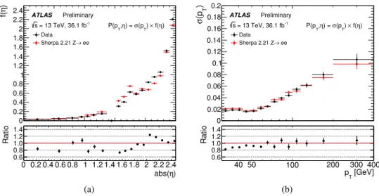
The charge mis-identification probability is parametrized as a function of electron p T and η, P(p T ,η) = f (η ) × σ( p T ), and the binned values of the charge mis-identification probabilities ( f (η ), σ( p T )) are used as free parameters in the likelihood fit. To ensure the proper normalization of P(p T ,η ), the area of the f (η) distribution was set to 1. The charge mis-identification probability is then measured using the same method with a MC Z/γ∗ → ee sample and compared to the data charge mis-identification probability as shown in Figure 2. All prompt electrons in simulated events are assigned a charge re- construction scale factor: P(p T ,η; data)/P(p T ,η; MC) if their charge is incorrectly reconstructed and (1 − P(p T ,η; data)) / (1 − P(p T ,η; MC) if their charge is correctly reconstructed.
) η f(
0 0.2 0.4 0.6 0.8 1 1.2 1.4 1.6 1.8 2 2.2 2.4 ATLAS
Preliminary = 13 TeV, 36.1 fb-1
s ) × f(η)
(pT
) = σ ,η P(pT Data
ee Sherpa 2.21 Z→
) abs( η 0 0.2 0.4 0.6 0.8 1 1.2 1.4 1.6 1.8 2 2.2 2.4
Ratio
0.6 0.8 1.0 1.2 1.4
(a)
)
T(p σ
0 0.02 0.04 0.06 0.08 0.1 0.12 0.14 0.16 0.18 0.2
ATLAS Preliminary = 13 TeV, 36.1 fb-1
s ) × f(η)
(pT
) = σ ,η P(pT Data
ee Sherpa 2.21 Z→
[GeV]
p
T40 50 100 200 300 400
Ratio
0.6 0.8 1.0 1.2 1.4
(b)
Figure 2: Comparison of the charge mis-identification probability P(p
T,η) = σ(p
T) × f (η ) measured from the data and simulation using the likelihood fit in the Z/γ∗ → ee region. The area of the f (η ) distribution is set to 1 (see text for details). Error bars correspond to the uncertainty related to the finite statistics of the Z/γ∗ → ee region.
Plot (a) shows the f (η ) charge mis-identification values, and plot (b) shows the σ(p
T) charge mis-identification
values.
The fake lepton background is estimated in a data-driven approach with the ‘fake factor’ method, similar to the one described in Ref. [27]. Due to the b-jet veto, most of the fake leptons entering the analysis selection are leptons from in-flight decays of mesons inside jets, jets mis-reconstructed as electrons, and photon conversions of final state radiation and initial state radiation photons. The fake factor method estimates the amount of events with fake leptons in analysis regions by extrapolating the information from the yields in the so-called ‘side-band regions’. For each analysis region a corresponding side-band region is defined with exactly the same selection criteria apart from requiring at least one lepton to fail the tight selection criteria. The number of leptons in the analysis regions and their corresponding side-bands is the same (e.g. four tight electrons and three loose plus one tight in the side-band). The ratio of tight to loose leptons is measured in specialized ‘fake enriched regions’ as a function of lepton flavour, p T , and η, and denoted as the ‘fake factor’ (F( p T ,η, flavour)), which is related to the probability for a fake lepton to be reconstructed as a tight one. The definitions of the fake enriched regions used for the electron and muon cases are reported in Table 4. In the measurement, a requirement on the unbalanced momentum in the transverse plane of the event, E T miss , is imposed to reject W + jets events and to further enrich the fake enriched regions in fake leptons. The fake factor method assumes that no prompt leptons appear in the the fake-enriched samples. To account for the fact that this assumption is not fully fulfilled with the imposed cuts, the number of residual prompt electrons in the fake-enriched samples is estimated using MC, and this contribution is subtracted.
The number of events containing at least one fake lepton in the analysis regions, N fake , is estimated from the side-bands by weighting data with the fake factors accordingly to the loose lepton multiplicity of the region:
N fakes =
N
dataL+TX
ev.
( − 1) L + 1
L
Y
l e p.
F l e p. − * . . ,
N
L+TMCX
ev.
( − 1) L + 1
L
Y
l e p.
F l e p. + / / - prompt
(4) where T and L are the number of tight and loose leptons featured in the region, respectively. In Eq. 4, the summation is considered for all events with di ff erent combinations of tight and loose leptons, and the product is considered for only loose leptons in each event. The contribution of prompt leptons in the side-band region is subtracted using simulated events.
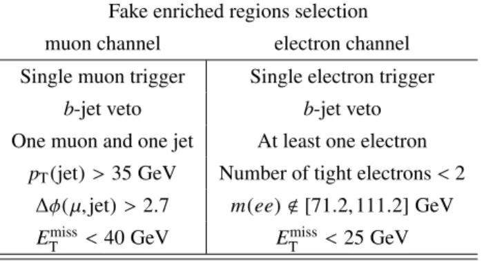
Table 4: Summary of the regions used to measure the proportion of tight and loose leptons for the electron and muon cases.
Fake enriched regions selection muon channel electron channel Single muon trigger Single electron trigger
b-jet veto b-jet veto One muon and one jet At least one electron
p
T(jet) > 35 GeV Number of tight electrons < 2
∆φ(µ, jet) > 2.7 m(ee) < [71.2,111.2] GeV
E
Tmiss< 40 GeV E
Tmiss< 25 GeV
5.1 Systematic Uncertainty of the SM Background Prediction
The cross-sections used to scale the simulated MC events are varied according to the uncertainty in the cross-section calculation, which is 6% for diboson production [77], and 8% to 13% for t¯ t X produc- tion [46], where X is an associated vector boson. The theoretical uncertainty of the Drell-Yan background arises from the PDF eigenvector variations of the nominal PDF set, as well as variations of PDF scale, α S , EW corrections, and photon-induced (PI) corrections. The e ff ect of the PDF choice is also considered by comparing the nominal PDF to several others (CT10NNLO [62], MMHT14 [78], NNPDF3.0 [57], ABM12 [79], HERAPDF2.0 [80], and JR14 [81]) and constructing an envelope by taking the largest de- viations from the nominal choice into account. The most abundant irreducible background, the diboson production, is assigned an additional theoretical uncertainty by comparing the nominal Sherpa 2.2.1 MC sample to the P owheg MC sample. This uncertainty amounts to 5% to 10%.
A significant uncertainty arises from the finite number of simulated events and the finite number of events in the side-band regions. Analysis regions have a very restrictive selection and only a fraction of the initially generated MC events remains in the final selection. Uncertainty due to finite statistics varies from 5% to 40% in the signal regions.
Experimental systematic uncertainties due to different reconstruction, identification, isolation, and trig- ger e ffi ciencies of leptons in data compared to the simulation are estimated by varying the corresponding scale-factors and are less significant compared to the other systematic uncertainties and MC statistical un- certainties. The same is true for experimental systematic uncertainties arising from lepton calibration.
The experimental uncertainty on the charge mis-identification probability of electrons arises from the statistical uncertainty on both the data and the MC Z/γ∗ → ee samples, used to measure the charge mis-identification probabilities, and ranges between 10% and 20% as a function of the electron p T and η.
Possible systematic e ff ects have been investigated by altering the selection requirements on the invariant mass window defined to select Z/γ∗ → ee events for the mis-identification probability measurement.
However, this systematic alteration leads to a negligible effect compared to the statistical one.
The experimental systematic uncertainty on the data-driven fake lepton background estimate is evaluated by varying the nominal fake factor measurement to account for different effects. The E T miss requirement is altered to account for changes in the W + jets composition. The flavour composition of the fakes is invest- igated by adding a recoiling jet requirement for each electron in the electron channel and changing the definition of the recoiling jet in the muon channel. Furthermore, the transverse impact parameter require- ment is varied. Finally, uncertainties in the normalization of simulated samples, used for the subtraction of prompt leptons, are taken into account by altering the total amount of prompt events subtracted from the fake enriched region. This accounts for luminosity, cross-section and uncertainties on the corrections applied to the simulation.
The statistical uncertainty on the fake factors is taken into account by combining it with the total system- atical error in quadrature. The uncertainty ranges between 10% and 20% across all p T and η bins.
The total relative systematic uncertainty after the fit, split into components, is presented in Figure 3.
5.2 Validation of the SM Background Prediction
Dedicated two and three lepton validation regions, defined in Table 3, are used to verify the data-driven
fake lepton estimation in regions as similar as possible to signal regions, while containing a negligible
±
e
±e
±e
±e
±e
±l
±µ
±e
±µ
±µ
±µ
±l
±l
±l
±l
±e
±e
±µ
±e
±µ
±µ
±e
±e
±e
±l
±µ
±e
±µ
±µ
±µ
±l’
±l
±l
±l
±l
±l
±l
±e
±e
±µ
±e
±µ
±µ
±e
±e
±e
±l
±µ
±e
±µ
±µ
±µ
±l’
±l
±l
±l
±l
±l
±l
Relative Uncertainty [%]
1 2 3 10 20 30 40 100
CRs VRs SRs
Total Unc. Stat. Unc.
Theory Fakes
Charge-Flip Yield fit
Exp. Lumi
ATLAS
Preliminary=13 TeV, 36.1 fb-1
s
Figure 3: Relative uncertainties on the total background yield estimation after the fit. ‘Statistical uncertainty’ cor- responds to reducible and irreducible background statistical uncertainties. ‘Yield fit’ corresponds to the uncertainty arising from fitting the yield of diboson and Drell-Yan backgrounds. Individual uncertainties can be correlated, and do not necessarily add up quadratically to the total background uncertainty.
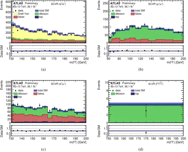
number of signal events. Orthogonality between the signal and validation regions is ensured by requiring that the invariant mass of the same-charge lepton pair m(` ± ` ± ) is less than 200 GeV in the validation regions. Furthermore, diboson modelling and the electron charge mis-identification backgrounds are tested. Each di ff erent background estimation is validated using di ff erent regions, which are defined to be enriched in any given contribution.
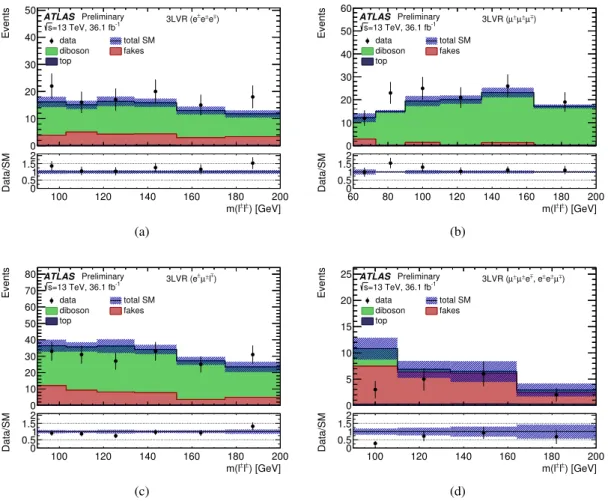
Figure 4 and Figure 5 present all analysis validation regions that test di ff erent backgrounds: same-sign two
lepton validation regions (SCVR) that test the charge mis-identification background and fake background
predictions and three lepton and four lepton validation regions (3LVR and 4LVR, respectively) that test
the diboson modelling.
Events
0 100 200 300 400 500 600 700
800 ATLAS Preliminary
=13 TeV, 36.1 fb-1
s
) e±
SCVR (e±
data total SM
Drell-Yan diboson
fakes top
) [GeV]
l±
m(l±
130 140 150 160 170 180 190 200
Data/SM 00.511.52
(a)
Events
0 50 100 150 200
250 ATLAS Preliminary
=13 TeV, 36.1 fb-1
s
) µ±
µ±
SCVR (
data total SM
diboson fakes top
) [GeV]
l±
m(l±
60 80 100 120 140 160 180 200
Data/SM 00.511.52
(b)
Events
0 20 40 60 80 100 120 140 160 180 200
220 ATLAS Preliminary
=13 TeV, 36.1 fb-1
s
) µ±
SCVR (e±
data total SM
diboson fakes top
) [GeV]
l±
m(l±
130 140 150 160 170 180 190 200
Data/SM 00.511.52
(c)
Events
0 2 4 6 8
10 ATLAS Preliminary
=13 TeV, 36.1 fb-1
s
)±
l±
±l
±l 4LVR (l
data total SM
diboson top
) [GeV]
l±
m(l±
150 155 160 165 170 175 180 185 190 195 200
Data/SM 00.511.52
(d)
Figure 4: Distribution of di-lepton mass for data and SM backgrounds in two and four lepton validation regions. The
systematic bands include all systematic uncertainties post-fit with the correlations between various sources taken
into account for the (a) electron-electron two lepton validation region (SCVR), (b) muon-muon two lepton valid-
ation region (SCVR), (c) electron-muon two lepton validation region (SCVR), and (d) the four lepton validation
region (4LVR).
Events
0 10 20 30 40 50 ATLAS
Preliminary
=13 TeV, 36.1 fb-1
s
)±
e e±
3LVR (e±
data total SM
diboson fakes
top
) [GeV]
l±
m(l±
100 120 140 160 180 200
Data/SM 00.511.52
(a)
Events
0 10 20 30 40 50
60 ATLAS Preliminary
=13 TeV, 36.1 fb-1
s
)±
±µ
±µ 3LVR (µ
data total SM
diboson fakes top
) [GeV]
l±
m(l±
60 80 100 120 140 160 180 200
Data/SM 00.511.52
(b)
Events
0 10 20 30 40 50 60 70
80 ATLAS Preliminary
=13 TeV, 36.1 fb-1
s
)
±
l µ±
3LVR (e±
data total SM
diboson fakes
top
) [GeV]
l±
m(l±
100 120 140 160 180 200
Data/SM 00.511.52
(c)
Events
0 5 10 15 20
25 ATLAS Preliminary
=13 TeV, 36.1 fb-1
s
)±
±µ e , e±
e±
µ±
µ±
3LVR (
data total SM
diboson fakes top
) [GeV]
l±
m(l±
100 120 140 160 180 200
Data/SM 00.511.52
(d)
Figure 5: Distribution of di-lepton mass for data and SM backgrounds in three lepton validation regions. The
systematic bands include all systematic uncertainties post-fit with the correlations between various sources taken
into account for the (a) three electron validation region (VR3L), (b) three muon validation region (VR3L), (c)
VR3L with an electron-muon same-charge pair (e
±µ
±`
∓), and (d) VR3L a same flavour same-charge pair (e
±e
±µ
∓or µ
±µ
±e
∓).
6 Statistical Analysis and Results
The statistical package H ist F itter [82] was used to implement a maximum-likelihood fit of the di-lepton invariant mass distribution in all control and signal regions and the ¯ M distribution in SR 2P4L to ob- tain the observed numbers of signal and background events. The likelihood is the product of a Poisson probability density function describing the observed number of events and, to constrain the nuisance parameters associated with the systematic uncertainties, Gaussian distributions whose widths correspond to the sizes of these uncertainties; Poisson distributions are used instead for MC simulation statistical uncertainties. Furthermore, additional free parameters are introduced for the Drell-Yan and the diboson production background contributions to fit their yield in the analysis regions. The fitted yield parameters are compatible with 1 within the uncertainty. The diboson yield is described by four free parameters each corresponding to a different diboson region: electron channel, muon channel, mixed channel, and the four lepton channel. After the fit, the compatibility between the data and the expected background was assessed and 95% C.L. upper limits were derived on the pp → H ++ H −− cross-section using the CL s method [83] for various branching ratio assumptions.
6.1 Fit Results
The observed and expected yields in all validation, control, and signal regions used in the analysis are presented in Figure 6. No significant excess is observed in any of the signal regions. Correlations between various sources of uncertainties are evaluated and used to estimate the total uncertainty of the SM back- ground prediction. Two and four lepton signal regions are presented in Figure 7 and three lepton signal regions are presented in Figure 8. In the four lepton signal region only a single data event is observed. It is a e + µ + e − µ − event with the same-charge invariant masses of 228 GeV and 207 GeV.
The likelihood fit with two, three, and four lepton control and signal regions was designed to fully exploit the pair production of the H ±± boson with its boosted topology and lepton multiplicity. The fit is very stable across all branching ratio combinations and for Br( H ±± → ` ± ` ± ) = 100% the production cross- section is excluded down to 0.1 fb, which corresponds to 3 − 4 signal events, the theoretical limit of a 95%
exclusion. A few representative cross-section upper limits as a function of H ±± mass are presented in Figure 9 for di ff erent combinations of the light lepton branching ratios. Limits for high electron branching ratio scenarios have a wide one standard deviation discrepancy between 600 GeV and 900 GeV mass due to the two observed events in the corresponding range in the electron channel SR 1P3L (Figure 8(a)).
The final result of the fit is a two-dimensional grid of the lower H ±± mass limit for any combination of light lepton branching ratios that sum to a certain value. The fit was performed for values of Br( H ±± →
` ± ` ± ) from 1% to 5% in 1% intervals, and from 10% to 100% in 10% intervals. Expected limits for the Br (H ±± → ` ± ` ± ) = 100% case are presented in Figure 10 for H L and in Figure 11 for H R . Results of the fit are presented in Figures 12 and 13 for H L ±± and H R ±± , respectively, for the three specific cases of decays only to e ± e ± , µ ± µ ± , and e ± µ ± , along with the minimum limit for each value of Br( H ±± → ` ± ` ± ).
The minimum limit is obtained by taking, for each value of Br (H ±± → ` ± ` ± ), the least stringent limit among limits for any combination of branching ratios that sum to Br( H ±± → ` ± ` ± ). The lower mass limits for these four cases are similar, which indicates that the analysis is almost equally sensitive to each decay channel.
The observed lower mass limits vary from 770 GeV to 870 GeV for H L with Br (H ±± → ` ± ` ± ) = 100%
and are still above 450 GeV for Br (H ±± → ` ± ` ± ) = 10%. For H ±± R the lower mass limits vary from
660 GeV to 760 GeV for Br( H ±± → ` ± ` ± ) = 100% and are above 320 GeV for Br (H ±± → ` ± ` ± ) ≥ 10%.
Events
1
10
−1 10 10
210
310
410
5CRs VRs SRs
ATLAS Preliminary
=13 TeV, 36.1 fb
-1s
data total SM
Drell-Yan diboson
fakes top
±
e
±e
±e
±e
±e
±l
±µ
±e
±µ
±µ
±µ
±l
±l
±l
±l
±e
±e
±µ
±e
±µ
±µ
±e
±e
±e
±l
±µ
±e
±µ
±µ
±µ
±l’
±l
±l
±l
±l
±l
±l
±e
±e
±µ
±e
±µ
±µ
±e
±e
±e
±l
±µ
±e
±µ
±µ
±µ
±l’
±l
±l
±l
±l
±l
±l
Data/SM
0 0.5 1.5 2 1
Figure 6: A summary of all regions used in the analysis. The systematic bands include all systematic uncertainties
post-fit with the correlations between various sources taken into account. `
±`
0±`
∓denotes that the same-charge
leptons have di ff erent flavours and `
±`
±`
0∓denotes that same-charge leptons have the same flavour, while the
opposite-charge lepton has a di ff erent flavour.
Events
0 10 20 30 40 50 60
70 ATLAS Preliminary
=13 TeV, 36.1 fb-1
s
) e±
SR1P2L (e±
data total SM
Drell-Yan diboson
fakes top
)=0.20, Br(X)=0.80 e±
Br(e±
)=450 GeV
±
m(H±
)=0.50, Br(X)=0.50 e±
Br(e±
)=650 GeV
±
m(H±
)=0.50, Br(X)=0.50 e±
Br(e±
)=850 GeV
±
m(H±
) [GeV]
l±
m(l±
300 400 500 1000 2000
Data/SM 00.511.52
(a)
Events
0 2 4 6 8 10 12 14
16 ATLAS Preliminary
=13 TeV, 36.1 fb-1
s
) µ±
µ±
SR1P2L (
data total SM
diboson fakes top
)=0.05, Br(X)=0.95 µ±
µ±
Br(
)=450 GeV
±
m(H±
)=0.50, Br(X)=0.50 µ±
µ±
Br(
)=650 GeV
±
m(H±
)=0.50, Br(X)=0.50 µ±
µ±
Br(
)=850 GeV
±
m(H±
) [GeV]
l±
m(l±
300 400 500 1000 2000
Data/SM 00.511.52
(b)
Events
0 10 20 30 40 50
ATLAS Preliminary
=13 TeV, 36.1 fb-1
s
) µ±
SR1P2L (e±
data total SM
diboson fakes top
)=0.20, Br(X)=0.80 µ±
Br(e±
)=450 GeV
±
m(H±
)=0.50, Br(X)=0.50 µ±
Br(e±
)=650 GeV
±
m(H±
)=0.50, Br(X)=0.50 µ±
Br(e±
)=850 GeV
±
m(H±
) [GeV]
l±
m(l±
300 400 500 1000 2000
Data/SM 00.511.52
(c)
Events
3
10−
−2
10
1
10−
1 10 102
103
104
105 ATLAS Preliminary
=13 TeV, 36.1 fb-1
s
)
±
l
±
±l
±l SR2P4L (l
data total SM
diboson fakes top
)=1.0 µ±
µ±
Br(
)=450 GeV
±
m(H±
)=1.0 µ±
µ±
Br(
)=650 GeV
±
m(H±
)=1.0 µ±
µ±
Br(
)=850 GeV
±
m(H±
) [GeV]
l±
m(l±
200 400 600 800 1000 1200
Data/SM 00.511.52
(d)
Figure 7: Distributions of m(`
±`
±) in representative signal regions. The systematic bands include all systematic
uncertainties post-fit with the correlations between various sources taken into account for the (a) electron-electron
two lepton signal region (SR 1P2L), (b) muon-muon two lepton signal region (SR 1P2L), (c) electron-muon two
lepton signal region (SR 1P2L), and (d) the four lepton signal region (2P4L). Dashed lines correspond to signal
samples, normalized to the theory cross-section, with the H
±±mass and decay modes marked in the legend.
Events
0 2 4 6 8 10 12
14 ATLAS Preliminary
=13 TeV, 36.1 fb-1
s
)±
e e±
SR1P3L (e±
data total SM
diboson fakes
top
)=1.0 e±
Br(e±
)=450 GeV
±
m(H±
)=1.0 e±
Br(e±
)=650 GeV
±
m(H±
)=1.0 e±
Br(e±
)=850 GeV
±
m(H±
) [GeV]
l±
m(l±
300 400 500 1000 2000
Data/SM 00.511.52
(a)
Events
0 2 4 6 8 10 12 14 16 18
20 ATLAS Preliminary
=13 TeV, 36.1 fb-1
s
)±
±µ
±µ SR1P3L (µ
data total SM
diboson top
)=1.0 µ±
µ±
Br(
)=450 GeV
±
m(H±
)=1.0 µ±
µ±
Br(
)=650 GeV
±
m(H±
)=1.0 µ±
µ±
Br(
)=850 GeV
±
m(H±
) [GeV]
l±
m(l±
300 400 500 1000 2000
Data/SM 00.511.52
(b)
Events
0 5 10 15 20 25 30 35 40
45 ATLAS Preliminary
=13 TeV, 36.1 fb-1
s
)
±
l µ±
SR1P3L (e±
data total SM
diboson fakes
top
)=1.0 µ±
Br(e±
)=450 GeV
±
m(H±
)=1.0 µ±
Br(e±
)=650 GeV
±
m(H±
)=1.0 µ±
Br(e±
)=850 GeV
±
m(H±
) [GeV]
l±
m(l±
300 400 500 1000 2000
Data/SM 00.511.52
(c)
Events
0 2 4 6 8 10
12 ATLAS Preliminary
=13 TeV, 36.1 fb-1
s
)±
±µ e , e±
e±
µ±
µ±
SR1P3L (
data total SM
diboson fakes top
)=0.25 µ±
µ±
)=Br(
e±
Br(e±
)=450 GeV
±
m(H±
)=0.50 µ±
µ±
)=Br(
e±
Br(e±
)=650 GeV
±
m(H±
)=0.50 µ±
µ±
)=Br(
e±
Br(e±
)=850 GeV
±
m(H±
) [GeV]
l±
m(l±
200 400 600 800 1000 1200 1400 1600 1800 2000
Data/SM 00.511.52