The ATLAS Collaboration

ATLAS-CONF-2021-017 31March2021

ATLAS CONF Note

ATLAS-CONF-2021-017

March 30, 2021

Search for lepton-flavor-violation in Z -boson decays with τ-leptons with the ATLAS detector

The ATLAS Collaboration

A search for lepton-flavor-violating Z → τe and Z → τµ decays with pp collision data from the ATLAS detector at the LHC is presented. This analysis uses 139 fb

of Run 2 pp collisions at

√ s = 13 TeV and is combined with the results of a similar ATLAS search in the final state in which the τ -lepton decays hadronically using the same data set as well as Run 1 data. The addition of the final state with leptonically decaying τ -leptons significantly improves the sensitivity reach of the previous result. The Z → `τ branching fractions are constrained in this analysis on its own to B(Z → eτ) < 7 . 0 × 10

and B(Z → µτ) < 7 . 2 × 10

at 95%

confidence level. The combination of the two analyses sets the strongest constraints to date:

B(Z → eτ) < 5 . 0 × 10

and B(Z → µτ) < 6 . 5 × 10

at 95% confidence level.

© 2021 CERN for the benefit of the ATLAS Collaboration.

Reproduction of this article or parts of it is allowed as specified in the CC-BY-4.0 license.

Three lepton families (flavors) exist in the Standard Model of particle physics (SM) [1–4], and the number of leptons of each family is conserved in their interactions. Nevertheless, this conservation is not postulated by any fundamental principle of the theory, and neutrino oscillations [5, 6] indicate that processes violating this conservation do occur in nature. According to current knowledge, lepton-flavor-violating (LFV) processes in charged-lepton interactions can occur via neutrino mixing but are too rare to be detected [7].

An observation of these would be an unambiguous sign of physics beyond the SM. LFV processes occur, for example, in theories predicting the existence of heavy neutrinos [8], which may also explain the observed tiny masses and large mixing of the SM neutrinos. In such theories, up to one in 10

Z bosons would undergo an LFV decay involving τ -leptons. In an earlier analysis, the ATLAS experiment at the LHC sets the strongest constraints on the branching fractions ( B ) of the LFV decays of the Z boson involving a τ -lepton by searching for decays in which the τ -lepton decays hadronically [9]. This result was achieved by analyzing proton–proton ( pp ) collision data corresponding to an integrated luminosity of 139 fb

at a center-of-mass energy

√ s = 13 TeV and 20 . 3 fb

at

√ s = 8 TeV. In this search, ATLAS has measured the branching fractions to be B(Z → eτ) < 8 . 1 × 10

and B(Z → µτ) < 9 . 5 × 10

at 95% confidence level (CL), superseding former limits set by the LEP experiments of B(Z → eτ) < 9 . 8 × 10

[10] and B(Z → µτ) < 1 . 2 × 10

[11] at 95% CL.

This Letter presents a corresponding search for Z → `τ decays ( ` = light lepton, e or µ ) in which the τ -leptons decay into electrons or muons ( `τ

channel) using 139 fb

of pp collision data at

√ s = 13 TeV collected by the ATLAS experiment [12]. The search is performed here for the first time at the LHC and is combined with the similar ATLAS search using hadronic τ -lepton decays ( `τ

channel) [9]. The two searches follow similar analysis strategies. Neural network classifiers are used for optimal discrimination of signal from backgrounds and their distributions are employed in a binned maximum-likelihood fit to achieve better sensitivity.

ATLAS1 is a multipurpose particle detector with a forward–backward symmetric cylindrical geometry and a near 4 π coverage in solid angle [12–14]. It consists of an inner tracking detector surrounded by a superconducting solenoid, electromagnetic and hadronic calorimeters, and a muon spectrometer.

This search analyzes pp collision events recorded by the ATLAS experiment using single-electron or single-muon triggers [15–17]. Candidates for electrons [18], muons [19], jets [20–22], and visible decay products of hadronic τ -lepton decays ( τ

) [23, 24] are reconstructed from energy deposits in the calorimeters and charged-particle tracks measured in the inner detector and the muon spectrometer. These candidates are selected following sets of requirements similar to those used in Ref. [9]. Electron candidates are required to pass the Medium likelihood-based identification requirement [18] and have a transverse momentum ( p

) greater than 15 GeV and a pseudorapidity |η| < 1 . 37 or 1 . 52 < |η| < 2 . 47. Muon candidates are required to pass the Medium identification requirement [19] and have a p

larger than 10 GeV and |η | < 2 . 5. Both the electron and muon candidates must satisfy the Tight isolation requirement [18, 19]. Events with exactly one electron and one muon candidate are selected with the requirement that the lepton with higher transverse momentum has p

> 27 GeV. This selection lies above the threshold for constant efficiency of both single-lepton trigger selections. Events with same-flavor lepton pairs are not considered, in order to reduce the background events from Z → `` decays. Events with a leading- p

electron are used in the search for Z → eτ decays ( eτ

channel), while those with a leading- p

muon are used in the search for Z → µτ decays ( µτ

channel), assuming the prompt lepton from the Z -boson decay is the leading one in p

. In the µτ

channel, the electron is required to have the ratio of the p

reconstructed

1ATLAS uses a right-handed coordinate system with its origin at the nominal interaction point (IP) in the center of the detector and thez-axis along the beam pipe. Thex-axis points from the IP to the center of the LHC ring, and they-axis points upward. Cylindrical coordinates(r, φ)are used in the transverse plane,φbeing the azimuthal angle around thez-axis. The pseudorapidity is defined in terms of the polar angleθasη=−ln tan(θ/2).

in the inner tracking detector and in the electromagnetic calorimeter, p

T

(e)/p

T

(e) , to be smaller than 1 . 1 in order to reject Z → µµ events. Opposite charge lepton pair events are analyzed for the search of signal events, while events with same electric charge are used for estimates of background processes.

Quark- or gluon-initiated particle showers (jets) are reconstructed using the anti- k

algorithm [20, 21]

with the radius parameter R = 0 . 4. Jets fulfilling p

> 20 GeV and |η | < 2 . 5 are identified as containing b -hadrons if tagged by a dedicated multivariate algorithm [25]. To ensure the samples of selected events do not overlap with those used in the `τ

channel, events with a τ

candidate are vetoed. The τ

candidates reconstructed from jets with p

> 10 GeV and with one or three associated tracks are selected in |η| < 1 . 37 or 1 . 52 < |η| < 2 . 5. The τ

identification is performed by a recurrent neural network algorithm [23]. A τ

candidate is required to have p

> 25 GeV and to pass the Tight identification selection. The missing transverse momentum ( E

T

) is calculated as the negative vectorial sum of the p

of all fully reconstructed and calibrated physics objects [26, 27]. Additionally, the calculation includes inner detector tracks that originate from the vertex associated with the hard-scattering process but are not associated with any of the reconstructed objects.

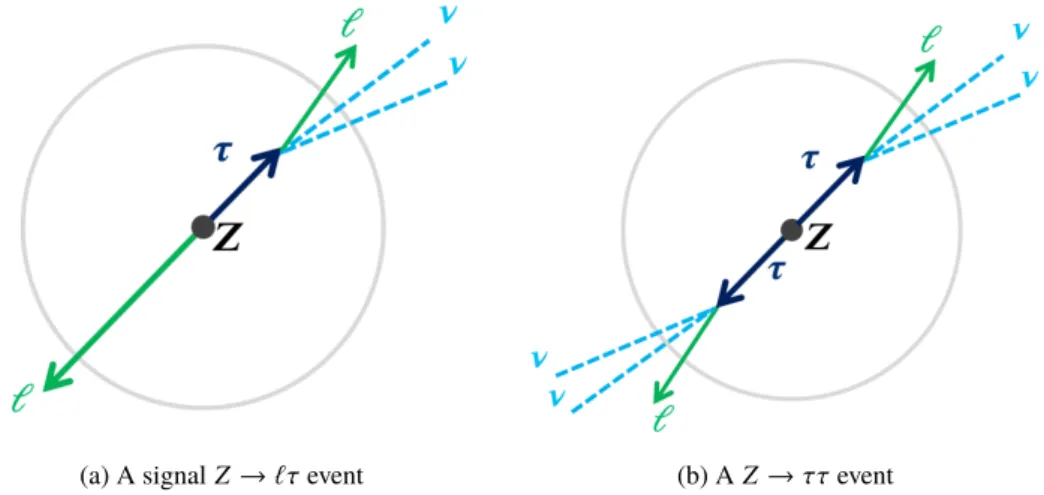
The Z → `τ → ``

+ 2 ν signal events are characterized by their unique final state that has two light leptons with different flavor and opposite electric charge, two collinear neutrinos and an invariant mass of all these particles compatible with the Z -boson mass. These two leptons are emitted approximately back-to-back in the plane transverse to the proton beam direction. Since the τ -lepton is typically boosted due to the large difference between its mass and the mass of its parent Z boson, the two neutrinos from its decay are usually almost collinear with the lepton from the τ -lepton decay. The dominant background contribution is from the lepton-flavor-conserving Z → ττ → ``

+ 4 ν decays, where the two τ -leptons decay leptonically.

Subleading background contributions from other SM processes with final states with two prompt leptons include the decays of a top-antitop-quark pair ( t¯ t ), of two gauge bosons (diboson) or of a Higgs boson.

Finally, small background contributions come from Z → `` decays, where one of the light leptons is misidentified with the wrong flavor; and events with non-prompt leptons. The latter is hereafter referred to as events with ‘fake leptons’ and it includes mostly W(→ `ν) +jets events with misidentified leptons from heavy-flavor quark decays or light-quark-initiated jets. The signal and background events are separated by using a set of selection criteria that define a signal-enhanced sample, referred to as signal region (SR). The selection criteria are listed in Table 1. Three neural network (NN) binary classifiers similar to those used in Ref. [9] are implemented to distinguish signal from background events. An individual NN is trained for Z → ττ , top-quarks and diboson background events, respectively. The NNs are trained on simulated events and each individual NN is optimized to discriminate against a particular background process. The input to these NNs is a mixture of low-level and high-level kinematic variables, following the same strategy as in the `τ

channel [9]. The low-level variables are the momentum components of the reconstructed light leptons and the E

T

. The high-level variables are kinematic properties of the `

– `

– E

T

system, such as the collinear mass m

(`

, `

) , defined as the invariant mass of the `

– `

–2 ν system, where the the vectorial sum of the two neutrinos is assumed to have a momentum that is equal in p

and φ to the measured E

T

and equal in η to the `

momentum. The outputs from the individual NNs (numbers between zero and one) are combined into a final discriminant as shown in Equation 1, hereafter referred to as the ‘combined NN output’:

Combined NN output = 1 − s

1 3

Õ

bkg

( 1 − NN

)

. (1)

Events classified by the NN trained for Z → ττ as background-like are excluded from the SR and used in

a control region to better determine the Z → ττ background in the maximum-likelihood fit. The signal

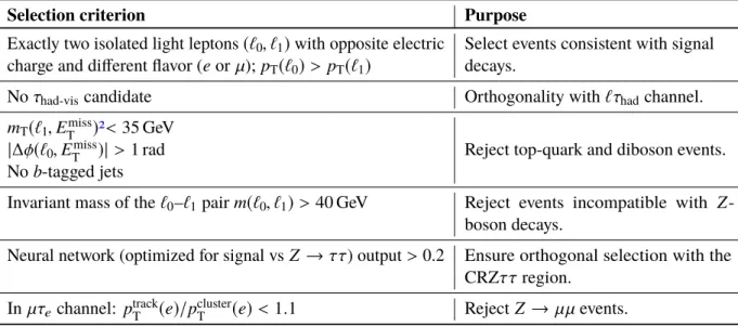
Table 1: Selection criteria for events in the signal region.

Selection criterion Purpose

Exactly two isolated light leptons (`

, `

) with opposite electric charge and different flavor ( e or µ ); p

(`

) > p

(`

)

Select events consistent with signal decays.

No τ

candidate Orthogonality with `τ

channel.

m

(`

, E

T

) 2 < 35 GeV

Reject top-quark and diboson events.

|∆φ(`

, E

T

)| > 1 rad No b -tagged jets

Invariant mass of the `

– `

pair m(`

, `

) > 40 GeV Reject events incompatible with Z - boson decays.

Neural network (optimized for signal vs Z → ττ ) output > 0.2 Ensure orthogonal selection with the CRZ ττ region.

In µτ

channel: p

T

(e)/p

T

(e) < 1 . 1 Reject Z → µµ events.

acceptance in the SR is 19.5% for the eτ

channel and 11.2% for the µτ

channel, as determined from simulated signal samples.

Predictions for signal and background contributions are based partly on Monte Carlo (MC) simulations and partly on estimations from data. Signal and background processes are simulated as in Ref. [9]. The signal events were simulated using Pythia 8 [28] with matrix elements calculated at leading order (LO) in the strong coupling constant. Nominal signal samples were generated with a parity-conserving Z`τ vertex and unpolarized τ -leptons. Scenarios where the decays are maximally parity-violating were considered by reweighting the simulated events using TauSpinner [29], as discussed in Ref. [9]. The Z → ττ background events were simulated with the Sherpa 2.2.1 [30] generator using the NNPDF 3.0 NNLO PDF set [31] and next-to-leading-order (NLO) matrix elements for up to two partons, and LO matrix elements for up to four partons, calculated with the Comix [32] and OpenLoops [33–35] libraries. Background Z → `` events were simulated using the Powheg-Box [36] generator with NLO matrix elements. All MC samples include a detailed simulation of the ATLAS detector with Geant4 [37]. As in Ref. [9], the simulation of Z -boson production is improved through a correction derived from measurements in data. The simulated p

spectra of the Z boson are reweighted to match the unfolded distribution measured by ATLAS in Ref. [38]. The predicted overall yields of signal and Z → ττ events are determined by a binned maximum-likelihood fit to the combined data in the SR and in a control region enhanced in Z → ττ events (CRZ ττ ). This is done by using an unconstrained fit parameter, which eliminates the theoretical uncertainties in the total Z -boson production cross section ( σ

), as well as the experimental uncertainties related to the acceptance of the common ``

final state. The selection criteria for events in the CRZ ττ are the same as those for events in the SR, except that events are required to be classified as Z → ττ -like, that is with an output smaller than 0.2 for the Z → ττ NN and greater than 0.2 for both the top-quark and diboson NNs. In the µτ

channel, a small contribution to the total background originates from Z → µµ events and their predicted yield is based on the measured σ

[39]. The modeling of these events is validated in a region enhanced with Z → µµ events where the subleading muon is mis-reconstructed as an electron. This region has the same selection as the µτ

SR except for the inverse selection on p

T

(e)/p

T

(e) . Based on the observed

2The invariant transverse mass of`andE^miss

T is defined asm_T(`,E^miss

T )= r

2p_T(`)E^miss

T

1−cos

φ_`−φ_Emiss

T .

agreement between data and simulation, a systematic uncertainty of 15% is assigned on the yield of the predicted Z → µµ events in the SR, with no further correction.

Events with fake leptons yield a small but still significant background contribution. In most cases the mis-reconstructed lepton (i.e. the ’fake’ lepton) is the subleading one. These events are estimated from data using a ‘fake-factor method’ similar to the method used in Ref. [9]. The fake factor is defined as the ratio N

fake

/N

fake

, where ‘fake’ indicates events with at least one fake lepton and ‘pass/fail-iso’ indicates whether the subleading lepton passes or fails the isolation requirement. The fake factor is measured in events with pairs of leptons with same electric charge (“SS”). These events are enhanced in W → `ν +jets, which is the dominant contribution of events with fake leptons in the SR. Events in the SS region pass the same event selections as those in the SR besides the charge requirement. The fake factors are measured as functions of the transverse momentum and pseudorapidity of the leptons, separately for eτ

and µτ

events.

The number of events with fake leptons in the SR or in the CRs is estimated by the number of events with the subleading lepton failing the isolation requirement, but otherwise satisfying all other selection criteria for that region, multiplied by the fake factor. This approach is used to model the kinematic properties of the events with fake leptons. The total predicted yields of these events in the SR and CRs are determined by a combined maximum-likelihood fit to data, separately for eτ

and µτ

events. The remaining background processes are estimated using simulations. These backgrounds include events from the production and decay of top quarks [28, 36], pairs of gauge bosons [30, 31] and the Higgs boson [28, 36]. The yield of the events with top-quarks is determined in the maximum-likelihood fit to data via the inclusion of a top-quark control region (“CRTop”). The selection requirements of the CRTop region are the same as the SR besides that at least one b -tagged jet is required. The yields of the remaining processes are normalized to their predicted cross sections. The modeling of the estimated background is validated using events in regions with negligible signal contamination.

A statistical analysis of the selected events is performed to assess the presence of signal events, following the

same method used in Ref. [9]. A simultaneous binned maximum-likelihood fit to the combined NN output

distribution in the SR, the m

(`

, `

) distribution in the CRZ ττ and the event yield in CRTop is used to

constrain uncertainties in the predictions and extract evidence of a possible signal. The fit is performed

independently for the eτ and µτ channels. In order to improve the discrimination between signal and the

events with fake leptons, the events in the SR are further split into two regions based on the transverse

momentum of the subleading- p

lepton. The low- p

SR contains events with p

(`

) < 20 ( 25 ) GeV in the

eτ

( µτ

) channel, while the high- p

SR contains the events above these thresholds. Both SRs are fitted

simultaneously. There are four unconstrained parameters in the fits: the parameter of interest determines

the LFV branching fraction B(Z → `τ) by modifying an arbitrary pre-fit signal yield; µ

determines

σ

times the overall acceptance and reconstruction efficiency of the ``

final state in Z → ττ and signal

events; µ

determines the yield of the top-quarks events; µ

determines the yield of the events with

fake leptons. Constrained parameters are also introduced to account for systematic uncertainties in the

signal and background predictions, as in Ref. [9]. These include uncertainties in simulated events in the

modeling of trigger, reconstruction, identification and isolation efficiencies, as well as energy calibrations

and resolutions of reconstructed objects. No systematic uncertainties on the overall yields are assigned to

events with Z -boson decays, fake leptons or top-quarks as these are determined from data. Uncertainties

on the events with fake leptons include statistical uncertainties due to the size of the data sample used to

measure the fake factors and to model their distributions in the SRs and CRs. Systematic uncertainties on

the events with fake leptons account for: shape differences in the modeling of the combined NN output in

the SS events; differences in the composition of the events with fake leptons between SS events and the

events in the SRs; and uncertainties on the events with prompt leptons failing the isolation requirements

as estimated by simulation. The dominant uncertainties of the search are of statistical nature. Among

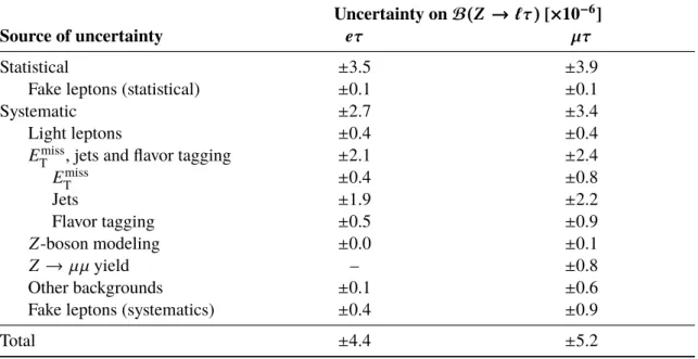
Table 2: Summary of the contributions to the uncertainty on the measuredB(Z →`τ<sub>`</sub>⁰). The uncertainties related to light leptons include those in the trigger, reconstruction, identification and isolation efficiencies, as well as energy calibrations. The uncertainties related to jets andE^miss

T include those in the energy calibration and resolution. The uncertainty on theZ → µµyield is only applicable in theµτchannel. The total systematic uncertainty can differ from the sum in quadrature of the different contributions due to correlations among uncertainties as a result of the likelihood fit to data.

Uncertainty on B(Z → `τ) [×10

]

Source of uncertainty eτ µτ

Statistical ± 3.5 ± 3.9

Fake leptons (statistical) ± 0.1 ± 0.1

Systematic ± 2.7 ± 3.4

Light leptons ± 0.4 ± 0.4

E

T

, jets and flavor tagging ± 2.1 ± 2.4

E

T

± 0.4 ± 0.8

Jets ± 1.9 ± 2.2

Flavor tagging ± 0.5 ± 0.9

Z -boson modeling ± 0.0 ± 0.1

Z → µµ yield – ± 0.8

Other backgrounds ± 0.1 ± 0.6

Fake leptons (systematics) ± 0.4 ± 0.9

Total ± 4.4 ± 5.2

the systematic uncertainties, the dominant ones are those on the jet calibration which enter through the calculation of the E

T

. A summary of the uncertainties and their impact on the LFV branching fraction is given in Table 2.

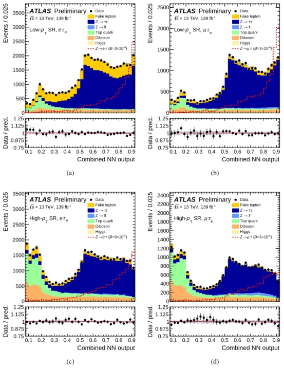
The best-fit predicted and observed distributions of the combined NN output in the low- p

and high- p

SRs are shown in Figure 1 and of the collinear mass in the high- p

SR in Figure 2. The best-fit yield of Z → `τ signal corresponds to the branching fractions B(Z → eτ) = (− 2 . 6 ± 3 . 5 ( stat ) ± 2 . 7 ( syst )) × 10

and B(Z → µτ) = (− 4 . 4 ± 3 . 9 ( stat ) ± 3 . 4 ( syst )) × 10

. The best-fit yields of Z → ττ , top-quarks and events with fake leptons are close to the pre-fit predicted values and are determined with a relative precision of 2%–4%, besides the events with fake leptons in the µτ

channel which have an uncertainty of 30%. As no significant excess of data over the predicted background is observed, a combined fit of the `τ

and `τ

channels is used to set upper limits on B(Z → `τ) . The analysis of the `τ

channel with Run 2 data [9] uses a similar scheme of regions and unconstrained parameters. In the statistical combination, the parameters of interest are correlated. The other unconstrained parameters are uncorrelated as these account either for backgrounds specific to each channel or for different acceptances of the ``

or `τ

final states. Common systematic uncertainties are correlated, besides those related to the jet energy calibrations which are uncorrelated. This conservative correlation scheme was chosen because of different best-fit values for the parameters associated to these uncertainties in the two channels.

However, the fit with correlated jet energy calibration uncertainties yields compatible combined upper

limits. The analysis of the `τ

channel with Run 1 data is combined using the same correlation scheme

as in Ref. [9]. The combined best-fit amount of Z → `τ signal corresponds to the branching fractions

B(Z → eτ) = (− 1 . 4 ± 2 . 5 ( stat ) ± 1 . 8 ( syst )) × 10

and B(Z → µτ) = ( 1 . 7 ± 2 . 2 ( stat ) ± 1 . 6 ( syst )) × 10

.

As no significant deviation from the SM background hypothesis is observed, exclusion limits are set using

obs_x_SR_elmu_low_NN_output_comb__times__1_0__times__1_0

0 500 1000 1500 2000 2500 3000 3500

Events / 0.025

Data Fake lepton

τ τ

→ Z

→ ll Z Top quark Diboson Higgs

-4)

×10

=3 B τ (

→e Z Data Fake lepton

τ τ

→ Z

→ ll Z Top quark Diboson Higgs

-4)

×10

=3 B τ (

→e Z

Preliminary ATLAS

= 13 TeV, 139 fb-1

s

τµ

e SR, pT

Low-

0.1 0.2 0.3 0.4 0.5 0.6 0.7 0.8 0.9 Combined NN output 0.75

0.875 1 1.125 1.25

Data / pred.

(a)

obs_x_SR_muel_low_NN_output_comb__times__1_0__times__1_0

0 500 1000 1500 2000 2500

Events / 0.025

Data Fake lepton

τ τ

→ Z

→ ll Z Top quark Diboson Higgs

-4)

×10

=3 B τ ( µ

→ Z Data Fake lepton

τ τ

→ Z

→ ll Z Top quark Diboson Higgs

-4)

×10

=3 B τ ( µ

→ Z

Preliminary ATLAS

= 13 TeV, 139 fb-1

s

τe

µ SR, pT

Low-

0.1 0.2 0.3 0.4 0.5 0.6 0.7 0.8 0.9 Combined NN output 0.75

0.875 1 1.125 1.25

Data / pred.

(b)

obs_x_SR_elmu_high_NN_output_comb__times__1_0__times__1_0

0 500 1000 1500 2000 2500 3000 3500

Events / 0.025

Data Fake lepton

τ τ

→ Z

→ ll Z Top quark Diboson Higgs

-4)

×10

=3 B τ (

→e Z Data Fake lepton

τ τ

→ Z

→ ll Z Top quark Diboson Higgs

-4)

×10

=3 B τ (

→e Z

Preliminary ATLAS

= 13 TeV, 139 fb-1

s

τµ

e SR, pT

High-

0.1 0.2 0.3 0.4 0.5 0.6 0.7 0.8 0.9 Combined NN output 0.75

0.875 1 1.125 1.25

Data / pred.

(c)

obs_x_SR_muel_high_NN_output_comb__times__1_0__times__1_0

0 200 400 600 800 1000 1200 1400 1600 1800 2000 2200 2400

Events / 0.025

Data Fake lepton

τ τ

→ Z

→ ll Z Top quark Diboson Higgs

-4)

×10

=3 B τ ( µ

→ Z Data Fake lepton

τ τ

→ Z

→ ll Z Top quark Diboson Higgs

-4)

×10

=3 B τ ( µ

→ Z

Preliminary ATLAS

= 13 TeV, 139 fb-1

s

τe

µ SR, pT

High-

0.1 0.2 0.3 0.4 0.5 0.6 0.7 0.8 0.9 Combined NN output 0.75

0.875 1 1.125 1.25

Data / pred.

(d)

Figure 1: Best-fit predicted and observed distributions of the combined NN output in the SRs. The distributions in the low-p_TSR are shown in plots (a) and (b) for theeτ_µandµτ_echannels, respectively, while plots (c) and (d) show the distributions in the high-p_TSR for theeτ_µandµτ_echannels, respectively. The expected signal, normalized to the arbitraryB(Z →`τ)=3×10⁻⁴for visualization, is shown as a dashed red histogram in each plot. In the panel below each plot, the ratio of the observed yield (dots) and the best-fit background-plus-signal yield (solid red line) to the best-fit background yield are shown. The hatched error bands represent a one standard deviation of the combined statistical and systematic uncertainties. The first and last bins in each plot include underflow and overflow events, respectively.

obs_x_SR_elmu_high_el_mu_mcoll__times__1_0__times__1_0

0 2000 4000 6000 8000 10000 12000 14000 16000 18000

Events / 10 GeV

Data Fake lepton

τ τ

→ Z

→ ll Z Top quark Diboson Higgs

-4)

×10

=3 B τ (

→e Z Data Fake lepton

τ τ

→ Z

→ ll Z Top quark Diboson Higgs

-4)

×10

=3 B τ (

→e Z

Preliminary ATLAS

= 13 TeV, 139 fb-1

s

τµ

e SR, pT

High-

60 70 80 90 100 110 120 130 140 150 160 ) [GeV]

e µ,

coll( m 0.75

0.875 1 1.125 1.25

Data / pred.

(a)

obs_x_SR_muel_high_mu_el_mcoll__times__1_0__times__1_0

0 2000 4000 6000 8000 10000

Events / 10 GeV

Data Fake lepton

τ τ

→ Z

→ ll Z Top quark Diboson Higgs

-4)

×10

=3 B τ ( µ

→ Z Data Fake lepton

τ τ

→ Z

→ ll Z Top quark Diboson Higgs

-4)

×10

=3 B τ ( µ

→ Z

Preliminary ATLAS

= 13 TeV, 139 fb-1

s

τe

µ SR, pT

High-

60 70 80 90 100 110 120 130 140 150 160 ) [GeV]

µ , e

coll( m 0.75

0.875 1 1.125 1.25

Data / pred.

(b)

Figure 2: Best-fit predicted and observed distributions of the the collinear mass in the high-p_TSRs. Plots (a) and (b) show the distributions for theeτ_µandµτ_echannels, respectively. The expected signal, normalized to the arbitrary B(Z →`τ)=3×10⁻⁴for visualization, is shown as a dashed red histogram in each plot. In the panel below each plot, the ratio of the observed yield (dots) and the best-fit background-plus-signal yield (solid red line) to the best-fit background yield are shown. The hatched error bands represent a one standard deviation of the combined statistical and systematic uncertainties. The first and last bins in each plot include underflow and overflow events, respectively.

Table 3: Observed and expected (median) upper limits on the signal branching fraction at 95% CL, in different τ-polarization scenarios.

Observed (expected) upper limit on B(Z → `τ) [×10

]

Final state, polarization assumption eτ µτ

`τ

Run 1 + Run 2, unpolarized τ [9] 8.1 (8.1) 9.5 (6.1)

`τ

Run 2, left-handed τ [9] 8.2 (8.6) 9.5 (6.7)

`τ

Run 2, right-handed τ [9] 7.8 (7.6) 10 (5.8)

`τ

Run 2, unpolarized τ 7.0 (8.9) 7.2 (10)

`τ

Run 2, left-handed τ 5.9 (7.5) 5.7 (8.5)

`τ

Run 2, right-handed τ 8.4 (11) 9.2 (13)

Combined `τ Run 1 + Run 2, unpolarized τ 5.0 (6.0) 6.5 (5.3)

Combined `τ Run 2, left-handed τ 4.5 (5.7) 5.6 (5.3)

Combined `τ Run 2, right-handed τ 5.4 (6.2) 7.7 (5.3)

the CL

method [40]. The upper limits are shown in Table 3 for LFV decays with different assumptions about the τ -polarization state. In the scenario where the τ -leptons are unpolarized, the observed upper limits at 95% CL on B(Z → eτ) and B(Z → µτ) are 5 . 0 × 10

and 6 . 5 × 10

, respectively.

In conclusion, in this Letter the `τ

channel has been analyzed in the search for Z → `τ decays for the first

time at the LHC. This channel yields a sensitivity similar to the `τ

channel. With the combined results

of the two channels, the ATLAS experiment sets the most stringent constraints on LFV Z -boson decays

involving τ -leptons to date. The precision of these results is mainly limited by statistical uncertainties.

Appendix

(a) A signalZ →`τevent (b) AZ→ττevent

Figure 3: Schematic representation of the typical topology of an event selected in the SR, as seen in the plane transverse to the beam line. The green arrows represent reconstructed light leptons (`). The light blue dashed lines represent neutrinos that escape detection and are reconstructed as (part of) the missing transverse momentum of the event.

Table 4: Input variables for the neural network classifiers. The first six variables are the low-level variables, which are measured in the boosted and rotated frame as described in the text. The last three variables are the high-level variables, which are measured in the laboratory frame.

Variable Description

p

(`

) z -component of the leading- p

lepton’s momentum.

E(`

) Energy of the leading- p

lepton.

p

(`

) x -component of the sub-leading- p

lepton’s momentum.

p

(`

) z -component of the sub-leading- p

lepton’s momentum.

E(`

) Energy of the sub-leading- p

lepton.

E

T

The missing transverse momentum.

m(e, µ) The invariant mass of the e – µ system.

m

(e, µ) The collinear mass: the invariant mass of the e – µ – ν system, where the ν is assumed to have a momentum that is equal in the transverse plane to the measured E

T

and collinear in η with the sub-leading- p

lepton.

∆ α A kinematic discriminant sensitive to the different fractions of τ -lepton four-momentum

carried by neutrinos in signal and background [41].

0 20 40 60 80 100 120 140

Events / 0.05

Simulation Preliminary ATLAS

= 13 TeV, 139 fb-1

s

polarization τ

Unpolarized Left-handed Right-handed

τµ

e SR, pT

High-

0.1 0.2 0.3 0.4 0.5 0.6 0.7 0.8 0.9 Combined NN output 0

0.5 1 1.5 2

Ratio

(a)

0 10 20 30 40 50 60

Events / 0.05

Simulation Preliminary ATLAS

= 13 TeV, 139 fb-1

s

polarization τ

Unpolarized Left-handed Right-handed

τe

µ SR, pT

High-

0.1 0.2 0.3 0.4 0.5 0.6 0.7 0.8 0.9 Combined NN output 0

0.5 1 1.5 2

Ratio

(b)

0 20 40 60 80 100 120 140 160

Events / 0.05

Simulation Preliminary ATLAS

= 13 TeV, 139 fb-1

s

polarization τ

Unpolarized Left-handed Right-handed

τµ

e SR, pT

Low-

0.1 0.2 0.3 0.4 0.5 0.6 0.7 0.8 0.9 Combined NN output 0

0.5 1 1.5 2

Ratio

(c)

0 20 40 60 80 100 120 140

Events / 0.05

Simulation Preliminary ATLAS

= 13 TeV, 139 fb-1

s

polarization τ

Unpolarized Left-handed Right-handed

τe

µ SR, pT

Low-

0.1 0.2 0.3 0.4 0.5 0.6 0.7 0.8 0.9 Combined NN output 0

0.5 1 1.5 2

Ratio

(d)

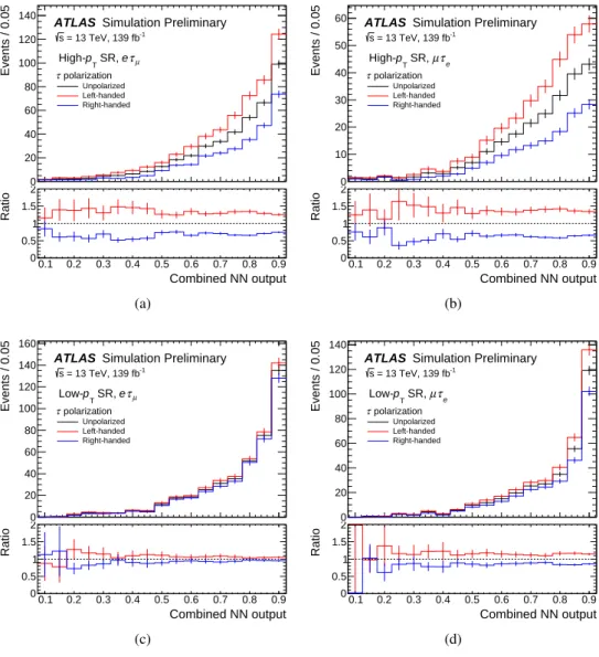
Figure 4: Combined NN output distributions in the high-p_TSR in the (a)eτ_µand (b)µτ_echannels and in the low-p_T SR in the (c)eτ_µand (d)µτ_echannels before and after theτpolarization reweighting. The ratios of the reweighted distributions to the original distributions (corresponding to unpolarizedτ) are shown in the bottom panels. The signal is normalized toB(Z →`τ)=10⁻⁵. The error bars represent the MC statistical uncertainties. The last bin in each plot includes overflow events.

obs_x_CRZtt_elmu_el_mu_mcoll__times__1_0

0 5000 10000 15000 20000 25000

Events / 10 GeV

Data Fake lepton

τ τ

→ Z

→ ll Z Top quark Diboson Higgs

-4)

×10

=3 B τ (

→e Z Data Fake lepton

τ τ

→ Z

→ ll Z Top quark Diboson Higgs

-4)

×10

=3 B τ (

→e Z

Preliminary ATLAS

= 13 TeV, 139 fb-1

s

τµ

e CR, τ τ Z

50 55 60 65 70 75 80 85 90

) [GeV]

e µ,

coll( m 0.75

0.875 1 1.125 1.25

Data / pred.

(a)

obs_x_CRZtt_muel_mu_el_mcoll__times__1_0

0 2000 4000 6000 8000 10000 12000 14000 16000 18000 20000

Events / 10 GeV

Data Fake lepton

τ τ

→ Z

→ ll Z Top quark Diboson Higgs

-4)

×10

=3 B τ ( µ

→ Z Data Fake lepton

τ τ

→ Z

→ ll Z Top quark Diboson Higgs

-4)

×10

=3 B τ ( µ

→ Z

Preliminary ATLAS

= 13 TeV, 139 fb-1

s

τe

µ CR, τ τ Z

50 55 60 65 70 75 80 85 90

) [GeV]

µ , e

coll( m 0.75

0.875 1 1.125 1.25

Data / pred.

(b)

obs_x_CRZtt_elmu_NN_output_comb__times__1_0__times__1_0__times__1_0

0 1000 2000 3000 4000 5000 6000

Events / 0.025

Data Fake lepton

τ τ

→ Z

→ ll Z Top quark Diboson Higgs

-4)

×10

=3 B τ (

→e Z Data Fake lepton

τ τ

→ Z

→ ll Z Top quark Diboson Higgs

-4)

×10

=3 B τ (

→e Z

Preliminary ATLAS

= 13 TeV, 139 fb-1

s

τµ

e CR, τ τ Z

0.1 0.15 0.2 0.25 0.3 0.35 0.4 0.45 0.5 0.55 Combined NN output 0.75

0.875 1 1.125 1.25

Data / pred.

(c)

obs_x_CRZtt_muel_NN_output_comb__times__1_0__times__1_0__times__1_0

0 500 1000 1500 2000 2500 3000 3500 4000

Events / 0.025

Data Fake lepton

τ τ

→ Z

→ ll Z Top quark Diboson Higgs

-4)

×10

=3 B τ ( µ

→ Z Data Fake lepton

τ τ

→ Z

→ ll Z Top quark Diboson Higgs

-4)

×10

=3 B τ ( µ

→ Z

Preliminary ATLAS

= 13 TeV, 139 fb-1

s

τe

µ CR, τ τ Z

0.1 0.15 0.2 0.25 0.3 0.35 0.4 0.45 0.5 0.55 Combined NN output 0.75

0.875 1 1.125 1.25

Data / pred.

(d)

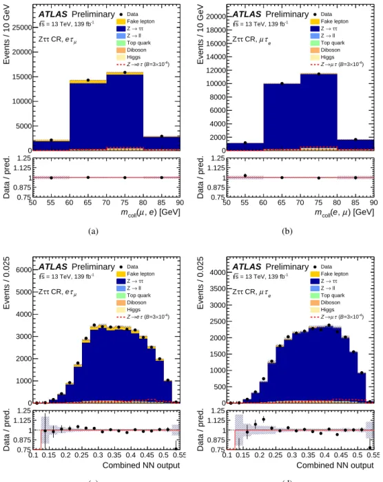
Figure 5: Best-fit predicted and observed distributions used in the CRZττ. Collinear mass distributionsm_coll(e, µ)for the (a)eτ_µ and (b)µτ_echannel. Combined NN output for the (c)eτ_µand (d) µτ_echannel. The expected signal, normalized to the arbitraryB(Z →`τ)=3×10⁻⁴for visualization, is shown as a dashed red histogram in each plot.

In the panel below each plot, the ratio of the observed yield (dots) and the best-fit background-plus-signal yield (solid red line) to the best-fit background yield are shown. The hatched error bands represent a one standard deviation of the combined statistical and systematic uncertainties. The last bin in each plot includes overflow events.

obs_x_SR_elmu_high_electrons_pt_0___times__1_0

0 2000 4000 6000 8000 10000 12000 14000 16000

Events / 5 GeV

Data Fake lepton

τ τ

→ Z

→ ll Z Top quark Diboson Higgs

-4)

×10

=3 B τ (

→e Z Data Fake lepton

τ τ

→ Z

→ ll Z Top quark Diboson Higgs

-4)

×10

=3 B τ (

→e Z

Preliminary ATLAS

= 13 TeV, 139 fb-1

s

τµ

e SR, pT

High-

30 40 50 60 70 80

) [GeV]

e

T( p 0.75

0.875 1 1.125 1.25

Data / pred.

(a)

obs_x_SR_muel_high_muons_pt_0___times__1_0

0 1000 2000 3000 4000 5000 6000 7000 8000 9000

Events / 5 GeV

Data Fake lepton

τ τ

→ Z

→ ll Z Top quark Diboson Higgs

-4)

×10

=3 B τ ( µ

→ Z Data Fake lepton

τ τ

→ Z

→ ll Z Top quark Diboson Higgs

-4)

×10

=3 B τ ( µ

→ Z

Preliminary ATLAS

= 13 TeV, 139 fb-1

s

τe

µ SR, pT

High-

30 40 50 60 70 80

) [GeV]

µ

T( p 0.75

0.875 1 1.125 1.25

Data / pred.

(b)

obs_x_SR_elmu_low_met_et

0 2000 4000 6000 8000 10000 12000

Events / 5 GeV

Data Fake lepton

τ τ

→ Z

→ ll Z Top quark Diboson Higgs

-4)

×10

=3 B τ (

→e Z Data Fake lepton

τ τ

→ Z

→ ll Z Top quark Diboson Higgs

-4)

×10

=3 B τ (

→e Z

Preliminary ATLAS

= 13 TeV, 139 fb-1

s

τµ

e SR, pT

Low-

0 10 20 30 40 50 60 70 80

[GeV]

miss

ET 0.75

0.875 1 1.125 1.25

Data / pred.

(c)

obs_x_SR_muel_low_met_et

0 1000 2000 3000 4000 5000 6000 7000

Events / 5 GeV

Data Fake lepton

τ τ

→ Z

→ ll Z Top quark Diboson Higgs

-4)

×10

=3 B τ ( µ

→ Z Data Fake lepton

τ τ

→ Z

→ ll Z Top quark Diboson Higgs

-4)

×10

=3 B τ ( µ

→ Z

Preliminary ATLAS

= 13 TeV, 139 fb-1

s

τe

µ SR, pT

Low-

0 10 20 30 40 50 60 70 80

[GeV]

miss

ET 0.75

0.875 1 1.125 1.25

Data / pred.

(d)

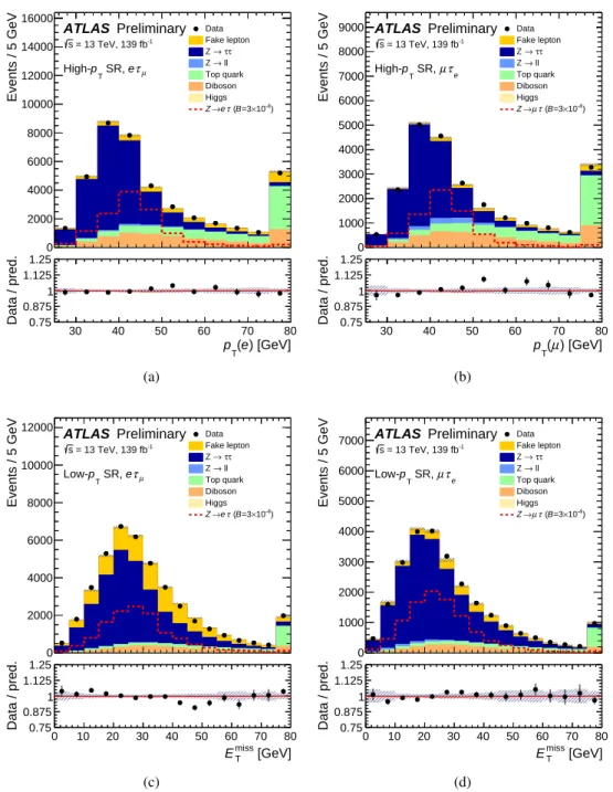
Figure 6: Best-fit predicted and observed distributions in SRs. Leading leptonp_Tin the high-p_TSR for the (a)eτ_µ and (b)µτ_echannel. E^miss

T in the low-p_TSR for the (c)eτ_µand (d)µτ_echannel. The expected signal, normalized to the arbitraryB(Z →`τ)=3×10⁻⁴for visualization, is shown as a dashed red histogram in each plot. In the panel below each plot, the ratio of the observed yield (dots) and the best-fit background-plus-signal yield (solid red line) to the best-fit background yield are shown. The hatched error bands represent a one standard deviation of the combined statistical and systematic uncertainties. The last bin in each plot includes overflow events.

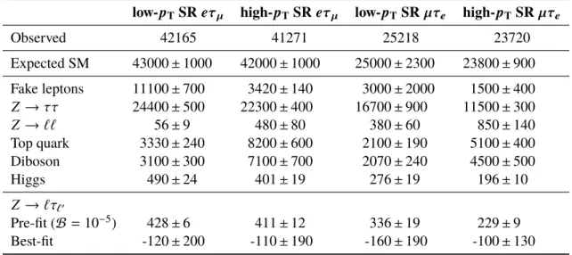
Table 5: Observed number of events and best-fit expected background and signal yields in the SRs of theeτ_µandµτ_e channels. The events in the low-p_Tand high-p_TSR are fitted simultaneously. The uncertainties include both the statistical and systematic contributions.

low-p

SR eτ

high- p

SR eτ

low-p

SR µτ

high- p

SR µτ

Observed 42165 41271 25218 23720

Expected SM 43000 ± 1000 42000 ± 1000 25000 ± 2300 23800 ± 900 Fake leptons 11100 ± 700 3420 ± 140 3000 ± 2000 1500 ± 400

Z → ττ 24400 ± 500 22300 ± 400 16700 ± 900 11500 ± 300

Z → `` 56 ± 9 480 ± 80 380 ± 60 850 ± 140

Top quark 3330 ± 240 8200 ± 600 2100 ± 190 5100 ± 400

Diboson 3100 ± 300 7100 ± 700 2070 ± 240 4500 ± 500

Higgs 490 ± 24 401 ± 19 276 ± 19 196 ± 10

Z → `τ

Pre-fit ( B = 10

) 428 ± 6 411 ± 12 336 ± 19 229 ± 9

Best-fit -120 ± 200 -110 ± 190 -160 ± 190 -100 ± 130

Table 6: Summary of the uncertainties and their impacts on the measuredB(Z →`τ)for the combined fit based on Run 2 data for the`τ_hadand`τ<sub>`</sub>⁰ channels. The statistical uncertainties include those in the determination of the yields of the events with fake leptons. The uncertainties related to light leptons include those in the trigger, reconstruction, identification and isolation efficiencies, as well as energy calibrations. The uncertainties related to jets andE^miss

T include those in the energy calibration and resolution.

Uncertainty on B( Z → `τ ) [×10

]

Source of uncertainty eτ µτ

Statistical ± 2.5 ± 2.3

Systematic ± 1.8 ± 1.2

τ

candidates ± 1.1 ± 1.1

Light leptons ± 0.4 ± 0.2

E

T

, jets and flavor tagging ± 1.1 ± 0.7

E

T

± 0.2 ± 0.2

Jets ± 1.0 ± 0.7

Flavor tagging ± 0.3 ± 0.3

Z -boson modeling ± 0.6 ± 0.1

Z → `` ± 0.1 ± 0.2

Luminosity ± 0.2 ± 0.0

Other minor backgrounds ± 0.4 ± 0.3

Fake leptons ± 0.2 ± 0.3

Total ± 3.0 ± 2.8

References

[1] S. Glashow, Partial-symmetries of weak interactions, Nucl. Phys. 22 (1961) 579 (cit. on p. 2).

[2] S. Weinberg, A Model of Leptons, Phys. Rev. Lett. 19 (1967) 1264 (cit. on p. 2).

[3] A. Salam, “Weak and Electromagnetic Interactions,” Elementary particle theory: Relativistic groups and analyticity. Proceedings of the Eighth Nobel Symposium, 1968 367 (cit. on p. 2).

[4] G. ’t Hooft and M. Veltman, Regularization and renormalization of gauge fields, Nucl. Phys. B 44 (1972) 189 (cit. on p. 2).

[5] Super-Kamiokande Collaboration, Evidence for Oscillation of Atmospheric Neutrinos, Phys. Rev. Lett. 81 (1998) 1562 (cit. on p. 2).

[6] SNO Collaboration, Direct Evidence for Neutrino Flavor Transformation from Neutral-Current Interactions in the Sudbury Neutrino Observatory, Phys. Rev. Lett. 89 (2002) 011301 (cit. on p. 2).

[7] J. I. Illana, M. Jack, and T. Riemann, “Predictions for Z → µτ and related reactions,”

2nd Workshop of the 2nd Joint ECFA / DESY Study on Physics and Detectors for a Linear Electron Positron Collider, 1999 490, arXiv: hep-ph/0001273 (cit. on p. 2).

[8] J. I. Illana and T. Riemann, Charged lepton flavor violation from massive neutrinos in Z decays, Phys. Rev. D 63 (2001) 053004 (cit. on p. 2).

[9] ATLAS Collaboration, Charged-lepton-flavour violation at the LHC: a search for Z → eτ/µτ decays with the ATLAS detector, (2020), arXiv: 2010.02566 [hep-ex] (cit. on pp. 2–6, 8).

[10] OPAL Collaboration, A search for lepton flavor violating Z

decays, Z. Phys. C 67 (1995) 555 (cit. on p. 2).

[11] DELPHI Collaboration, Search for lepton flavor number violating Z

decays, Z. Phys. C 73 (1997) 243 (cit. on p. 2).

[12] ATLAS Collaboration, The ATLAS Experiment at the CERN Large Hadron Collider, JINST 3 (2008) S08003 (cit. on p. 2).

[13] ATLAS Collaboration, ATLAS Insertable B-Layer Technical Design Report, ATLAS-TDR-19; CERN-LHCC-2010-013, 2010,

url: https://cds.cern.ch/record/1291633 (cit. on p. 2).

[14] ATLAS Collaboration, Production and integration of the ATLAS Insertable B-Layer, JINST 13 (2018) T05008, arXiv: 1803.00844 [physics.ins-det] (cit. on p. 2).

[15] ATLAS Collaboration, Performance of the ATLAS trigger system in 2015, Eur. Phys. J. C 77 (2017) 317, arXiv: 1611.09661 [hep-ex] (cit. on p. 2).

[16] ATLAS Collaboration, Performance of electron and photon triggers in ATLAS during LHC Run 2, Eur. Phys. J. C 80 (2020) 47, arXiv: 1909.00761 [hep-ex] (cit. on p. 2).

[17] ATLAS Collaboration, Performance of the ATLAS muon triggers in Run 2, JINST 15 (2020) P09015, arXiv: 2004.13447 [hep-ex] (cit. on p. 2).

[18] ATLAS Collaboration, Electron and photon performance measurements with the ATLAS detector using the 2015–2017 LHC proton–proton collision data, JINST 14 (2019) P12006,

arXiv: 1908.00005 [hep-ex] (cit. on p. 2).