ATLAS-CONF-2014-002 11February2014
ATLAS NOTE
ATLAS-CONF-2014-002
February 10, 2014
The ATLAS transverse-momentum trigger performance at the LHC in 2011
The ATLAS Collaboration
Abstract
The transverse momentum triggers of the ATLAS experiment at the CERN Large Hadron Collider are designed to select collision events with non-interacting particles passing through the detector and events with a large amount of outgoing momentum transverse to the beam axis. These triggers use global sums over the full calorimeter so are sensitive to measurement fluctuations and systematic changes anywhere in the detector. During the 2011 data-taking period, the LHC beam conditions for proton-proton collisions went through considerable evolution, starting with an average number of interactions per bunch crossing in a run,
hµi, of about 3, increasing to typical values of 7 to 15, and even including one run with
hµiof about 30. These changes were accompanied by changes in the bunch structure, including the number of filled bunches, how these were spaced, and the intensity of individual bunches.
An increase in
µresults in an increase of both the average energy deposit in the calorimeter and the energy-measurement fluctuations. Changes in beam conditions in turn necessitated changes in the calorimeter noise-suppression schemes used at various trigger levels. Trans- verse momentum distributions and trigger rates were impacted by all of these changes. This note contains a description of the transverse momentum triggers, the challenges faced in the 2011 data-taking period, the strategies used to deal with changes in the beam and detector, and characterization of the trigger performance in 2011. Even under these conditions, the trigger behavior was close to what was expected and allowed robust collection of data used for physics studies.
©Copyright 2014 CERN for the benefit of the ATLAS Collaboration.
Reproduction of this article or parts of it is allowed as specified in the CC-BY-3.0 license.
1 Introduction
In 2011, the ATLAS Experiment [1] at the CERN Large Hadron Collider (LHC) collected 5.25 fb
−1of data for proton-proton collisions at
√s
=7 TeV and 158
µb−1of data for lead-lead collisions with nucleon-pair center of mass energy
√s
NN =2.76 TeV (prior to any data quality cuts). The goal of the ATLAS missing transverse momentum (E
missT) triggers [2, 3] is to select events with an imbalance in the total measured momentum due to the presence of particles invisible to the detector. These include neutrinos, which are produced in the decay chains of Standard-Model particles such as the W and Z, heavy quarks, and the Higgs boson. Such events can also arise from the presence of non-interacting particles predicted by theories Beyond the Standard Model, such as the lightest SUSY particle. In o
ffline analysis the full detector information can be accessed to get an optimum determination of E
Tmiss. At the trigger level, however, both computing time and access to the detector information is limited. In 2011, the ATLAS trigger used calorimeter cell positions and the energies they measured in an event to obtain a good approximation of the measurable missing total transverse momentum in that event. In this approach, the components of the missing transverse momentum vector,
EmissT
, are defined as
6Ex=−ΣiE
isin
θicos
φiand
6Ey=−ΣiE
isin
θisin
φiwhere the sum is over all calorimeter cells i (or grouping of cells i, depending on the granularity of information available at the trigger level in which the calculation is being done), E
iis the energy measured in cell i,
θiis the angle between the cell i position unit vector
~vi(which points from the center of the ATLAS detector to cell i) and the beam axis, and
φiis the angle between the projection of
~vionto the plane perpendicular to the beam axis and the horizontal axis pointing towards the center of the LHC ring. E
missTis defined as
q
(6E
x)
2+(6E
y)
2and is used to select candidate events for further study.
The scalar sum of the calorimeter cell energies times the projection of their position unit vectors onto the plane perpendicular to the beam axis,
ΣE
T = ΣiE
isin
θi, can be used as an indication of a hard scatter having taken place, and is therefore also potentially a useful quantity with which to detect interesting events.
E
missTand
ΣE
Tare both determined by summing over the full calorimeter. Even in events where there are no non-interacting particles produced, imperfect calorimeter resolution will give rise to non-zero values of E
missT. Greater energy deposit in the calorimeters results in larger
ΣE
Tand larger calorimeter fluctuations, yielding more events passing
ΣE
Tand E
Tmisstrigger thresholds. For large bunch densi- ties, multiple proton-proton interactions occur in a single bunch crossing, each depositing energy in the calorimeters. LHC beam luminosity for proton-proton collisions increased during 2011, so that
hµi, theaverage over a fill of the Poisson mean number
µof beam interactions per bunch crossing, typically varied from about 7 to 15, but started at about 3 in early 2011 and went as high as 30 in one fill (though the latter had beam conditions very di
fferent than was typical for 2011). As this “pileup” contribution to the calorimeter energy measurement increases, in the absence of other modifications to mitigate this ef- fect, the E
missTtrigger thresholds must be raised or prescales (the inverse of the fraction of passing events retained) increased to keep trigger rates below the maximum that the system can record. A new type of trigger, using missing transverse momentum significance (XS), was therefore introduced in 2011 to accept some events with signal E
Tmissbelow that of the E
Tmisstrigger threshold. In XS triggers, the E
missTresolution in an event is parameterized as a function of
ΣE
Tin that event, and the trigger criterion is the ratio of E
missTto its resolution.
The following sections describe the transverse momentum triggers and assess their performance in
the 2011 data-taking period. The largest fraction of LHC proton-proton events are collisions without
large momentum transfer, followed by two-jet events from hard parton scatters. The E
missTtrigger rate is
dominated by mismeasurement of these events, even though they do not have real E
missT. Trigger behav-
ior for event samples selected with minimal requirements is therefore one aspect of trigger performance
studied here. Samples rich in W decays to lepton and neutrino events are used to determine the e
fficiency
of the trigger to select events with real invisible particles. Other characterizations of performance include how well the quantities calculated by the triggers match the respective o
ffline quantities, how well the trigger performance matches what is expected from simulations, and how pileup affects the signal effi- ciency and background rejection. These triggers were stable and robust, even in the highest 2011 pileup conditions, though some threshold and prescale adjustments had to be done for the higher luminosities.
The 2011 data showed that, in the absence of other changes, further luminosity increase would require unacceptably high thresholds or rates. The 2011 data were used to identify the critical issues that needed to be addressed to improve performance under the higher luminosity conditions of 2012 and beyond.
2 Data selection and simulation
The ATLAS trigger system [4] consists of three levels, called Level 1 (L1), Level 2 (L2) and Event Filter (EF). Starting with collisions between particle bunches in the LHC which can be separated by as little as 25 ns (but typically 50 ns in 2011), the trigger selects about 300 Hz of events for permanent storage.
The 2011 ATLAS data are divided into data-taking periods, labeled A through N, during each of which conditions of the detector were kept fairly constant.
Events selected by a random trigger on colliding bunches, used throughout 2011, provide the sam- ple used to study the bulk of the transverse momentum triggers, and are referred to as the “zero-bias”
data sample. Two sets of events rich in leptonic W decays are used to study trigger e
fficiency for events with real E
missT. W
→eν events are selected with triggers requiring electron candidates with transverse momentum of at least 14 GeV at L1 and 20 GeV at L2 and EF, or 16 GeV at L1 and 22 GeV at L2 and EF. O
ffline cuts require the electron candidate to be isolated, in the well-instrumented calorime- ter region (|η|
<2.47 excluding 1.37
< |η| <1.52), and to have transverse momentum greater than 25 GeV. The events must have at least one primary vertex with at least 3 tracks and the electron can- didate track must come within 10 mm of a primary vertex. The mass of the reconstructed W candidate 4-vector in the transverse plane (m
WT) is required to be greater than 80 GeV, where m
WTis defined as
q2p
lTE
missT[1
−cosφ( p
lT,E
Tmiss)], p
lTis the lepton transverse momentum, and
φ(p
lT,E
missT) is the angle in the transverse plane between p
lTand
EmissT
. The W
→µνcandidate events are selected by triggering on a muon candidate with transverse momentum of at least 11 GeV at L1 and 18 GeV at L2 and EF. A pri- mary vertex with at least 3 good tracks is required and m
WTmust be from 40 to 95 GeV. The W selection criteria are chosen to minimize the background when comparing data with simulated events, which do not contain background. In particular, the m
WTcut is set high for W
→eν candidate events in order to suppress QCD background, which is significant in this channel.
Events are simulated with the ATLAS simulation framework [5] using the PYTHIA6 [6] program for event generation. Minimum-bias events, which simulate the bulk of the inelastic proton-proton inter- actions, are used to compare with the zero-bias data sample. The ATLAS MC11 AMBT2B CTEQ6L1 tune [7] with the CTEQ6L parton distribution functions [8] is used for minimum-bias events. W events are simulated using the the ATLAS MC11 AUET2B MRST LO** tune [7]. The GEANT4 [9] software package is used to simulate the passage of particles through the ATLAS detector.
Selection criteria identical to those imposed on the data are applied to the simulated W events. How-
ever, some differences between measured and simulated distributions are likely to arise from background
events surviving the data event-selection cuts. Comparisons are therefore done for the two different W
decay modes, as the electron and muon samples will have very di
fferent backgrounds.
3 The transverse momentum triggers
The L1 ATLAS calorimeter trigger uses firmware on custom electronics to determine
ΣE
T,
6Exand
6Eyfrom summed coarse-grained calorimeter elements called trigger towers (summing over projective re- gions of approximate size
∆η × ∆φ=0.2
×0.2 for
|η| <2.5 and larger and less regular in the more forward region [4]) and compare the values with thresholds for the XE (E
missT), TE (
ΣE
T), and XS trigger thresholds. The nomenclature is such that L1 XS30 means a Level 1 XS threshold of 3.0 while L1 XE30 and L1 TE500 have Level 1 thresholds of 30 GeV for E
Tmissand 500 GeV for
ΣE
T, respectively. The L2 and EF level triggers are software based and run on computer farms. Bandwidth limitations and the high granularity of the cell level information make it impossible to access the complete fine-grained cell-level data from the ATLAS calorimeters at the Level 2 trigger. For this reason, in 2011 the L1 information was retrieved and used at L2. Except for some minor di
fferences in implementation (for example, whereas L1 uses a look-up table to determine from the x and y momentum sums whether the E
Tmissthreshold was passed, L2 uses the square root of the sum of the components squared) the L2 results shown below use the L1 values, and L1 and L2 will refer, for the most part, to the same algorithm and values.
The 2011 EF algorithm used the full granularity of the
∼188 000 calorimeter cells. Muon infor-mation is available at both L2 and EF but was not used in active 2011 triggers. The best ATLAS of- fline determination of transverse momentum includes muons as well as hadronic calibration to correct for the di
fference in calorimeter response to energy deposit by electromagnetic and hadronic processes [10, 11, 12, 13]. As the trigger quantities used in 2011 did not include such corrections, their performance is evaluated by comparing them with o
ffline quantities not including these corrections.
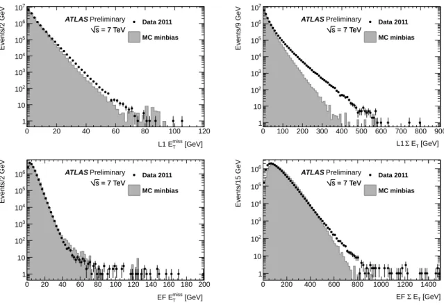
Figure 1 compares the L1 and EF E
missTand
ΣE
Tdistributions for events selected in 2011 by a random trigger during beam crossings with a simulated sample of minimum-bias events of similar
hµi. The peaksof the distributions, which account for the bulk of events, agree well with the data, but the spread in the data distributions are significantly higher, especially for
ΣE
T. There are several possible reasons for these differences. A previous ATLAS study [10] has found that PYTHIA6 does not fully describe the observed offline
ΣE
Tand E
Tmisshigh-energy tails and that these are better matched in PYTHIA8. Another source of more high E
missTand
ΣE
Tevents than expected from simulation are occasional noisy cells that give large signals. Individual bad cells can be flagged and removed at EF level, but not at L1. Events where a large number of cells give spurious energy can be detected offline, but affect the trigger distributions shown here. Finally, the measured
ΣE
Tdistributions are sensitive to the precise shape of calorimeter pulses, the details of the pileup structure, and the noise suppression scheme used.
When the luminosity increases, there are, on average, more interactions in a bunch crossing, adding more energy to the calorimeters and causing both average calorimeter energy deposit and fluctuations in energy deposit to increase; this is called “in-time” pileup. In order to meet the necessarily strict signal timing requirements while also optimizing cell energy determination, calorimeter pulses are shaped by di
fferentiation and integration, producing a quickly-rising pulse followed by a long opposite-sign tail [14]. The pulses last longer than the time between bunch crossings, so that calorimeter energy in past bunches can add positive or negative signal to energy measured in the current bunch crossing, thereby changing average cell energies and increasing measurement fluctuations; this is called “out-of-time”
pileup.
A uniform threshold of about 1 GeV was used for all trigger towers at L1 in 2011. The granularity
at which L1 energy was measured was also about 1 GeV, as is visible in some of the distributions shown
below. At EF level, in order to protect against possible spurious large negative values in individual cells,
the 2011 EF algorithm did not include in the calculation of E
missTand
ΣE
Tany cells with energy less
than 3 times the cell noise distribution width,
σcell. Rejection of all cells or towers with negative noise
fluctuations while retaining those with large positive fluctuation causes an o
ffset in the
ΣE
Tdistribution
but has negligible impact on the E
missTdistribution. This offset strongly depends on the detailed shape
[GeV]
miss
L1 ET
0 20 40 60 80 100 120
Events/2 GeV
1 10 102
103
104
105
106
107
Data 2011 MC minbias ATLAS Preliminary
= 7 TeV s = 7 TeV s
[GeV]
miss
EF ET
0 20 40 60 80 100 120 140 160 180 200
Events/2 GeV
1 10 102
103
104
105
106 Data 2011
MC minbias ATLAS Preliminary
= 7 TeV s = 7 TeV s
[GeV]
ET
Σ L1
0 100 200 300 400 500 600 700 800 900
Events/9 GeV
1 10 102
103
104
105
106
107
Data 2011 MC minbias ATLAS Preliminary
= 7 TeV s = 7 TeV s
[GeV]
ET
Σ EF
0 200 400 600 800 1000 1200 1400
Events/15 GeV
1 10 102
103
104
105
106
Data 2011 MC minbias ATLAS Preliminary
= 7 TeV s = 7 TeV s
Figure 1: L1 E
missT(top left), L1
ΣE
T(top right), EF level E
missT(bottom left) and EF level
ΣE
T(bottom right) distributions for events triggered on random colliding bunches compared with expectations from simulation.
of the noise distributions and hence also on the in-time and out-of-time pileup. The parameters used for determining calorimeter signals at L1 can in principle be tuned for the particular
µat which data is recorded, but the non pileup values were used for L1 throughout 2011. At EF level, the trigger has access to cell energies determined in Digital Signal Processors with sophisticated algorithms using pulse-shape information. In order to deal with the increasing
µ, in the middle of 2011 the constants used in shapeparameterization were changed and the
σcelldefinitions were modified to include a pileup-dependent term. Like the energy deposit due to pileup, the resulting
σcellvalues vary significantly with cell position.
For example, for
µ =8, the hadronic calorimeter
σcellranges from tens of MeV in the central part of the calorimeter, to hundreds of MeV at
|η| ∼2 to several GeV at
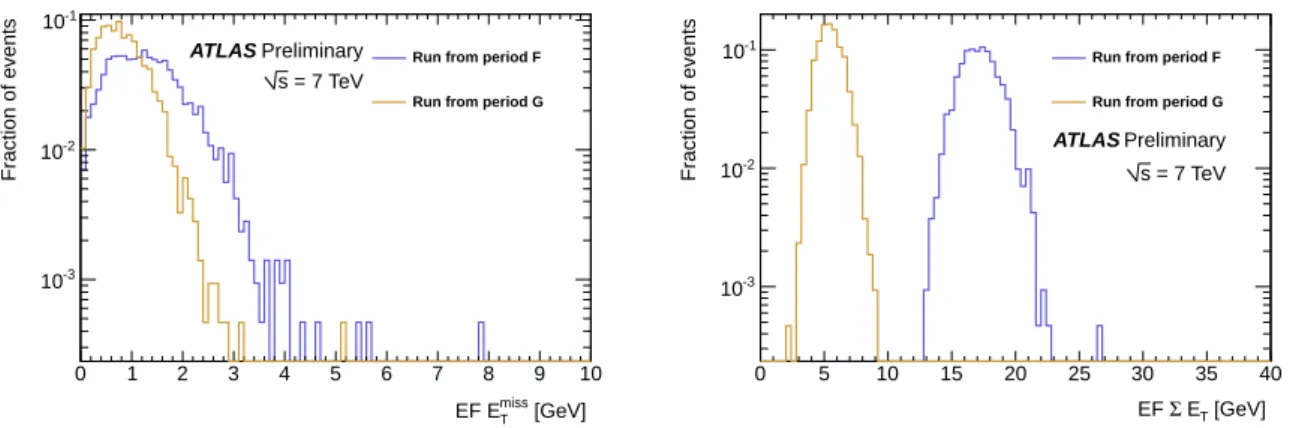
|η| ∼4. These changes in turn caused di
fferences in the measured E
missTand
ΣE
Tdistributions. Figures 2 and 3 compare the measured EF level transverse momentum distributions for empty bunch crossings and zero-bias events in data from runs in two different data-taking periods, F and G, with almost identical
hµi=7.0, before and after parameterchanges were made.
As mentioned above, calorimeter signals include effects of both in-time and out-of-time pileup. For
calorimeter signals from bunch crossings in the middle of a bunch train, the average of positive energy
signals and opposite-sign tails due to pileup roughly cancel. However, this cancellation does not occur
for the first bunches in a train, which have fewer negative-signal tails contributing and therefore have a
positive signal bias that increases as pileup becomes larger. The first bunches in a train therefore also
have a larger fraction of events with high E
missTand
ΣE
T. Figures 4 and 5 show the dependence of the
E
missTand
ΣE
Tdistributions on the bunch position in the train. The events in these figures were selected
with a random trigger on filled bunch crossings. Distributions are compared for events with the same
number of detected primary vertices, to reduce any di
fferences due to di
fferent bunches in a train having
[GeV]
miss
EF ET
0 1 2 3 4 5 6 7 8 9 10
Fraction of events
10-3
10-2
10-1
Run from period F Run from period G
ATLAS Preliminary = 7 TeV s
[GeV]
ET
Σ EF
0 5 10 15 20 25 30 35 40
Fraction of events
10-3
10-2
10-1 Run from period F
Run from period G
ATLAS Preliminary = 7 TeV s
Figure 2: EF level E
Tmiss(left) and
ΣE
T(right) distributions for empty bunch crossings compared for data recorded in two di
fferent periods. The cell signal parameterization and noise distribution width
σcellwere modified to include pileup effects in period G.
[GeV]
miss
EF ET
0 5 10 15 20 25 30 35 40
Fraction of events
10-4
10-3
10-2
Run from period F Run from period G
ATLAS Preliminary = 7 TeV s
[GeV]
ET
Σ EF
0 100 200 300 400 500 600 700 800 900 1000
Fraction of events
10-4
10-3
10-2
10-1
Run from period F Run from period G
ATLAS Preliminary = 7 TeV s
Figure 3: EF level E
Tmiss(left) and EF
ΣE
T(right) distributions for events triggered on random colliding bunches compared for data recorded in two different periods. In both cases
hµi=7.0, but the cell signalparameterization and noise distribution width
σcellwere modified to include pileup e
ffects in period G.
different instantaneous luminosities. The increase in E
Tmissand
ΣE
Tfor the first few bunches in a group are clearly visible in most of these figures. The simulation used here did not include the detailed bunch structure and its changes during the course of the 2011 data-taking period.
For the reasons discussed above, the EF level energy determination is less sensitive than that of L1 to the various e
ffects described. The tails of the simulated EF distributions are seen in Figure 1 to agree much better with the data than those of the L1 simulation.
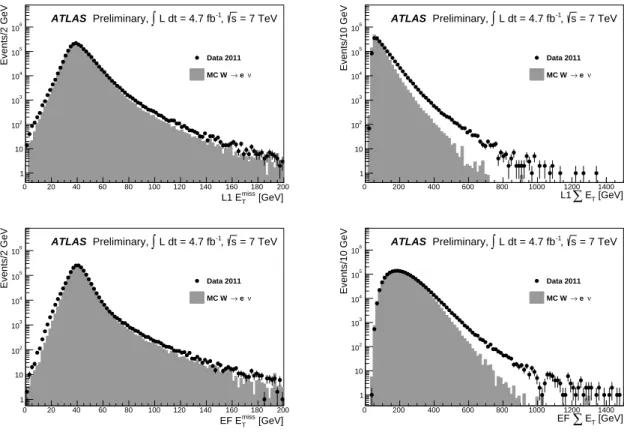
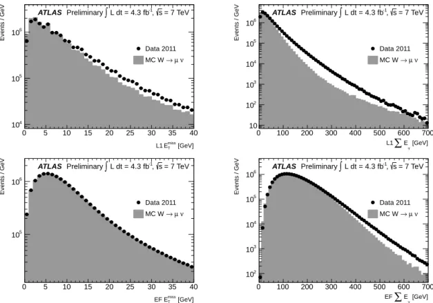
Figures 6 and 7 compare the E
missTand
ΣE
Tdistributions of data events containing candidate W’s decaying leptonically with those of the corresponding simulated event samples. The selections used to obtain these events are described in Section 2. Note that, since muons are not included in E
Tmissand
ΣE
T, the electron and muon distributions should be different. Much of the E
Tmisshere is due to neutrinos escaping the detector rather than from resolution e
ffects. Simulated E
missTdistributions agree well with the measured ones. QCD background contributes to the excess in electron-decay data events at low E
Tmiss. As is the case for zero-bias events, the data have a longer
ΣE
Ttail. The E
missTpeak at about 40 GeV for W
→eν events, as compared with the steeply falling distribution for zero-bias events shown in Figure 1, is a good illustration of the type of event feature that makes the E
missTtrigger useful for selecting events with real missing transverse momentum.
That the cause of non-zero E
missTin the bulk of events is due to fluctuations in calorimeter measure-
[GeV]
miss
L1 ET
0 20 40 60 80 100 120
Fraction of events
10-6
10-5
10-4
10-3
10-2
10-1
1
≤ 3 Bunch Xing # in train Bunch Xing # in train > 3
Preliminary ATLAS
= 7 TeV s
No. of primary vertices = 4
[GeV]
miss
EF ET
0 20 40 60 80 100 120
Fraction of events
10-6
10-5
10-4
10-3
10-2
10-1
≤ 3 Bunch Xing # in train Bunch Xing # in train > 3
Preliminary ATLAS
= 7 TeV s
No. of primary vertices = 4
[GeV]
ET
∑ L1
0 100 200 300 400 500 600 700
Fraction of events
10-6
10-5
10-4
10-3
10-2
10-1
1 Bunch Xing # in train ≤ 3
Bunch Xing # in train > 3 Preliminary ATLAS
= 7 TeV s
No. of primary vertices = 4
[GeV]
ET
EF ∑
0 100 200 300 400 500 600 700
Fraction of events
10-6
10-5
10-4
10-3
10-2
10-1
≤ 3 Bunch Xing # in train Bunch Xing # in train > 3
Preliminary ATLAS
= 7 TeV s
No. of primary vertices = 4
Figure 4: L1 (top) and EF (bottom) E
missT(left) and
ΣE
T(right) distributions for events triggered on random colliding bunches. Events are selected by requiring 4 primary vertices detected by the tracking system. Distributions are compared for events in the first 3 bunches of a train (line) and events in all other bunches (shaded).
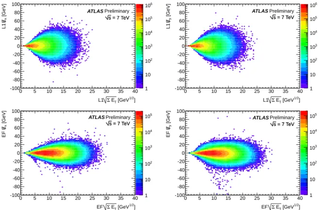
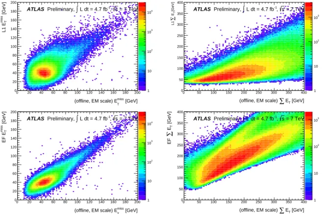
ment of transverse momentum can be seen by looking at the event-by-event correlation between E
missTand
ΣE
T. Figure 8 shows the x and
ycomponents of E
Tmissat L1 and EF plotted as a function of
√Σ
E
Tfor zero-bias events, which should have little real E
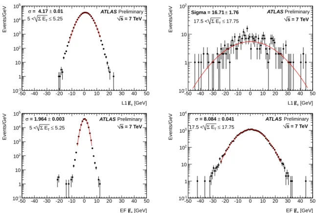
missT. As shown in Figure 9, for narrow ranges of
ΣE
Tthe central part of the E
missTdistribution is approximately Gaussian. Figure 10 shows the standard deviation of
6Exand
6Eyas a function of
√Σ
E
T. For the same
ΣE
T, the E
missTresolution at the EF level is seen to be much better than that at L1. The approximately linear dependence illustrated in these figures allows simple parameterization of the E
missTcomponent resolution as a function of
ΣE
Tby fitting it to a function of the form a
+b
√Σ
E
T, where a and b are defined so that the resolution has dimensions of energy. Although a quadratic function would better fit the L1 data, no advantage was found to doing so for trigger purposes. Note that for the ATLAS o
ffline E
Tmissanalysis [10, 11], which focused on events with particles escaping the detector, it was found sufficient to use a single constant in a parameterization of the form k
√Σ
E
T. The E
missTsignificance, XS, is then defined as the dimensionless ratio of E
missTto this resolution. Triggering on XS allows selection of events whose E
missTis unlikely to have arisen from overall calorimeter energy measurement fluctuation. As shown in Section 5 below, since it takes the fluctuations from
ΣE
Tinto account, the XS trigger rate is also much less sensitive to pileup e
ffects than the E
Tmisstriggers.
In order to prevent artificially large or small values of XS arising from small energy deposits or
[GeV]
miss
L1 ET
0 20 40 60 80 100 120
Fraction of events
10-6
10-5
10-4
10-3
10-2
10-1
≤ 3 Bunch Xing # in train Bunch Xing # in train > 3
Preliminary ATLAS
= 7 TeV s
No. of primary vertices = 10
[GeV]
miss
EF ET
0 20 40 60 80 100 120
Fraction of events
10-6
10-5
10-4
10-3
10-2
10-1
≤ 3 Bunch Xing # in train Bunch Xing # in train > 3
Preliminary ATLAS
= 7 TeV s
No. of primary vertices = 10
[GeV]
ET
∑ L1
0 100 200 300 400 500 600 700
Fraction of events
10-6
10-5
10-4
10-3
10-2
10-1
≤ 3 Bunch Xing # in train Bunch Xing # in train > 3
Preliminary ATLAS
= 7 TeV s
No. of primary vertices = 10
[GeV]
ET
EF ∑
0 100 200 300 400 500 600 700
Fraction of events
10-6
10-5
10-4
10-3
10-2
10-1 Bunch Xing # in train ≤ 3
Bunch Xing # in train > 3 Preliminary ATLAS
= 7 TeV s
No. of primary vertices = 10
Figure 5: L1 (top) and EF (bottom) E
missT(left) and
ΣE
T(right) distributions for events triggered on random colliding bunches. Events are selected by requiring 10 primary vertices detected by the tracking system. Distributions are compared for events in the first 3 bunches of a train (line) and events in all other bunches (shaded).
energy overflows it was found useful to implement several additional criteria in the XS trigger decision.
Regardless of the calculated XS value, minimum values of E
missT(typically 10 GeV) and minimum and maximum values of
ΣE
T(typically about 16 GeV and 4 TeV respectively) are imposed for an event to pass an XS trigger. At L1, events automatically pass the XS trigger if there is an overflow in the sums that give
6Exor
6Ey, and automatically fail if there is an overflow in
ΣE
T. Finally, to preserve efficiency for large E
Tmiss, an event automatically passes the XS trigger if E
Tmissis greater than some value, typically set 10 or 20 GeV higher than the lowest threshold unprescaled XE trigger. These settings, which preserve efficiency and control the rate of false triggers, result in cutoffs in some of the distributions shown in the figures below.
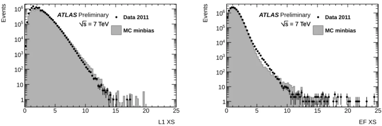
Figure 11 shows the distribution of XS at L1 and EF for events selected with a trigger firing on random bunch crossings and compares them with simulated minimum-bias events. The agreement is reasonable, with di
fferences arising from the E
missTand
ΣE
Tdi
fferences seen in Figure 1. Figure 12 compares the XS distributions for runs in two periods with di
fferent EF level characterizations of pulse shape and
σcellas described above. Some differences are visible, as would be expected from the E
missTand
ΣE
Tbehavior shown in Figure 3.
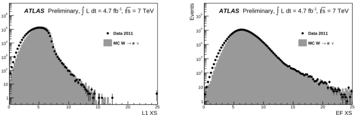
Figures 13 and 14 compare the XS distribution at L1 and EF for simulated W
→eν and W
→ µνevents with the candidate data events selected as described above. Agreement between data and
[GeV]
miss
L1 ET
0 20 40 60 80 100 120 140 160 180 200
Events/2 GeV
1 10 102
103
104
105
106
Data 2011 ν
→ e MC W
ATLAS Preliminary, ∫ L dt = 4.7 fb-1, s = 7 TeV
[GeV]
miss
EF ET
0 20 40 60 80 100 120 140 160 180 200
Events/2 GeV
1 10 102
103
104
105
106
Data 2011 ν
→ e MC W
ATLAS Preliminary, ∫ L dt = 4.7 fb-1, s = 7 TeV
[GeV]
ET
∑
L1
0 200 400 600 800 1000 1200 1400
Events/10 GeV
1 10 102
103
104
105
106
Data 2011 ν
→ e MC W
ATLAS Preliminary, ∫ L dt = 4.7 fb-1, s = 7 TeV
[GeV]
ET
∑
EF
0 200 400 600 800 1000 1200 1400
Events/10 GeV
1 10 102
103
104
105
106
Data 2011 ν
→ e MC W
ATLAS Preliminary, ∫ L dt = 4.7 fb-1, s = 7 TeV
Figure 6: Level 1 E
Tmiss(top left), L1
ΣE
T(top right), EF level E
missT(bottom left) and EF
ΣE
T(bottom right) distributions for candidate W
→eν events compared with expectations from simulation.
simulation, for these events in which E
Tmissarises from true event characteristics rather than fluctuations, is quite good, though not perfect. QCD background contributes to the excess in electron-decay data events at low XS.
The XS value is an indication of how likely it is for the E
missTin an event to arise from the imperfect measurement resolution of the total energy deposited in the calorimeter in that event. However, the approximation of a single Gaussian behavior for distributions such as those in Figure 9 is only appropriate for the central region of these plots, for which XS is low. For example, most of the transverse energy in QCD two-jet events is likely to be localized in two back-to-back regions of the calorimeter, and jet- energy resolution will give rise to large XS more frequently than the Gaussian
√Σ
E
Tmodel would predict. Therefore, XS alone cannot easily be used to separate such events from signal events containing true E
Tmiss. As a result, while triggers with low XS thresholds are useful in event selection to enhance the signal to background fraction, high-XS-threshold triggers do not provide similar advantages.
The standalone transverse-momentum triggers are those which accepted events solely based on E
Tmiss,
ΣE
T, or XS passing some threshold. The main standalone triggers used in 2011 are listed in Tables 1, 2
and 3. A large range of thresholds were used to insure that, regardless of beam luminosity, some E
missTand
ΣE
Ttriggers could always run unprescaled. As discussed in the previous paragraph, it was not useful to
set XS-trigger thresholds to high values, and these triggers almost always had to be prescaled. Except for
signatures using the L2 FEB algorithm (discussed below) the L2 and L1 algorithms were almost identical,
so typically the thresholds were set to the same value. However, because of the limited available number
of L1 firmware thresholds, L2 thresholds were sometimes varied to allow more intermediate threshold
values or to reduce rates when the highest L1 threshold was used. A number of combined triggers, which
put requirements on both transverse-momentum and other event characteristics, were also used in 2011.
[GeV]
miss
ET
L1
0 5 10 15 20 25 30 35 40
Events / GeV
104
105
106
Data 2011 ν µ
→ MC W ATLAS Preliminary ∫ L dt = 4.3 fb-1, s = 7 TeV
[GeV]
miss
ET
EF
0 5 10 15 20 25 30 35 40
Events / GeV
105
106
Data 2011 ν µ
→ MC W ATLAS Preliminary ∫ L dt = 4.3 fb-1, s = 7 TeV
[GeV]
T
∑ E L1
0 100 200 300 400 500 600 700
Events / GeV
10 102
103
104
105
106
Data 2011 ν µ
→ MC W ATLAS Preliminary ∫ L dt = 4.3 fb-1, s = 7 TeV
[GeV]
T
∑ E EF
0 100 200 300 400 500 600 700
Events / GeV
102
103
104
105
106
Data 2011 ν µ
→ MC W ATLAS Preliminary ∫ L dt = 4.3 fb-1, s = 7 TeV
Figure 7: Level 1 E
Tmiss(top left), L1
ΣE
T(top right), EF level E
missT(bottom left) and EF
ΣE
T(bottom right) distributions for candidate W
→ µνevents compared with expectations from simulation. The transverse momentum of muons is not included in these determinations of E
Tmissand
ΣE
T.
For example, a W trigger using electrons can use a lower electron transverse-momentum threshold when it is combined with an XS requirement.
Signature Thresholds [GeV] Comments
L1 L2 EF
xe20 10 10 20 Prescaled
xe30 20 20 30 Prescaled
xe40 30 30 40 Prescaled
xe50 35 35 50 Prescaled
xe60 40 40 60 Prescaled only at high luminosity xe70 50 50 70 Prescaled only at high luminosity xe70 tight 60 60 70 Not prescaled
xe80 60 60 80 Not prescaled
xe90 60 70 90 Not prescaled
Table 1: Definition of the main standalone E
missTtrigger signatures used in 2011. The su
ffix “tight” indi-
cates that the lower level thresholds were higher than the nominal ones for the same EF level threshold.
1/2] [GeV ET
Σ L1
0 5 10 15 20 25 30 35 40
[GeV]xE L1
-100 -80 -60 -40 -20 0 20 40 60 80 100
1 10 102
103
104
105
106
ATLAS Preliminary = 7 TeV s = 7 TeV s
1/2] [GeV ET
Σ EF
0 5 10 15 20 25 30 35 40
[GeV]xE EF
-100 -80 -60 -40 -20 0 20 40 60 80 100
1 10 102
103
104
105
ATLAS Preliminary = 7 TeV s = 7 TeV s
1/2] [GeV ET
Σ L1
0 5 10 15 20 25 30 35 40
[GeV]yE L1
-100 -80 -60 -40 -20 0 20 40 60 80 100
1 10 102
103
104
105
106
ATLAS Preliminary = 7 TeV s = 7 TeV s
1/2] [GeV ET
Σ EF
0 5 10 15 20 25 30 35 40
[GeV]yE EF
-100 -80 -60 -40 -20 0 20 40 60 80 100
1 10 102
103
104
105
ATLAS Preliminary = 7 TeV s = 7 TeV s
Figure 8: Level 1
6Ex(top left), L1
6Ey(top right), EF level
6Ex(bottom left) and EF
6Ey(bottom right) plotted versus the respective level
ΣE
Tfor random triggers on colliding bunches.
Signature Thresholds [GeV] Comments
L1 L2 EF
te550 180 250 550 Prescaled
300 350 550 Prescaled; settings used at high luminosity
te700 300 350 700 Not prescaled; settings in very early data collection period 300 300 700 Prescaled; settings used most of 2011
500 500 700 Prescaled; settings used at high luminosity
te900 500 500 900 Not prescaled; settings in very early data collection period 400 400 900 Prescaled; settings used most of 2011
700 700 900 Prescaled; settings used at high luminosity te1000 500 500 1000 Not prescaled; settings used most of 2011
800 800 1000 Not prescaled; settings used at high luminosity te1100 600 600 1100 Not prescaled; settings used much of 2011
500 600 1100 Not prescaled; settings used in later part of 2011 800 900 1100 Not prescaled; settings used at high luminosity te1200 700 700 1200 Not prescaled; settings used much of 2011
500 700 1200 Not prescaled; settings used in later part of 2011 800 1000 1200 Not prescaled; settings used at high luminosity
Table 2: Definition of the standalone
ΣE
Ttrigger signatures used in 2011. For each signature, Leve1 1
and Level 2 thresholds varied during 2011 as specified in the comments, but only one configuration was
active for each signature at a given time.
[GeV]
Ex
L1 -50 -40 -30 -20 -10 0 10 20 30 40 50
Events/GeV
10-1
1 10 102
103
104
105
5.25
T≤ Σ E 5 <
ATLAS Preliminary = 7 TeV s 0.01
± = 4.17 σ
[GeV]
Ex
EF -50 -40 -30 -20 -10 0 10 20 30 40 50
Events/GeV
10-1
1 10 102
103
104
105
5.25
T≤ Σ E 5 <
ATLAS Preliminary = 7 TeV s 0.003
± = 1.964 σ
[GeV]
Ex
L1 -50 -40 -30 -20 -10 0 10 20 30 40 50
Events/GeV
10-1
1 10 102
17.75
T≤ Σ E 17.5 <
ATLAS Preliminary = 7 TeV s 1.76
± Sigma = 16.71
[GeV]
Ex
EF -50 -40 -30 -20 -10 0 10 20 30 40 50
Events/GeV
10-1
1 10 102
103
104
17.75
T≤ Σ E 17.5 <
ATLAS Preliminary = 7 TeV s 0.041
± = 8.084 σ
Figure 9:
6Exdistributions for Level 1 (top) and EF level (bottom) as determined from the sum over the full set of calorimeter trigger towers (for Level 1) or calorimeter cells (for EF level) for events selected with a random trigger on colliding bunches. These are shown for two different calorimeter
ΣE
Tranges, and are compared with Gaussian fits to the distributions. The results from these fits to the peak region data points (with statistical errors as shown in the figure) are used to determine the event-by-event E
missTexpected from calorimeter energy measurement fluctuations.
Signature Thresholds Comments
L1 L2 EF
xs30 1.5 1.5 3.0 Prescaled. In later periods used L1 XE10 instead of L1 XS15.
xs45 3.0 3.0 4.5 Prescaled xs60 4.5 4.5 6.0 Prescaled xs75 5.0 5.0 7.5 Prescaled
xs100 6.0 6.0 10.0 Unprescaled at low luminosity, prescaled at high luminosity
Table 3: Definition of the standalone XS trigger signatures used in 2011.
/ ndf
χ2 3426 / 60
Offset -1.792 ± 0.005 Slope 1.169 ± 0.001
1/2] [GeV ET
Σ L1
0 5 10 15 20 25
[GeV]xσ L1
0 5 10 15 20 25 30 35
/ ndf
χ2 3426 / 60
Offset -1.792 ± 0.005 Slope 1.169 ± 0.001 ATLAS Preliminary
= 7 TeV s = 7 TeV s = 7 TeV s
/ ndf
χ2 207.3 / 81
Offset -0.5493 ± 0.0022 Slope 0.4918 ± 0.0003
1/2] [GeV ET
Σ EF
0 5 10 15 20 25
[Gev]xσ EF
0 5 10 15 20 25 30 35
/ ndf
χ2 207.3 / 81
Offset -0.5493 ± 0.0022 Slope 0.4918 ± 0.0003
ATLAS Preliminary = 7 TeV s = 7 TeV s = 7 TeV s
/ ndf
χ2 3081 / 60
Offset -1.787 ± 0.005 Slope 1.156 ± 0.001
1/2] [GeV ET
Σ L1
0 5 10 15 20 25
[GeV]yσ L1
0 5 10 15 20 25 30 35
/ ndf
χ2 3081 / 60
Offset -1.787 ± 0.005 Slope 1.156 ± 0.001 ATLAS Preliminary
= 7 TeV s = 7 TeV s = 7 TeV s
/ ndf
χ2 371.6 / 81
Offset -0.6035 ± 0.0022 Slope 0.5044 ± 0.0003
1/2] [GeV ET
Σ EF
0 5 10 15 20 25
[Gev]yσ EF
0 5 10 15 20 25 30 35
/ ndf
χ2 371.6 / 81
Offset -0.6035 ± 0.0022 Slope 0.5044 ± 0.0003
ATLAS Preliminary = 7 TeV s = 7 TeV s = 7 TeV s
Figure 10: Standard deviation of
6Ex(left) and
6Ey(right) for L1 (top) and EF (right) as determined from the sum over the full set of calorimeter trigger towers (for Level 1) or calorimeter cells (for EF level) for events selected with a random trigger on colliding bunches. A linear fit to the standard deviation as a function of the square root of the total calorimeter
ΣE
Tis used to determine the event-by-event E
missTexpected from calorimeter energy measurement fluctuations. The error bars are the statistical errors on the standard deviation determined from a Gaussian fit to the individual
6Exand
6Eydistributions for each
ΣE
Tbin. The non-linearity at Level 1 means that fewer events than predicted by the line will fluctuate above any given
6Exor
6Eyvalue.
L1 XS
0 5 10 15 20 25
Events
1 10 102
103
104
105
106
Data 2011 MC minbias ATLAS Preliminary
= 7 TeV s = 7 TeV s
EF XS
0 5 10 15 20 25
Events
1 10 102
103
104
105
106
Data 2011 MC minbias ATLAS Preliminary
= 7 TeV s = 7 TeV s