ATLAS NOTE ATLAS-CONF-2013-082

A TLAS-CONF-2013-082 09 August 2013

ATLAS NOTE

ATLAS-CONF-2013-082

August 8, 2013

Performance of Missing Transverse Momentum Reconstruction in ATLAS studied in Proton-Proton Collisions recorded in 2012 at √

s = 8 TeV

ATLAS Collaboration

Abstract

The performance of the missing transverse momentum reconstruction in the ATLAS detector is evaluated using data collected in 2012 in proton-proton collisions at a centre-of- mass energy of 8 TeV. An optimised reconstruction and calibration of the missing trans- verse momentum is used and the effects arising from additional proton-proton interactions superimposed on the hard physics process are suppressed with various methods. Results are shown for a data sample corresponding to an integrated luminosity of about 20 fb

and for events with different topologies with or without genuine missing transverse momentum due to undetected particles. Estimates of the systematic uncertainty on the missing transverse momentum measurement are also presented.

© Copyright 2013 CERN for the benefit of the ATLAS Collaboration.

Reproduction of this article or parts of it is allowed as specified in the CC-BY-3.0 license.

1 Introduction

In a hadron collider event the missing transverse momentum is defined as the momentum imbalance in the plane transverse to the beam axis, where momentum conservation is useful. Such an imbalance may signal the presence of undetectable particles, such as neutrinos or new weakly-interacting particles. The vector momentum imbalance in the transverse plane is obtained from the negative vector sum of the momenta of all particles detected in a proton-proton ( pp) collision and is denoted as missing transverse momentum, E

. The symbol E

is used for its magnitude.

An optimised reconstruction and calibration of E

[1] was developed by the ATLAS Collabora- tion. The E

measurement is significantly affected by the contributions of additional pp collisions superimposed on the hard physics process, referred to as pile-up in the following, so methods were de- veloped to suppress such contributions [2]. This note describes the performance, in terms of resolution, response and tails, of the reconstructed E

after pile-up suppression.

The event samples used to assess the quality of the E

reconstruction are minimum bias events, events with leptonically decaying W and Z bosons and simulated events with large jet multiplicity and/or large missing transverse momentum, such as H → ττ, t¯ t and simulated supersymmetric (SUSY) events.

These test the detector capability in the reconstruction and calibration of different physics objects, the optimization of the E

calculation and the methods of pile-up suppression. The E

performance is studied in both data and Monte Carlo simulation and comparisons are made. The study of E

perfor- mance in events where genuine E

is present allows for a validation of the E

scale. In simulated events, the genuine E

is calculated from all non-interacting particles in the event, including neutrinos from heavy flavour decay, and is referred to as true E

(E

) in the following.

An important requirement on the measurement of E

is maximizing detector coverage and reduc- ing the effect of finite detector resolution, the presence of dead regions and different sources of noise, as well as cosmic-ray and beam-halo muons crossing the detector, that can produce fake E

. The ATLAS calorimeter coverage extends to large pseudorapidities

to reduce the impact of high energy particles es- caping in the very forward direction. However, there are transition regions between different calorimeters containing inactive material which lead to increased fake E

. Selection criteria are applied to reduce the impact of these sources of fake E

.

This note is organised as follows. Section 2 gives a brief introduction to the ATLAS detector. Sec- tions 3 and 4 describe the data and Monte Carlo samples used and the event selections applied. Section 5 outlines how E

is reconstructed and calibrated and Section 6 summarizes the methods used to miti- gate the pile-up effects. Section 7 presents the E

performance for data and Monte Carlo simulation in events from different physics channels with various topologies. Finally, the systematic uncertainty on the E

absolute scale is discussed in Section 8.

2 The ATLAS Detector

The ATLAS detector [3] is a multipurpose particle physics apparatus with a forward-backward symmet- ric cylindrical geometry and near 4π coverage in solid angle. The inner tracking detector (ID) covers the pseudorapidity range |η| < 2.5, and consists of a silicon pixel detector, a silicon microstrip detector (SCT), and, for |η| < 2.0, a transition radiation tracker (TRT). The ID is surrounded by a thin supercon- ducting solenoid providing a 2 T magnetic field. A high-granularity lead/liquid-argon (LAr) sampling electromagnetic calorimeter covers the region |η| < 3.2. A steel/scintillator-tile calorimeter provides

1

ATLAS uses a right-handed coordinate system with its origin at the nominal interaction point (IP) in the centre of the

detector and the z-axis coinciding with the axis of the beam pipe. The x-axis points from the IP to the centre of the LHC ring,

and the y axis points upward. Cylindrical coordinates (r, φ) are used in the transverse plane, φ being the azimuthal angle around

the beam pipe. The pseudorapidity is defined in terms of the polar angle θ as η = − ln tan(θ/2).

hadronic coverage in the range |η| < 1.7. LAr technology is also used for the hadronic calorimeters in the end-cap region 1.5 < |η| < 3.2 and for both electromagnetic and hadronic measurements in the forward region up to |η| < 4.9. The muon spectrometer surrounds the calorimeters. It consists of three large air-core superconducting toroid systems, precision tracking chambers providing accurate muon tracking out to |η| = 2.7, and additional detectors for triggering in the region |η| < 2.4.

3 Data samples and event selection

During 2012, proton-proton ( pp) collisions at a centre-of-mass energy of 8 TeV were recorded with stable proton beams and nominal ATLAS magnetic field conditions. Only data with a fully functioning calorimeter, inner detector and muon spectrometer are analysed.

Selection criteria [4] are applied which reduce the impact of instrumental noise and out-of-time energy deposits in the calorimeter from cosmic-rays or beam-induced background, suppressing the effect of fake E

from those sources.

The data sets used correspond to a total integrated luminosity [5, 6] of approximately 20 fb

, col- lected in 2012 with a bunch crossing interval (bunch spacing) of 50 ns. The mean number of interactions per bunch crossing (hµi)

was about 20.7, with hµi reaching values up to 35 at the beginning of a fill during the 2012 LHC running period.

Trigger and selection criteria applied for the study of minimum bias events and events with leptoni- cally decaying W and Z bosons are described in the following.

3.1 Minimum bias events

Minimum bias events were selected both by a random trigger and by the minimum bias trigger scintil- lators (MBTS), which are mounted at each end of the detector in front of the LAr end-cap calorimeter cryostats [7]. For each event, at least one good primary vertex is required with a z displacement from the nominal pp interaction point of less than 200 mm and with at least five associated tracks.

3.2 Z → `` event selection

Candidate Z → `` events, where ` is an electron or a muon, are required to pass an electron, photon or muon trigger with a transverse momentum, p

, threshold between 15 and 20 GeV, where the exact trigger selection varies depending on the data period analysed. For each event, at least one good primary vertex is required with a z displacement from the nominal pp interaction point of less than 200 mm and with at least three associated tracks.

The selection of Z → µµ events requires the presence of exactly two good muons. A good muon is defined to be a muon reconstructed in the muon spectrometer with a matched track in the inner detector with transverse momentum above 25 GeV and |η| < 2.5 [8]. Additional requirements on the number of hits used to reconstruct the tracks in the inner detector are applied. The z displacement of the muon tracks from the primary vertex is required to be less than 10 mm. Isolation criteria are applied around the muon track.

The selection of Z → ee events requires the presence of exactly two identified electrons with |η| <

2.47, which pass the “medium” identification criteria [9, 10], optimized for 2012 data, and have trans- verse momenta above 25 GeV. Electron candidates in the electromagnetic calorimeter transition region, 1.37 < |η| < 1.52, are not considered for this study.

2

The mean number of inelastic proton proton interactions per bunch is averaged over one luminosity block lasting typically

60 seconds and calculated from the measured instantaneous luminosity, L, the inelastic cross section, σ

, and the average

number of colliding bunch pairs per revolution in the LHC, N

× f

: hµi= L × σ

/(N

× f

)

In both the Z → ee and the Z → µµ selections, the two leptons are required to have opposite charge and the reconstructed invariant mass of the di-lepton system, m

, is required to be consistent with the Z mass, 66 < m

< 116 GeV.

3.3 W → `ν event selection

Lepton candidates are selected with lepton identification criteria similar to those used for the Z selection.

An isolation cut is applied around the electron energy deposits in the calorimeter to reduce contamination from jets. The event is required to contain exactly one reconstructed lepton (electron or muon). The E

, calculated as described in Section 5, is required to be greater than 25 GeV. The reconstructed mass of the transverse momentum of the lepton, p

, and E

, m

= q

2p

E

(1 − cos φ), where φ is the azimuthal angle between the lepton momentum and E

directions, must satisfy m

> 50 GeV.

4 Monte Carlo simulation samples

Monte Carlo (MC) samples of Z → `` and W → `ν production are generated with the next-to-leading (NLO) order P OWHEG [11] model, with the final state partons showered by the P YTHIA 8 program [12, 13], using the CT10 next-to-leading order (NLO) parton distribution function (PDF) [14] and the ATLAS AU2 tune [15]. Samples of Z → `` generated with A LPGEN [16] are also used for some additional data- MC comparison. The t¯ t events are generated with the MC@NLO program [17]. The Z → ττ and H → ττ events with m

= 125 GeV, from direct production or produced through the Vector Boson Fusion mechanism (VBF H → ττ), are also generated with P OWHEG . The performance has also been tested with samples of simulated supersymmetry (SUSY) events. An R-parity conserving simplified model is used, in which pair-production of gluinos is simulated. The gluinos are assumed to decay with unit probability to a top quark, and anti-top quark and a stable invisible neutralino with mass of 1 GeV. Two different values of the gluino mass are used, 0.5 TeV (labelled SUSY500 in what follows) and 1.0 TeV (SUSY1000). These samples were generated using HERWIG++ [18].

Additional inelastic pp interactions, known as pile-up interactions, are generated using the P YHIA 8 program with the ATLAS MC12 A2M tune [15] and the MSTW08 leading order (LO) PDF [19]. The proton-proton bunches are organised in trains, with 50 ns spacing between bunches, closely matching the bunch structure of the LHC. Therefore the simulation contains effects from pile-up arising from bunches before or after the bunch crossing in which the event of interest was triggered (out-of-time pile-up). The MC simulation samples are weighted such that the distribution of the average number of interactions per bunch crossing matches that observed in the 2012 data sample, to ensure that the pile-up interactions are accurately described. When the pile-up conditions are not specified for a given figure, they should be assumed to be matched to those observed in the 2012 data sample used.

The G EANT 4 software toolkit [20] within the ATLAS simulation framework [21] simulates the prop- agation of the generated particles through the ATLAS detector and their interactions with the detector material. It was used for all samples.

The same trigger and event selection criteria used for Z → `` and W → `ν data are also applied to

the simulated Z → `` and W → `ν events. The t¯ t events are required to contain at least one electron or

muon with p

> 25 GeV. For Z → ττ and H → ττ simulations the lepton-hadron events are selected,

where one τ decays to a lepton (electron or muon) and the other to hadrons, requiring an electron or a

muon and an identified τ-jet , both with p

> 20 GeV.

5 E ^miss

T reconstruction and calibration

The E

reconstruction [1] uses energy deposits in the calorimeters and muons reconstructed in the muon spectrometer. Also muons formed by segments which are matched to inner detector tracks ex- trapolated to the muon spectrometer (tagged muons) are used to recover muons, typically of low pT, which did not cross enough precision muon chambers to allow an independent momentum measurement in the muon spectrometer. Tracks are added to recover the contribution from low-p

particles which are missed in the calorimeters.

The E

calculation uses reconstructed and calibrated physics objects. Calorimeter energy deposits are associated with a reconstructed and identified high-p

parent object in a specific order: electrons, photons, hadronically decaying τ-leptons, jets and finally muons. Deposits not associated with any such objects are also taken into account in the E

calculation. The E

is calculated as follows:

E

= E

+ E

+ E

+ E

+ E

x(y)

+ E

, (1)

where each term is calculated as the negative sum of the calibrated reconstructed objects, projected onto the x and y directions. Because of the high granularity of the calorimeter, it is important to suppress noise contributions and to use in the E

calculation, in addition to the high-p

reconstructed objects, only the calorimeter energy deposits containing a significant signal. This is achieved by calculating the E

soft term using only energy deposits from topological clusters, referred to as topoclusters hereafter [22]. To avoid double counting energy, the parametrized muon energy loss in the calorimeters is subtracted in the E

calculation if the combined muon momentum is used [1].

In Equation 1, electrons are calibrated with the standard ATLAS electron calibration [10] and photons are calibrated at the electromagnetic scale (EM)

. The τ-jets are calibrated with the local cluster weight- ing (LCW) [23, 24] which involves classifying the energy depositions as electromagnetic or hadronic, and weighting them appropriately when computing the topocluster energy, an offset is subtracted to suppress the pile-up effects, and the tau energy scale (TES) correction [25] is applied. The jets are re- constructed with the anti-k

algorithm [26], with distance parameter R = 0.4. Each jet is corrected for the pile-up and is subsequently calibrated with the LCW+JES scheme, where JES is the jet energy scale [24]. Only jets with calibrated p

greater than 20 GeV are used to calculate the jet term in Equation 1.

The soft term

is calculated from topoclusters and tracks not associated to high-p

objects (i.e. from unassociated topoclusters and tracks), the topoclusters being calibrated using the LCW technique and removing any overlap between tracks and topoclusters.

The E

is sometimes described by its azimuthal angle and magnitude, φ

and E

. The total transverse energy in the calorimeters, P

E

, which includes also the unassociated low- p

tracks used in the soft term, is an important quantity to parameterise and understand the E

per- formance. It is defined as the scalar sum:

X E

= X

E

+ X

E

+ X

E

+ X

E

+ X

E

, (2)

which is the scalar sum of the transverse energy of reconstructed and calibrated objects and of the soft term according to the scheme described above for E

. The total transverse energy in the event is

3

The EM scale is the basic calorimeter signal scale for the ATLAS calorimeters. It provides the correct scale for energy deposited by electromagnetic showers. It does not correct for the lower energy hadron shower response nor for energy losses in the dead material.

4

It should be noted that the E

T

in Equation 1 includes contributions both from jets with p

< 20 GeV and from unassociated topoclusters/tracks. Previously [1, 2] those contributions were calculated separately, and were denoted as

E

and E

respectively.

obtained by summing the p

of muons and the P

E

in the calorimeters:

X

E

(event) = X

E

+ X

p

. (3)

6 Methods for pile-up suppression in E ^miss

T

In Ref. [2], it was shown that a clear deterioration of the performance is observed when the average number of pile-up interactions per event increases. In the same note it was shown that the pile-up af- fects also the E

response. Methods to suppress pile-up are therefore needed which can restore the E

resolution to values more similar to the ones observed in the absence of pile-up, without spoiling the E

response and without creating fake E

.

All E

terms in Equations 1 and 2 are affected by pile-up, but the terms which are most affected are the jets and soft term, because the pile-up largely produces hadronic energy and they are recon- structed from larger regions in the calorimeters. Methods for the suppression of pile-up in these terms are summarized in this section.

6.1 Pile-up suppression in the E

T

jet term based on tracks

Pile-up not only distorts the energy reconstructed in jets but can also create additional jets. As discussed in Section 5, the jets with p

> 20 GeV used in the E

reconstruction are already corrected for pile-up effects, using the jet area method [27]. The corrected jet p

is calculated as p

− ρ × A

, where ρ is the transverse momentum density in the event, calculated as the median of p

/A

from the jets built with the recursive recombination algorithm k

[28, 29] with distance parameter R = 0.4 in |η| < 2 and A

is the area of the jet. This correction captures event-by-event fluctuations and has no dependence on pile-up modeling.

To further suppress the jets originating from pile-up, a cut is applied based on the jet vertex fraction, JVF [30], i.e. the fraction of momenta of tracks matched to the jet which are associated with the hard scattering vertex. JVF is defined as:

JVF = X

tracksjet,PV

p

/ X

tracksjet

p

, (4)

where the sums are taken over the tracks matched to the jet and PV denotes the tracks associated to the primary vertex

. Only tracks with p

> 400 MeV and passing further quality criteria relating to impact parameters and number of hits in different ID sub-detectors are used to make primary vertices.

Jets with no associated tracks are assigned JVF = − 1. Within this note, any jet with p

< 50 GeV and with |η| < 2.4 which does not satisfy |JVF| > 0 is discarded in the calculation of the pile-up suppressed E

. This requirement, which discards only those jets, inside the tracker acceptance |η| < 2.4, which have no tracks originating from the leading primary vertex, reduces the jets originating from pile-up. Jets with no associated tracks, which have JVF = −1 and include all jets outside the inner detector region, are kept.

6.2 Pile-up suppression in the E

T

soft term based on tracks The pile-up largely affects the soft term. Since the E

T

can have an important contribution to the momentum balance in the event, completely neglecting its contribution in the E

reconstruction

5

Defined as the primary vertex that has maximal P

p

of the tracks associated with it.

gives a poorer performance [2]. Two different methods for suppressing the pile-up in the soft term are described in the following, one based on the use of tracks and the other one based on the jet area method.

Tracks provide an excellent method for pile-up suppression, since they can be associated with the pri- mary vertex from the hard scattering collision. Pile-up suppression is achieved by scaling the E

T

with the soft term vertex fraction (STVF) i.e. the fraction of momenta of tracks matched to the soft term which are associated with the hard scattering vertex. It is calculated, in a similar way as JVF, as:

STVF = X

tracksSoftTerm,PV

p

/ X

tracksSoftTerm

p

, (5)

where the sums are taken over the tracks unmatched to physics objects and PV denotes the tracks asso- ciated to the primary vertex.

The E

T

is multiplied by the STVF factor and the E

calculated with this corrected soft term is named STVF.

6.3 Pile-up suppression in the E

T

soft term using the jet area method This method for the pile-up subtraction in the E

T

is based on the jet area, which is also the correction used for jets described in Section 6.1. The essential ingredients are:

• the reclustering of the energy from topoclusters and tracks entering in the E

T

. For this

task, jets are reconstructed down to p

= 0 using the k

algorithm

• the event transverse momentum density ρ is used to determine the contribution due to pile-up in the jet area, which is subtracted from each k

jet: p

= p

− ρ × A

. The p

= 0 if p

< ρ × A

• finally a track-based filter is applied to k

jets, similar to the one used for jets, and the E

T

is

calculated using only the k

jets after pile-up subtraction which satisfy |JVF| > 0.25.

Two different E

T

calculations are considered in this note and the E

is then recalculated using each of them. The two methods differ only in their calculation of the ρ, as follows:

• the ρ is calculated as the median of p

/A

from the k

jets (R = 0.4) reconstructed from topoclus- ters and tracks associated to the soft term in |η| < 1.8 (plateau region) and extrapolated to the forward region using the ρ shape as a function of η, determined from minimum bias events in the 2012 data. The distribution of ρ(η) is fitted with an analytic function, obtained by summing two gaussians, one for the plateau region (depending on the P

E

of the event) and the other for the forward region (whose parameters depend on hµi of the events). The soft term jets are formed using the k

algorithm with R = 0.6 and they are corrected and filtered as explained above. The corresponding E

is named Extrapolated Jet Area Filtered.

• the ρ is calculated as the median of p

/A

from the k

jets (R = 0.8) reconstructed from topoclus- ters and tracks associated to the soft term in |η| < 5. The soft term jets are formed using the k

algorithm with R = 0.4 and they are corrected and filtered as explained above. The corresponding E

is named Jet Area Filtered.

6.4 Definitions

In the following sections, the performances of the E

reconstruction before and after the pile-up

suppression are shown for the different methods based on tracks or using jet area, in terms of resolution,

response and tails for data and MC events. Four E

calculations are compared, one without a special pile-up suppression treatment and three with pile-up mitigation techniques applied. They differ only in the soft term and the jet term.

• the E

before pile-up suppression has the jet term calculated from all jets with p

> 20 GeV corrected with jet area and the soft term calculated from unassociated topoclusters and tracks, as described in Section 5.

• the three pile-up suppressed variants have the same jet term formed from all jets (corrected with jet area) with p

> 50 GeV and from the ones with 20 < p

< 50 GeV and |η|< 2.4 with |JVF| > 0.

They differ in the soft term as described in this section; one uses the track based STVF weight (E

STVF) and the two others use the jet area pile-up suppression (E

Extrapolated Jet Area Filtered and Jet Area Filtered).

7 Study of E ^miss

T performance in different event topologies

7.1 Characterization of samples used for the study of E

T

performance

The E

performance depends on the event topology, i.e. presence of genuine E

, presence of leptons, jet activity, etc. The values of quantities relevant for E

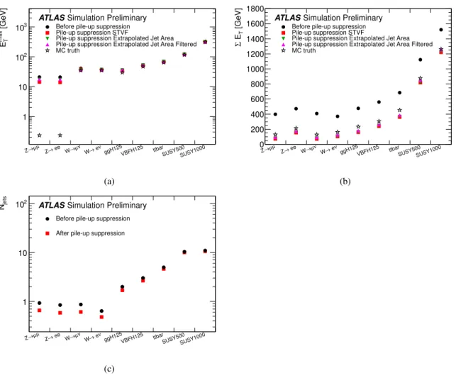
studies in the MC samples used in this note are shown in Figure 1 and Figure 2. In Figure 1 the reconstructed E

and P

E

before and after pile-up suppression are compared with the true values. As can be seen, the P

E

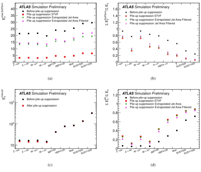
is strongly suppressed by all the pile-up suppression methods and it is closer to the true value. The average number of jets before and after the pile-up suppression (JVF cut) is also shown. Figure 2 shows the importance of the soft term and of the jet term in the different samples. The average value of E

T

is not much

different in the various samples but its contribution is dominant in Z samples and important in W events, while it becomes less important in events with higher jet multiplicity, where the E

is dominant, as can be seen from the distribution of the ratios of P

E

/ P

E

and P E

/ P

E

. 7.2 Comparison of E

T

distributions in data and MC simulation

In this section some basic distributions in Z → `` and W → `ν events from data are compared with the expected distributions from the MC samples, before and after pile-up suppression. The comparison is done also separately for each of the various terms in Equations 1 and 2.

7.2.1 E

T

distributions in Z → `` events

The Z → `` channel is well-suited to the study of E

performance because of its clean event signature and the relatively large cross-section. In general, apart from a small contribution from the semi-leptonic decay of heavy-flavour hadrons in jets or background contributions, no genuine E

is expected in these events. Thus most of the E

reconstructed in these events is a direct result of imperfections in the reconstruction process or in the detector response.

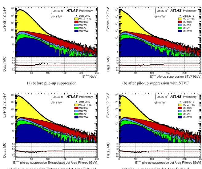
The distributions of E

for data are shown in Figure 3 for Z → µµ events. The MC simulation

expectations, from Z → µµ events and from the dominant backgrounds, are superimposed. Each MC

sample is weighted with its corresponding cross-section and then the total MC expectation is normalized

to the number of events in data. A good agreement between data and MC simulation is observed in

the E

distribution, both before and after pile-up suppression. The tails in the E

distribution in

Z → `` data are compatible with either signal candidates or with backgrounds, including t¯ t and di-boson

events, all involving real E

, demonstrating that the instrumental effects are well described.

µµ

Z→ ee

Z→ W→µν eν

W→ ggH125VBFH125 ttbar

SUSY500SUSY1000

[GeV]miss TE

1 10 102

103 Before pile-up suppression Pile-up suppression STVF

Pile-up suppression Extrapolated Jet Area Pile-up suppression Extrapolated Jet Area Filtered MC truth

ATLASSimulation Preliminary

(a)

µµ

Z→ Z→ ee W→µνW→ eνggH125VBFH125 ttbar

SUSY500SUSY1000

[GeV]T EΣ

0 200 400 600 800 1000 1200 1400 1600 1800

Before pile-up suppression Pile-up suppression STVF

Pile-up suppression Extrapolated Jet Area Pile-up suppression Extrapolated Jet Area Filtered MC truth

ATLASSimulation Preliminary

(b)

µµ

Z→ Z→ ee W→µν W→ eνggH125VBFH125 ttbar

SUSY500SUSY1000

jetsN

1 10 102

Before pile-up suppression After pile-up suppression

ATLASSimulation Preliminary

(c)

Figure 1: Average values of E

(a), P

E

(b) and of the number of jets with p

> 20 GeV (c) in the

MC samples used. The values before pile-up suppression and the values after pile-up suppression with

different methods are shown. The true MC values are also shown in (a) and (b).

µµ

Z→ Z→ ee W→µν W→ eνggH125VBFH125 ttbar

SUSY500SUSY1000 miss,SoftTerm TE

0 5 10 15 20 25 30 35

40 Before pile-up suppression Pile-up suppression STVF

Pile-up suppression Extrapolated Jet Area Pile-up suppression Extrapolated Jet Area Filtered

ATLASSimulation Preliminary

(a)

µµ

Z→ Z→ ee W→µνW→ eν H→ττ →ττ VBFH

tt

SUSY500SUSY1000 T EΣ/SoftTerm T EΣ

0 0.2 0.4 0.6 0.8 1 1.2 1.4 1.6

Before pile-up suppression Pile-up suppression STVF

Pile-up suppression Extrapolated Jet Area Filtered Pile-up suppression Jet Area Filtered

ATLASSimulation Preliminary

(b)

µµ

Z→ ee

Z→ W→µν eν

W→ ggH125VBFH125 ttbar

SUSY500SUSY1000 miss,jet TE

10 102

103

Before pile-up suppression After pile-up suppression

ATLASSimulation Preliminary

(c)

µµ

Z→ Z→ ee W→µνW→ eνggH125VBFH125 ttbar

SUSY500SUSY1000 T EΣ/jet T EΣ

0 0.2 0.4 0.6 0.8 1

1.2 Before pile-up suppression Pile-up suppression STVF

Pile-up suppression Extrapolated Jet Area Pile-up suppression Extrapolated Jet Area Filtered

ATLASSimulation Preliminary

(d)

Figure 2: E

T

(a), ratio of P

E

over P

E

(b), E

(c) and ratio of P

E

over

P E

(d) in the samples used. The values before pile-up suppression and after pile-up suppression are

shown.

The contributions to E

from jets before and after applying the JVF cut and from reconstructed muons are shown separately in Figure 4. The peak at zero in the distribution of the jet term corresponds to events where there are no jets with p

above 20 GeV, and the small values (< 20 GeV) in the distribution are due to events with two or more jets whose transverse momenta partially balance. The agreement for the jet term is within 20% both before and after pile-up suppression. After pile-up suppression, some more disagreement is observed in the region below 20 GeV populated by events with two or more jets.

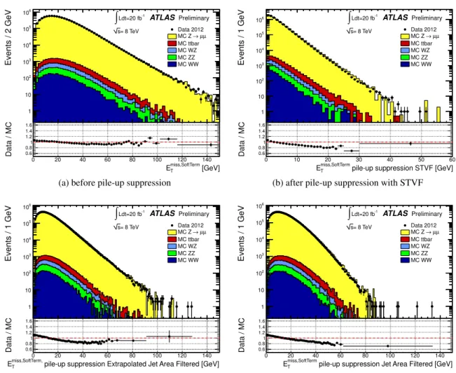
This is probably due to the poor modeling of the number of additional jets in the MC simulation. The contributions to E

from the E

T

before and after pile-up suppression are shown in Figure 5.

The data-MC agreement for the E

T

is slightly worse after pile-up suppression, due to some discrepancy observed in the STVF fraction, which suffers from the mis-modeling of the track activity in MC simulation.

0 50 100 150 200 250

Events / 2 GeV

1 10 102

103

104

105

106

Data 2012 µ µ MC Z → MC ttbar MC WZ MC ZZ MC WW Ldt=20 fb-1

∫

= 8 TeV s

ATLASPreliminary

[GeV]

miss

ET

0 50 100 150 200 250

Data / MC ^0.6

0.81 1.2 1.4 1.6

(a) before pile-up suppression

0 50 100 150 200 250

Events / 2 GeV

1 10 102

103

104

105

106

Data 2012 µ µ MC Z → MC ttbar MC WZ MC ZZ MC WW Ldt=20 fb-1

∫

= 8 TeV s

ATLAS Preliminary

pile-up suppression STVF [GeV]

miss

ET

0 50 100 150 200 250

Data / MC ^0.6

0.81 1.2 1.4 1.6

(b) after pile-up suppression with STVF

0 50 100 150 200 250

Events / 2 GeV

1 10 102

103

104

105

106

Data 2012 µ µ

→ MC Z MC ttbar MC WZ MC ZZ MC WW Ldt=20 fb-1

∫

= 8 TeV s

ATLASPreliminary

pile-up suppression Extrapolated Jet Area Filtered [GeV]

miss

ET

0 50 100 150 200 250

Data / MC ^0.6

0.81 1.2 1.4 1.6

(c) pile-up suppression Extrapolated Jet Area Filtered

0 50 100 150 200 250

Events / 2 GeV

1 10 102

103

104

105

106

Data 2012 µ µ

→ MC Z MC ttbar MC WZ MC ZZ MC WW Ldt=20 fb-1

∫

= 8 TeV s

ATLAS Preliminary

pile-up suppression Jet Area Filtered [GeV]

miss

ET

0 50 100 150 200 250

Data / MC ^0.6

0.81 1.2 1.4 1.6

(d) pile-up suppression Jet Area Filtered

Figure 3: Distribution of E

(a) as measured in a data sample of Z → µµ events before pile-up sup-

pression. Distributions of E

after pile-up suppression with the STVF (b), with the Extrapolated Jet

Area Filtered (c) and with the Jet Area Filtered (d) methods. The expectation from Monte Carlo simula-

tion is superimposed and normalized to data, after each MC sample is weighted with its corresponding

cross-section. The lower parts of the figures show the ratio of data over MC.

0 50 100 150 200 250 300 350

Events / 2 GeV

1 10 102

103

104

105

106

107

Data 2012 µ µ MC Z → MC ttbar MC WZ MC ZZ MC WW Ldt=20 fb-1

∫

= 8 TeV s

ATLASPreliminary

[GeV]

miss,jets

ET

0 50 100 150 200 250 300 350

Data / MC ^0.60.8

1 1.2 1.4 1.6

(a) before pile-up suppression

0 50 100 150 200 250 300 350

Events / 2 GeV

1 10 102

103

104

105

106

107

Data 2012 µ µ MC Z → MC ttbar MC WZ MC ZZ MC WW Ldt=20 fb-1

∫

= 8 TeV s

ATLAS Preliminary

after pile-up suppression [GeV]

miss,jets

ET

0 50 100 150 200 250 300 350

Data / MC ^0.60.8

1 1.2 1.4 1.6

(b) after pile-up suppression with JVF

0 50 100 150 200 250 300 350

Events / 2 GeV

1 10 102

103

104

105

106

Data 2012 µ µ

→ MC Z MC ttbar MC WZ MC ZZ MC WW Ldt=20 fb-1

∫

= 8 TeV s

ATLASPreliminary

[GeV]

miss,µ

ET

0 50 100 150 200 250 300 350

Data / MC ^0.6

0.81 1.2 1.4 1.6

(c) before pile-up suppression

Figure 4: Distribution of E

computed from reconstructed jets with p

> 20 GeV (E

) (a), after

pile-up suppression with JVF (b) for Z → µµ data. The contribution from the muons (E

) is shown

separately in (c). The expectation from Monte Carlo simulation is superimposed and normalized to data,

after each MC sample is weighted with its corresponding cross-section. The lower parts of the figures

show the ratio of data over MC.

0 20 40 60 80 100 120 140

Events / 2 GeV

1 10 102

103

104

105

106

Data 2012 µ µ

→ MC Z MC ttbar MC WZ MC ZZ MC WW Ldt=20 fb-1

∫

= 8 TeV s

ATLASPreliminary

[GeV]

miss,SoftTerm

ET

0 20 40 60 80 100 120 140

Data / MC ^0.6

0.81 1.2 1.4 1.6

(a) before pile-up suppression

0 10 20 30 40 50 60

Events / 1 GeV

1 10 102

103

104

105

106

Data 2012 µ µ

→ MC Z MC ttbar MC WZ MC ZZ MC WW Ldt=20 fb-1

∫

= 8 TeV s

ATLAS Preliminary

pile-up suppression STVF [GeV]

miss,SoftTerm

ET

0 10 20 30 40 50 60

Data / MC ^0.6

0.81 1.2 1.4 1.6

(b) after pile-up suppression with STVF

0 20 40 60 80 100 120 140

Events / 1 GeV

1 10 102

103

104

105

106

Data 2012 µ µ

→ MC Z MC ttbar MC WZ MC ZZ MC WW Ldt=20 fb-1

∫

= 8 TeV s

ATLASPreliminary

pile-up suppression Extrapolated Jet Area Filtered [GeV]

miss,SoftTerm,

ET

0 20 40 60 80 100 120 140

Data / MC ^0.6

0.8 1 1.2 1.4 1.6

(c) pile-up suppression Extrapolated Jet Area Filtered

0 20 40 60 80 100 120 140

Events / 1 GeV

1 10 102

103

104

105

106

Data 2012 µ µ

→ MC Z MC ttbar MC WZ MC ZZ MC WW Ldt=20 fb-1

∫

= 8 TeV s

ATLAS Preliminary

pile-up suppression Jet Area Filtered [GeV]

miss,SoftTerm

ET

0 20 40 60 80 100 120 140

Data / MC ^0.6

0.8 1 1.2 1.4 1.6

(d) pile-up suppression Jet Area Filtered

Figure 5: Distribution of E

T

before pile-up suppression (a), corrected with STVF (b), corrected

with Extrapolated Jet Area Filtered (c) and corrected with Jet Area Filtered (d) for Z → µµ data. The

expectation from Monte Carlo simulation is superimposed and normalized to data, after each MC sample

is weighted with its corresponding cross-section. The lower parts of the figures show the ratio of data

over MC.

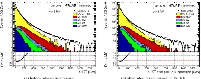
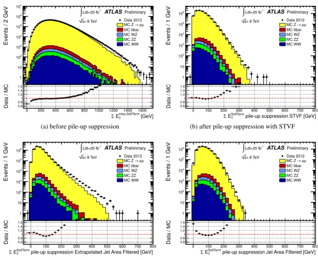
7.2.2 P

E

distributions in Z → `` events The distributions of P

E

for data are shown in Figure 6 for Z → µµ events. Some data-MC disagree- ment is observed in the P

E

distribution at values below ∼ 200 GeV and especially above ∼ 600 GeV before pile-up suppression, while the disagreement is larger after pile-up suppression, which has a large effect on the P

E

. The distributions of P

E

and of P

E

are shown in Figure 7 and 8, respec- tively. The discrepancy in the P

E

distribution is mainly due to the discrepancy in the P

E

because of the mis-modeling of the number of jets in the P OWHEG +P YTHIA 8 MC simulation of the hard pro- cess, while there is a better agreement in the P

E

distribution. The discrepancy observed in the P

E

distribution becomes more evident after pile-up suppression because of the strong pile-up suppression applied to the soft term.

0 200 400 600 800 1000 1200 1400 1600 1800

Events / 40 GeV

1 10 102

103

104

105

106

107

Data 2012 µ µ

→ MC Z MC ttbar MC WZ MC ZZ MC WW Ldt=20 fb-1

∫

= 8 TeV s

ATLASPreliminary

[GeV]

ET

Σ 0 200 400 600 800 1000 1200 1400 1600 1800

Data / MC ^0.6

0.81 1.2 1.4 1.6

(a) before pile-up suppression

0 200 400 600 800 1000 1200 1400 1600 1800

Events / 40 GeV

1 10 102

103

104

105

106

Data 2012 µ µ

→ MC Z MC ttbar MC WZ MC ZZ MC WW Ldt=20 fb-1

∫

= 8 TeV s

ATLAS Preliminary

pile-up suppression STVF [GeV]

ET

0 200 400 600 Σ800 1000 1200 1400 1600 1800

Data / MC ^0.6

0.81 1.2 1.4 1.6

(b) after pile-up suppression with STVF

0 200 400 600 800 1000 1200 1400 1600 1800

Events / 40 GeV

1 10 102

103

104

105

106

Data 2012 µ µ

→ MC Z MC ttbar MC WZ MC ZZ MC WW Ldt=20 fb-1

∫

= 8 TeV s

ATLASPreliminary

pile-up suppression Extrapolated Jet Area Filtered [GeV]

ET

Σ^{0 200 400 600 800 1000 1200 1400 1600 1800}

Data / MC ^0.6

0.8 1 1.2 1.4 1.6

(c) pile-up suppression Extrapolated Jet Area Filtered

0 200 400 600 800 1000 1200 1400 1600 1800

Events / 40 GeV

1 10 102

103

104

105

106

Data 2012 µ µ

→ MC Z MC ttbar MC WZ MC ZZ MC WW Ldt=20 fb-1

∫

= 8 TeV s

ATLAS Preliminary

pile-up suppression Jet Area Filtered [GeV]

ET

0 200 Σ400 600 800 1000 1200 1400 1600 1800

Data / MC ^0.6

0.8 1 1.2 1.4 1.6

(d) pile-up suppression Jet Area Filtered

Figure 6: Distribution of P

E

as measured in a data sample of Z → µµ events before pile-up suppres- sion (a), after pile-up suppression with the STVF (b), with the Extrapolated Jet Area Filtered (c) and with the Jet Area Filtered (d) methods. The expectation from Monte Carlo simulation is superimposed and normalized to data, after each MC sample is weighted with its corresponding cross-section. The lower parts of the figures show the ratio of data over MC.

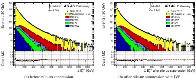
It is interesting to notice that using the A LPGEN MC event generator the data-MC agreement for the

P E

distribution improves, as shown in Figure 9, which is to be compared with Figure 6. This can be

0 200 400 600 800 1000 1200 1400 1600

Events / 20 GeV

1 10 102

103

104

105

106

107

Data 2012 µ µ

→ MC Z MC ttbar MC WZ MC ZZ MC WW Ldt=20 fb-1

∫

= 8 TeV s

ATLASPreliminary

[GeV]

jets

ET

Σ

0 200 400 600 800 1000 1200 1400 1600

Data / MC ^0.60.8

1 1.2 1.4 1.6

(a) before pile-up suppression

0 200 400 600 800 1000 1200 1400 1600

Events / 20 GeV

1 10 102

103

104

105

106

107

Data 2012 µ µ

→ MC Z MC ttbar MC WZ MC ZZ MC WW Ldt=20 fb-1

∫

= 8 TeV s

ATLAS Preliminary

after pile-up suppression [GeV]

jets

ET

Σ

0 200 400 600 800 1000 1200 1400 1600

Data / MC ^0.60.8

1 1.2 1.4 1.6

(b) after pile-up suppression with JVF

Figure 7: Distribution of P

E

computed from jets with p

> 20 GeV ( P

E

) before pile-up suppres- sion (a) and after pile-up suppression with JVF (b) for Z → µµ data. The expectation from Monte Carlo simulation is superimposed and normalized to data, after each MC sample is weighted with its corresponding cross-section. The lower parts of the figures show the ratio of data over MC.

explained by a more precise description of jet multiplicity with respect to P OWHEG +P YTHIA 8 which results in a better data-MC agreement for the P

E

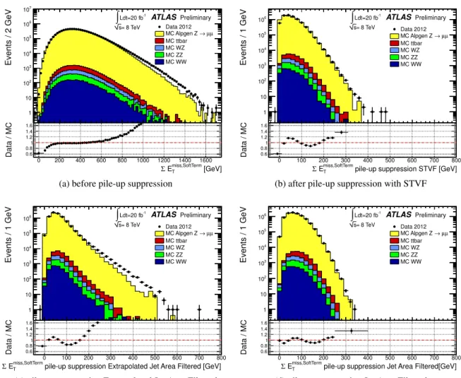
as shown in Figure 10, which is to be compared with Figure 7. Figure 11, which is to be compared with Figure 8, shows the distributions of P

E

using the A LPGEN MC. While before pile-up suppression there is a similar data-MC agreement as in Figure 8, which is expected because the soft term is dominated by the pile-up and the pile-up simulation is the same, after pile-up suppression there is a larger data-MC disagreement for A LPGEN , but this does not affect much the global P

E

distribution, due to the strong suppression of P

E

after pile-up.

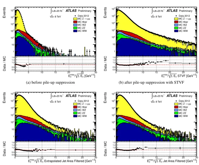
Finally, the distributions of the ratio E

/ √

Σ E

, are shown in Figure 12. This ratio is an interesting quantity because it has been used as an estimator of the E

significance in the absence of pile-up.

There is a data-MC agreement at the 20% level in the distributions of this ratio both before and after pile-up suppression.

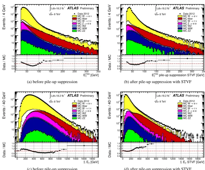
7.2.3 W → `ν events

In this section the E

performance is studied in W → `ν events. In these events genuine E

is expected due to the presence of the neutrino, therefore the E

scale can be checked.

The distributions of E

and P

E

in data and in MC simulation are shown in Figure 13 for W → eν events. There is a data-MC discrepancy in the E

distribution larger than that found in Z → µµ (shown in Figure 3), which may in part be due to the fact that the QCD background, which should predominantly populate the region of low E

, is not included in the MC expectations shown.

A discrepancy is also observed in the P

E

distribution.

7.3 E

T

resolution

A first study of the E

resolution is performed using the ratio:

R = RMS(E

/E

)/hE

/E

i (6)

0 200 400 600 800 1000 1200 1400 1600

Events / 2 GeV

1 10 102

103

104

105

106

107

Data 2012 µ µ

→ MC Z MC ttbar MC WZ MC ZZ MC WW Ldt=20 fb-1

∫

= 8 TeV s

ATLASPreliminary

[GeV]

miss,SoftTerm

ET

Σ

0 200 400 600 800 1000 1200 1400 1600

Data / MC ^0.6

0.81 1.2 1.4 1.6

(a) before pile-up suppression

0 100 200 300 400 500 600 700 800

Events / 1 GeV

1 10 102

103

104

105

106

Data 2012 µ µ

→ MC Z MC ttbar MC WZ MC ZZ MC WW Ldt=20 fb-1

∫

= 8 TeV s

ATLAS Preliminary

pile-up suppression STVF [GeV]

SoftTerm

ET

Σ

0 100 200 300 400 500 600 700 800

Data / MC ^0.6

0.81 1.2 1.4 1.6

(b) after pile-up suppression with STVF

0 100 200 300 400 500 600 700 800

Events / 1 GeV

1 10 102

103

104

105

106

Data 2012 µ µ

→ MC Z MC ttbar MC WZ MC ZZ MC WW Ldt=20 fb-1

∫

= 8 TeV s

ATLASPreliminary

pile-up suppression Extrapolated Jet Area Filtered [GeV]

SoftTerm

ET

Σ ^{0 100 200 300 400 500 600 700 800}

Data / MC ^0.6

0.8 1 1.2 1.4 1.6

(c) pile-up suppression Extrapolated Jet Area Filtered

0 100 200 300 400 500 600 700 800

Events / 1 GeV

1 10 102

103

104

105

106

Data 2012 µ µ

→ MC Z MC ttbar MC WZ MC ZZ MC WW Ldt=20 fb-1

∫

= 8 TeV s

ATLAS Preliminary

pile-up suppression Jet Area Filtered [GeV]

SoftTerm

ET

Σ

0 100 200 300 400 500 600 700 800

Data / MC ^0.6

0.8 1 1.2 1.4 1.6

(d) pile-up suppression Jet Area Filtered

Figure 8: Distribution of P

E

before pile-up suppression (a), corrected with STVF (b), corrected

with Extrapolated Jet Area Filtered (c) and corrected with Jet Area Filtered (d) for Z → µµ data. The

expectation from Monte Carlo simulation is superimposed and normalized to data, after each MC sample

is weighted with its corresponding cross-section. The lower parts of the figures show the ratio of data

over MC.