ATLAS-CONF-2013-005 26January2013
ATLAS NOTE
ATLAS-CONF-2013-005
January 20, 2013
Measurement of δ-rays in ATLAS silicon sensors
The ATLAS Collaboration
Abstract
In the inner detector of the ATLAS experiment at the LHC,
δ-rays originating from par-ticle interactions in the silicon sensors may cause additional hit channels. A method for identifying silicon hit clusters that are enlarged due to the emission of a
δ-ray is presented.Using pp collision data the expectation is confirmed that the
δ-ray production rate dependslinearly on the path length of the particle in silicon, independently of layer radius and detec- tor technology. The range of the
δ-rays, which is a property of the material and should notdepend on anything else, is indeed found to be constant as a function of detector layer, path length in silicon and momentum of the particle traversing the silicon. As a by-product of this analysis a method is proposed that could correct for the effect of these
δ-rays, and thiscould be used to improve track reconstruction.
c
Copyright 2013 CERN for the benefit of the ATLAS Collaboration.
Reproduction of this article or parts of it is allowed as specified in the CC-BY-3.0 license.
1 Introduction
Energy deposition by charged particles in silicon leads to the production of low energy secondary elec- trons, called δ-rays, that can travel distances of several hundred microns [1, 2]. They may produce hits in strips or pixels that were not traversed by the primary charged particle. These clusters including δ-ray hits broaden the cluster and bias the position measurement. We present a method to identify these δ-rays.
Using this method we measure the rate and range of the δ-rays in both data and Monte Carlo simulation.
We also measure the cluster centroid position bias in such clusters from the track residual distributions
1. When a track has been reconstructed, it is known to some precision which specific strips or pixels the particle has traversed. With this information the clusters can be re-examined to look for pixels or strips that registered a hit near the particle trajectory, but were not actually traversed by the particle. These clusters would be likely to include additional hits from δ-ray emission. However, the accuracy of the track reconstruction is not su
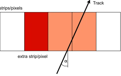
fficient to extrapolate exactly within strips or pixels. Instead, the track incidence angle projected on the r-φ plane, α, on each silicon layer is used to calculate the maximum number of strips or pixels that a particle should have crossed. This is a quantity that is precisely determined, and clusters wider than permitted by α are likely to include additional hits from δ-ray emission. A sketch of this can be seen in Fig. 1, where it is impossible, given the small α, that the particle in fact traverses three strips or pixels.
Another possible cause of cluster broadening is the merging of two clusters from di
fferent particles.
Merged clusters are simply the random overlap of two clusters from two different particles. They are indistinguishable from δ-rays on a cluster-by-cluster basis but their rate decreases with layer radius (be- cause of decreasing occupancy). Sometimes the presence of a merged cluster can be detected: this is the case whenever two or more reconstructed tracks share a cluster. If that is the case, that cluster can then be excluded from the δ-ray analysis.
Artificially enlarged clusters
Track strips/pixels
extra strip/pixel
1
α
could be dues to either delta ray or shared cluster
Figure 1: Sketch of a reconstructed particle track traversing two strips/pixels with an extra strip/pixel, which could be caused by either a merged cluster or a cluster broadened by δ-ray emission.
The production rate of δ-rays depends on how much silicon a charged particle traverses and therefore
1Throughout this note theunbiasedresidual is used, meaning that in the calculation of the track residual, the specific hit is excluded to prevent biasing of the track by the analyzed hit.
it is studied as a function of the three dimensional path length in silicon, which is a function of the particle η as well as α. The formula for this quantity is given in Section 2.5. The rate of δ-ray production is expected to change with the particle βγ according to the Bethe-Bloch formula [1] as described in Section 2.1. The generation of δ-rays should not depend on layer radius, or whether the layer is pixels or strips. Nevertheless, the data is studied as a function of both Pixel and SCT detector layer to test this expectation.
In order to fit the data and study how δ-ray production depends on the above parameters, the differ- ential probability for a particle to emit a δ-ray that travels a distance x along the r-φ-direction is modeled with Eq. 1.
dP
δ=AL
ρ e
−x/ρdx (1)
In Eq. 1, ρ is the range in the r-φ plane of the δ-rays to be determined. The integrated probability from x
=0 to x
=∞is the normalization AL, where the dependence on the path length in silicon L is explicitly shown since the δ-ray production must scale this way. Thus, the rate constant A has units of inverse distance. For convenience, A will be quoted in units of 1/300 µm since 300 µm is a standard thickness for silicon sensors.
This is an empirical model that is tested in Section 3.2. A derivation of the expected distribution from the known δ-ray energy spectrum and angular distribution was considered impractical because these must be integrated over the particle incidence angle and sensor tilt, taking into account the cuto
ffat the sensor face, and over energy loss along the path of the emitted electron, which is propagating in a magnetic field. This calculation is done by the ATLAS GEANT 4 simulation [3, 4], which is compared to the data and thus validated in this note.
The original purpose of this study was to check how accurately δ-ray effects are reproduced in the detector simulation. Then, having developed a method to measure δ-rays, it became evident that this information can be used to correct cluster positions once tracks have been reconstructed, and this would improve the track parameters in a second pass refit. In this note we describe the measurement of δ-rays in data and simulation and include results for measured cluster position bias.
2 Method
2.1 Data samples and track selection
The rate measurement is fundamentally one of counting. A sample of reconstructed tracks is defined, and then the number of clusters on these tracks that are consistent with being broadened by δ-ray emission is counted. This study is carried out in the last two barrel layers of the Pixel detector and in the SCT barrel layers. The first Pixel detector layer is excluded, since the track extrapolation is worse there, due to the fact that the extrapolation is only ”anchored” on one side. This leads to a wider residual distribution with longer tails than for the other layers. This selection simplifies the analysis and yields the best quality tracks. Since a universal property of the passage of particles through silicon is measured, these cuts can be used without biasing the results.
The analysis is carried out with data taken with the ATLAS detector [5] from July to August 2010, with about 257 million events. About 300 million events simulated using the ATLAS GEANT4 im- plementation [3, 4] with a GEANT δ-range cut of 50 µm are used as simulation sample. This sample contains 8 interactions per simulated beam crossing, but shared clusters are eliminated in the analysis, and no contamination by merged clusters is observed (more discussion can be found in Section 3.2).
Tight track quality cuts are applied as this is a relative measurement, and the e
fficiency of the track
selection is not important. All track quality cuts are shown in Table 1. No cut is made on the type of
particle that creates the δ-rays. From the Monte Carlo simulation, we find that about 67% of the particles are pions, 17% kaons and 12% protons. Because, according to the Bethe-Bloch formula the energy loss depends only on a particle’s βγ, the fraction of δ-rays caused by pions, kaons and protons respectively will differ for different momentum regions. The expected momentum dependence of the δ-ray rate can thus be calculated from the sum of the particle type fraction
×energy loss. From this calculation, it is expected that for three momentum bins 0.5 < p < 0.75 GeV, 0.75 < p < 1.25 GeV, p > 1.25 GeV, the relative rate of δ-rays normalized to the first momentum bin should scale as 1/0.9/0.88.
In order to give more reliable track reconstruction and residual distributions, a momentum cut of p >
1 GeV is introduced. However, this cut is loosened to 0.5 GeV when the p dependence is analyzed.
track selection cuts p
≥0.5 GeV (or 1 GeV)
χ
2/dof≤10
|z0| ≤
75 mm
|d0| ≤
5mm
|η| ≤
1.15
require at least 10 TRT hits require no shared cluster on track
Pixel detector residuals track selection SCT residual track selection at least 3 pixel hits at least 8 SCT hits
no pixel holes hit in the first layer cluster width in z
≤2
no ganged pixels
Table 1: Analysis selection cuts. Here, d
0and z
0are the transverse and longitudinal track impact pa- rameters relative to the coordinate origin (not the event primary vertex), where z measures longitudinal distance along the beam direction. η is the track pseudorapidity.
2.2 Expected cluster width W
eUsing the incidence angle α and the Lorentz drift angle, the “expected width” W
eof the cluster in the r-φ-plane is calculated according to Eq. 2. This is a signed variable in units of distance, the sign of α being preserved. This means that the information of whether a track crossed the detector left-to-right or right-to-left is kept. This is the physical extent of the charge deposition reaching the surface of the sensor, and should be independent of sensor segmentation. Its geometrical meaning is shown in Fig. 2.
W
e=t[ tan α
−tan λ] (2)
In Eq. 2, t is the sensor thickness (250 µm in Pixel [5] and 285 µm in SCT [5]) and λ is the Lorentz drift angle, which has a magnitude of about
−4◦in the SCT detector and 12
◦in the Pixel detector.
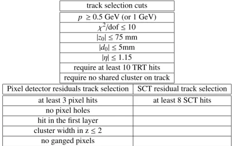
Sample distributions of W
efrom the large set of simulated events are shown in Fig. 3. Note that
the tilt of the detector with respect to the radial direction (−20
◦for the Pixel detector, 11
◦for the two
inner SCT layers, 11.25
◦for the two outer ones) does not exactly compensate for the Lorentz drift, and
therefore particles curved in one direction (i.e. with one charge) will have, on average, smaller
|We|than
those curved in the other direction. The two peaks thus correspond to positive and negative particles,
and their separation increases with layer number, since the particles get more curved the farther they are
from the interaction point.
Track
detector thickness (t) Wo = We
t x tan(λ) t x tan(α)
α
λ
Path Length L
We
α
λ
δ-ray
Wo
Expectation from track alone Expectation from track with δ-ray x
Figure 2: Sketch of the geometric meaning of W
oand W
ewith and without δ-rays. Only the 2 dimensional projection of the 3 dimensional path length L is shown. Here, x is the distance traversed by a particular δ-ray as described in Eq. 1
m in µ We
-250 -200 -150 -100 -50 0 50 100
m µ Entries / 10
0 50 100 150 200 250 300 350 400 450
103
×
SCT layer 3 SCT layer 2 SCT layer 1 SCT layer 0
ATLAS simulation preliminary
Figure 3: Distribution of W
efor the 4 SCT barrel layers in simulated data, for track momentum range
0.5< p <1.0 GeV.
To identify clusters likely to include δ-ray emission, hits for which
|We|is less than the strip (pixel) pitch of 80 µm (50 µm) are selected. This means that the charge from the primary particle can extend over at most 2 strips (pixels), and therefore clusters of observed cluster width (W
o) greater than 2 strips or pixels must arise from either δ-rays or merged clusters, the increase of cluster size due to noise being negligible [6].
2.3 Shifted residual distribution
The number of δ-ray clusters is now counted in bins of W
o. To be consistent with Eq. 1, only single
δ-ray clusters should be counted, excluding multiple δ-rays and other possible backgrounds. A single
δ-ray adds a number of strips or pixels to only one side of a charge cluster. In a binary system, this leads to a discrete shift of the calculated cluster centroid. The shift of the residual distribution is expected to have a magnitude of approximately (W
o ×strip/ pixel pitch
−W
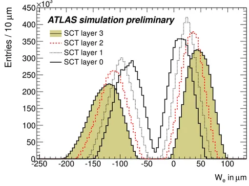
e)/2 (negative and a positive peaks corresponding to δ-rays traveling to left or right). Sample distributions of residuals for SCT clusters of di
fferent W
o, but always
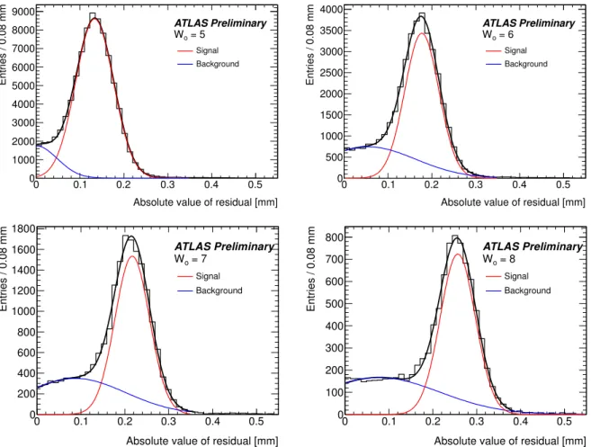
|We|< 80 µm are shown in Fig. 4. Further study of the residual structure is described in Section 4. The number of single delta-ray clusters in a given W
obin is the number of events in the shifted residual peaks (signal peaks), and can now be determined.
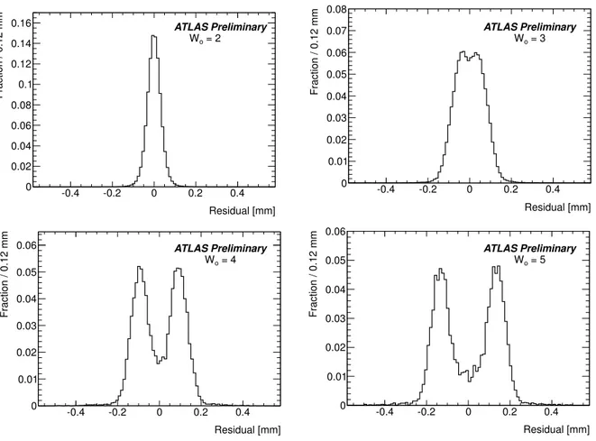
This is done by fitting the residual distribution to two Gaussians, one for the signal peak shifted away from zero, and the other for the background, having a mean near zero. This background is expected to contain multiple δ-ray events (which can lead to zero or a large residual displacement) as well as any other backgrounds not explicitly understood (the modeling of the background by a single Gaussian will be covered by a systematic uncertainty). A double Gaussian fits the observed distributions well, yielding a typical χ
2/do f between 1.5 and 1.8 for different bins in the variables described below. Fitting the residual magnitude rather than the signed residuals assumes the signal peak shifts are symmetric about zero, which is empirically verified in Section 4. Sample fits to residual magnitude distributions are shown in Fig. 5.
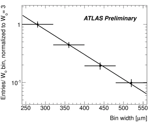
An example distribution of single δ-rays (i.e. the areas of the signal Gaussians seen in Fig. 5) vs. W
oin µm is shown in Fig. 6. An exponential fit to determine the range is superimposed and further discussed in Section 2.5. Only bins W
o> 3 for the SCT detector and W
o> 4 for the Pixel detector are fitted to the exponential, because the signal peaks in the W
o=3 (as well as W
o=4 in the Pixel detector) are not well resolved, having a mean close to 0, leading to a large uncertainty in the background component. The reason one more W
obin is excluded in the Pixel detector is that the Pixel sensors pitch is smaller than the SCT sensors, such that the shift of the residual Gaussian is reduced. An additional reason for excluding W
o =3 is that uncertainties in the W
ecalculation as well as electronic charge sharing effects could lead to an added background in that bin. Those effects are not due to charge sharing between Pixels/Strips on the front-end electronics, but between two neighboring implantations.
2.4 Merged Clusters
Merged clusters occur when the charge deposits from two separate particles overlap and are seen as a single cluster. For each of the two tracks, this will lead to added hits on one side only of the true cluster from that track, which will shift the residual distribution the same way as single δ-rays. The track reconstruction flags tracks that share at least one cluster with another track. Is is assumed that any cluster shared between two tracks consists in reality of merged clusters. We therefore remove merged clusters from the δ-ray sample by excluding such flagged tracks. The fraction of excluded tracks, after all our other selection cuts including the presence of a δ-ray candidate cluster, is 1.89%± 0.02% (1.46%±0.01%) for data (simulation).
To check the contamination by merged clusters, we exploit the fact that, unlike δ-rays, the number of
merged clusters must scale with occupancy, which in turn scales with the number of tracks per event. We
Residual [mm]
-0.4 -0.2 0 0.2 0.4
Fraction / 0.12 mm
0 0.02 0.04 0.06 0.08 0.1 0.12 0.14 0.16
o = 2 W
ATLAS Preliminary
Residual [mm]
-0.4 -0.2 0 0.2 0.4
Fraction / 0.12 mm
0 0.01 0.02 0.03 0.04 0.05 0.06 0.07 0.08
o = 3 W
ATLAS Preliminary
Residual [mm]
-0.4 -0.2 0 0.2 0.4
Fraction / 0.12 mm
0 0.01 0.02 0.03 0.04 0.05 0.06
o = 4 W
ATLAS Preliminary
Residual [mm]
-0.4 -0.2 0 0.2 0.4
Fraction / 0.12 mm
0 0.01 0.02 0.03 0.04 0.05 0.06
o = 5 W
ATLAS Preliminary
Figure 4: Normalized distributions of residuals in data for the SCT detector innermost layer clusters on tracks with
|We|< 80 µm and a path length in the silicon sensor between 275 and 320 µm, for di
fferent W
ovalues.
split our samples for rate and range determination in two bins of < 60 and > 60 tracks
/event. Following the analysis described later, the rate constant A from Eq. 1 is found to be 1.54
±0.11 % (1.59
±0.10 %) in data and 1.19
±0.12 % (1.13
±0.11 %) in simulation, for < 60 (> 60) tracks
/event for the SCT detector. For the Pixel detector, the results are 1.54
±0.15 % (1.73
±0.18 %) in data and 1.66
±0.42 % (1.46
±0.17 %) in simulation, for < 60 (> 60). Errors are statistical only. If there were a significant residual contamination of merged clusters, it should translate into a higher rate for the samples with more tracks
/event. The consistency of the results supports the assertion that residual contamination due to merged clusters is negligible. We note that the mean number of tracks/event in our samples is 63 for data and 112 for simulation. The simulation used has a fixed pileup of 8 interactions per event, whereas the pileup in data varies according to instantaneous luminosity.
2.5 Range and Rate determination
Eq. 1 can be integrated to obtain N
δ(w
o, b) in Eq. 3, the expected number of single δ-rays in a number
b of consecutive W
obins starting at W
o =w
o. In the analysis, w
o =4 and b
=3 is used for the SCT
detector, meaning that the number of single δ-rays for W
o=4 , 5 and 6 are used, and N
δis thus the sum
of the single δ-rays of all three W
obins. As described above, the W
o =4 bin is not used in the Pixel
detector, and thus w
o =5 and b
=3 there (going up to W
o=7). The reason that b
=3 is used is that for
Absolute value of residual [mm]
0 0.1 0.2 0.3 0.4 0.5
Entries / 0.08 mm
0 1000 2000 3000 4000 5000 6000 7000 8000 9000
o = 5 W
ATLAS Preliminary
Signal Background
Absolute value of residual [mm]
0 0.1 0.2 0.3 0.4 0.5
Entries / 0.08 mm
0 500 1000 1500 2000 2500 3000 3500 4000
o = 6 W
ATLAS Preliminary
Signal Background
Absolute value of residual [mm]
0 0.1 0.2 0.3 0.4 0.5
Entries / 0.08 mm
0 200 400 600 800 1000 1200 1400 1600 1800
o = 7 W
ATLAS Preliminary
Signal Background
Absolute value of residual [mm]
0 0.1 0.2 0.3 0.4 0.5
Entries / 0.08 mm
0 100 200 300 400 500 600 700 800
o = 8 W
ATLAS Preliminary
Signal Background
Figure 5: Distribution of residual magnitude in data for all SCT layers combined, for clusters on tracks with
|We|< 80 µm, path length in silicon between 275 and 450 µm, and p >1 GeV. Distribution are fit to sum of a background Gaussian and a signal Gaussian as described in the text. The component Gaussians as well as their sum as returned by the fit are superimposed on the plots. The χ
2/do f for all four fits is about 1.15.
higher W
obins, the statistics are low, and the fits to the residual distributions are not very robust.
N
δ(w
o, b)
=N
1AL ρ
Z (wo−3/2+b)s
(wo−3/2)s
e
−x/ρdx
+N
2AL ρ
Z (wo−2+b)s (wo−2)s
e
−x/ρdx (3) In Eq. 3, N
1(N
2) is the number of particles crossing one (two) pixels or strips, and s is the pixel or strip pitch. The first term is the contribution from particles crossing one pixel or strip, which would lead to one hit clusters in the absence of δ-rays. Similarly, the second term is the contribution from tracks crossing two pixels or strips. The total number of tracks is N
=N
1+N
2, since the
|We|< s selection excludes tracks crossing more than two strips or pixels, which is the case for α < 12.2
◦in the SCT detector and α < 23.4
◦in the Pixel detector. The integral is a single exponential in w
o(Eq. 4),
N
δ(w
o, b)
=NALe
−wos/ρe
2s/ρ(1
−e
−bs/ρ)( N
1N e
−s/2ρ+N
2N ) (4)
Typically, AL is solved for in bins of detector layer, track momentum and path length in silicon, L, as
given by Eq. 5. The θ and η are the track polar angle and pseudorapidity, respectively. Eq. 5 is an
approximation valid for small tilt angles of the detector and planes parallel to the z-axis. Corrections to
µ m]
Bin width [ 250 300 350 400 450 500 550
= 3
obin, normalized to W
oEntries/ W
10
-11
ATLAS Preliminary
Figure 6: Distribution normalized to first bin of the δ-ray signal (from fit to residual peaks) in bins of W
ofor SCT. Here, p > 1.5 GeV, 320< L <380 µm and
|We|< 80 µm. Exponential fit of p
0×e
xp1for W
o> 3 is superimposed. Here, ρ
=1/ p
1.
this formula are found to be at the few % level for the ATLAS silicon detectors and are not considered further.
L
=t
psec
2α
+cot
2θ
=t
psec
2α
+(e
η−e
−η)
2/2 (5) In each of these bins, the Gaussian fits as shown in Fig. 5 are performed to get the number of single δ-rays in different W
obins and they are then plotted as in Fig. 6. The range ρ of the single δ-ray is the inverse of the slope in Fig. 6. This, together with N, the total number of bins of all W
othat pass the W
e< s cut, makes it possible to solve Eq. 4 for AL. The results for A in units of 1/300 µm and ρ are presented in the following section.
The fractions of particles crossing one or two strips or pixels, N
1/N and N
2/N, are not directly observed. The number of observed 1-hit clusters, M
1, is given by N
1reduced by δ-ray emission, while the number of observed 2-hit clusters, M
2, is given by N
2both reduced by δ-ray emission and increased by feed-down from N
1. This is expressed in Eq. 6.
M
1 =N
1−AL ρ
Z ∞
s/2
e
−x/ρdx M
2 =N
2+AL
ρ
Z 3s/2
s/2
e
−x/ρdx
−AL ρ
Z ∞
s
e
−x/ρdx
(6)
Assuming the δ-ray terms in Eq. 6 are small, we use the following approximations:
N
1N
=M
1( M
1+M
2) , N
2N
=M
2(M
1+M
2) (7)
The validity of these approximations will be checked in Sec. 3.2. We note that to first order N
1/N and N
2/N are purely geometric and could be calculated from first principles. A track with W
e =0 has an infinitesimal probability of crossing two strips or pixels (it must pass exactly on the boundary), while a particle where W
eis just equal to the strip/pixel pitch (s) has an infinitesimal probability of falling in only one strip or pixel. In practice, there are corrections to this purely geometrical model due to charge diffusion, which makes W
e=0 impossible, electronic threshold which makes single strip or pixel clusters more likely, etc. This is why we choose to use the approximations in Eq. 7.
3 Results for Rate and Range
3.1 Layer dependence
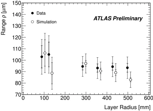
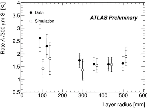
Figures 7 and 8 show the rate A and the range ρ as a function of detector layer. The data are integrated from L
=275 to 450 µm. They show that A is consistent with being the same within each sub detector, and that ρ is consistent with being the same everywhere, as expected. However, for data the rate parameter, A, is apparently decreasing with radius (or simply higher in the pixel detector than in the SCT). While merged clusters do have a falling rate with radius, we have shown in Sec. 2.4 that contamination from merged clusters is negligible. It is believed that this is likely a fluctuation in the residual fits, because when the data are combined for both layers and the momentum cut is relaxed to 0.5 GeV, both of which increases statistics, the discrepancy goes away, as will be seen in Sec. 3.3.
The apparent trend of falling Rate with detector layer can also be interpreted as a di
fference in central values between the Pixel and SCT detectors. This di
fference is plausible on physical grounds, because what is measured is an empirical rate, not a fundamental quantity: the Rate constant measured is a convolution of δ-ray emission with δ-ray propagation and detection in the sensor. While δ-ray emission is a physical process that should not di
ffer between the Pixel detector and the SCT, the two detectors have different Lorentz drift angles, different charge detection thresholds and opposite sensor tilts. This may cause a di
fference in measured Rate between the two detectors.
This makes it possible to separately combine all SCT and all pixel layers to increase statistics in the rest of the analysis. Note that for all following plots, the simulation x-axis value has been artificially shifted by a small o
ffset in the positive x-direction to visually separate the points.
3.2 Systematic uncertainties and quality control
A total of 284 Gaussian fits are used to determine A and ρ in di
fferent bins of layer, L and p. It is found that the lower the ratio of signal Gaussian to total area is, the larger the uncertainty in the fit becomes, since the model of a background Gaussian centered at or near 0 is only an approximation and the error introduced by it increases as the fraction of the background to total area increases. This leads to larger errors in the Pixel detector, where the signal fraction (defined as the ratio of signal area Gaussian over total area) varies from 0.5 to 0.6 for data and simulation, while the signal fraction is about 0.7 to 0.9 in data (0.6 to 0.75 for simulation) for the SCT detector. The signal fraction is between 0.14 and 0.25 in the first layer (L0) of the Pixel detector for p > 1.0 GeV. For 0.5 < p < 1.0 GeV in the Pixel detector layers 1 and 2, this fraction is between 0.15 and 0.27. This low signal to background is the reason for excluding these data from our measurements.
After determining A and ρ, it can now be verified that the approximation made for
NN1and
NN2is valid.
In order to do this, we pick sample values for N
1and N
2and calculate M
1and M
2from Eq. 6. We
then compare our estimated
NN1and
NN2(Eq. 7) to their true values. Using several different bins of L and
momentum as well as both Pixel and SCT detectors, and using the calculated A and ρ, it is found that
the error made in the approximation is of order 3% for the Pixel detector and of order 2% for the SCT
detector. This is treated as a systematic error.
Layer Radius [mm]
0 100 200 300 400 500 600
m] µ [ ρ Range
70 80 90 100 110 120 130 140 150
ATLAS Preliminary
Data Simulation
Figure 7: Range measurement for data and simulation samples, shown as function of layer radius, with p > 1 GeV averaged over three path length bins 275 < L < 320 µm, 320 < L < 380 µm, 380 < L <
450 µm. The inner error bars show the statistical uncertainty only, the outer error bars show the statistical and systematic uncertainties combined. The simulation points are artificially shifted by 15 mm for better distinction.
Another source of systematic error is the di
fferent results for ρ for di
fferent layers, L and momentum bins, despite the expectation that it be a property of silicon alone. Analyzing the differences in different bins, this discrepancy is estimated to be of the order of 3.5% for the SCT detector and 2% for the Pixel detector. Here, the variance from the mean ρ of di
fferent measured ρ values was used. It was computed separately for the Pixel and the SCT detectors.
The single exponential hypothesis, that one slope parameter ρ fits the data well is verified by fitting only part of the data at a time, starting at a given W
obin and including only large W
obins in the fit. Fig. 9 shows the ρ value obtained vs. the fit starting point in µm. This is evidence that the single exponential hypothesis is good within the above systematic errors.
We expect that a small amount of the charge deposited in one channel will be recorded in its neighbors due to inter-channel capacitance coupled with a finite integration time. Since no such e
ffect is included in the simulation and we do not have a quantitative estimate for it, we neglect it in our model. A future dedicated study to quantify this e
ffect would be of general interest. Such “electronic charge sharing” will smear the boundaries between W
obins.
The other main source of systematic error is that the double Gaussian fit does not perfectly model the background, since it is constituted of a variety of di
fferent sources, including non-recognized merged clusters and multiple δ-rays. Comparing fits and errors for, for instance, di
fferent means of the back- ground Gaussian, this error is estimated to be of the order of 5%.
A summary of the systematic uncertainties is shown in Table 2.
Layer radius [mm]
0 100 200 300 400 500 600
m Si [%] µ /300 A Rate
0.5 1 1.5 2 2.5 3 3.5 4
ATLAS Preliminary
Data Simulation
Figure 8: Rate measurement for data and simulation samples, shown as function of layer radius, with p
> 1 GeV averaged over three path length bins 275 < L < 320 µm, 320 < L < 380 µm, 380 < L <
450 µm. The inner error bars show the statistical uncertainty only, the outer error bars show the statistical and systematic uncertainties combined. The simulation points are artificially shifted by 15 mm for better distinction.
Sources of the systematic uncertainty on rate and range Pixel SCT
discrepancies in measured ρ 2% 3.5%
fit uncertainty of background 5% 5%
Total systematic error on range 5.3% 6.1%
Additional source of systematic uncertainty on rate Pixel SCT
N
1/N approximation 3% 2%
Total systematic error on rate 6.2% 6.4%
Table 2: Systematic uncertainties in rate and range 3.3 Momentum and path length results
The data for the SCT detector is divided into three momentum bins (0.5 < p < 0.75 GeV, 0.75 <
p < 1.25 GeV, p > 1.25 GeV) and three path length bins (275 < L < 320 µm, 320 < L < 380 µm,
380 < L < 450 µm), and combined in di
fferent ways to get measurements of the L and momentum
dependence of both A and ρ. Because there are fewer layers and thus lower statistical precision, the Pixel detector samples are separated into only two momentum bins (0.5 < p < 1.25 GeV, p > 1.25 GeV) and two path length bins (275 < L < 350 µm, 350 < L < 450 µm). In the following plots, the coordinate on the horizontal axis is determined as the average value of the quantity (path length or momentum), and not simply the middle of each bin.
For both sub detectors, no path length L dependence is observed in either A (Rate per path length,
m]
at which fitting starts [ µ W
o150 200 250 300 350 400 450 500 550
m] µ [ ρ Range
40 60 80 100 120 140 160 180 200
ATLAS Preliminary
Data Pixel Data SCT
Figure 9: Measured range as function of starting point of exponential fit for both Pixel and SCT detector.
Horizontal axis shows W
o×strip/ pixel pitch. All layers included, p > 1 GeV and 275 < L < 450 µm.
m]
Path length in silicon [µ 280 300 320 340 360 380 400 420 440
m Si [%]µ /300 ARate
0.5 1 1.5 2 2.5 3 3.5 4
ATLAS Preliminary
Data Pixel Simulation Pixel
Figure 10: Rate measurement vs. path length L, p > 0.5 GeV, for both Pixel layers and data and sim- ulation, path length bins are 275 < L < 350 µm and 350 < L < 450 µm. The inner error bars show the statistical uncertainty only, the outer error bars show the statistical and systematic uncertain- ties combined. The simulation points are artificially shifted by 10 µm.
m]
Path length in silicon [µ 280 300 320 340 360 380 400 420 440
m Si [%]µ /300 ARate
0.5 1 1.5 2 2.5 3 3.5 4
ATLAS Preliminary
Data SCT Simulation SCT
Figure 11: Rate measurement vs. path length L, for all four SCT layers, for data and simulation sam- ples, p > 1 GeV. Path length bins are: 275 < L <
320 µm, 320 < L < 380 µm, 380 < L < 450 µm.
The inner error bars show the statistical uncertainty only, the outer error bars show the statistical and systematic uncertainties combined. The simulation points are artificially shifted by 10 µm.
Figs. 10 and 11) or ρ (Figs. 12 and 13), which agrees with the expectations that the rate scales linearly
with path length and the range is a property of silicon alone. Both data and simulation are consistent,
showing very good agreement over the entire path length range probed.
m]
Path length in silicon [µ 280 300 320 340 360 380 400 420 440
m]µ [ρRange
80 100 120 140 160 180 200
ATLAS Preliminary
Data Pixel Simulation Pixel
Figure 12: Range measurement vs. path length L, p > 0.5 GeV, for both Pixel layers and data and sim- ulation, path length bins are 275 < L < 350 µm and 350 < L < 450 µm. The inner error bars show the statistical uncertainty only, the outer error bars show the statistical and systematic uncertain- ties combined. The simulation points are artificially shifted by 10 µm.
m]
Path length in silicon [µ 280 300 320 340 360 380 400 420 440
m]µ [ρRange
80 100 120 140 160 180 200
ATLAS Preliminary
Data SCT Simulation SCT
Figure 13: Range measurement vs. path length L, for all four SCT layers, for data and simula- tion samples, p > 1 GeV. Path length bins are:
275 < L < 320 µm, 320 < L < 380 µm,
and 380 < L < 450 µm. The inner error bars show the statistical uncertainty only, the outer error bars show the statistical and systematic uncertain- ties combined. The simulation points are artificially shifted by 10 µm.
[GeV]
p
0.5 1 1.5 2 2.5
m Si [%] µ /300 A Rate
0.5 1 1.5 2 2.5 3 3.5 4
ATLAS Preliminary
Data SCT Simulation SCT
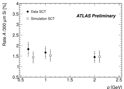
Figure 14: Results for rate per 300 µm path length as function of track momentum, 275 < L < 450 µm,
averaged over all four SCT layers. The inner error bars show the statistical uncertainty only, the outer er-
ror bars show the statistical and systematic uncertainties combined. The simulation points are artificially
shifted by 0.1 GeV.
Figure 14 shows the rate measured in different track momentum bins in the SCT detector. Mo- mentum and not transverse momentum is used because δ-ray production depends on a particle’s Lorentz boost βγ. As explained in Sec. 2.1, A should decrease by about 12% as function of increasing momentum in the given interval. This expectation is consistent with the measurements, although given the errors, it is not possible to resolve this 12% change. Figure 15 shows ρ measured in momentum bins. In this case there is no significant evidence of any change (no change is expected).
We do not examine the momentum dependence in the Pixel detector, because the signal to back- ground ratio of the residual distribution degrades significantly at low momentum. This is the same reason for which we excluded the Pixel detector layer 0 (L0) from the analysis (much lower signal to background ratio than for the other layers, see Sec. 3.2). We believe that the reason for the signal to background ratio degradation is the same for L0 and for low momentum in all Pixel layers: the track extrapolation error becomes large enough to dominate the residual, instead of the hit position error.
[GeV]
p
0.5 1 1.5 2 2.5
m] µ [ ρ Range
80 100 120 140 160 180
ATLAS Preliminary
Data SCT Simulation SCT
Figure 15: Results for range as function of track momentum, 275 < L < 450 µm, averaged over all four SCT layers. The inner error bars show the statistical uncertainty only, the outer error bars show the statistical and systematic uncertainties combined. The simulation points are artificially shifted by 0.1 GeV.
4 Measurement of Position Bias
The shift of the reconstructed cluster centroid depends on W
oas well as on W
e. Fig. 16 shows, for the SCT detector and W
o =6, the residual distribution as a function of W
ein a lego plot, and Fig. 17 shows the same plot for
|We|. There are two resolved peaks at smallW
e, merging at higher W
e, as the particular value of W
obecomes attainable by the particle alone, without the need for δ-rays to enlarge the cluster.
One can see a small bump in the residual distribution at 400 µm < W
e< 600 µm, this is due to the real 6-hit clusters. However, the total number of measured 6-hit clusters is completely dominated by δ-rays.
Empirically, it is found that such plots are symmetric in the sign of both W
eand residual. Therefore,
the plots can be folded onto the positive W
eand residual quadrant. Now, W
ecan be separated into bins and the residual can be fitted to two Gaussians, the “background Gaussian” and the “signal Gaussian”.
Fig. 18 shows a sample fit. The signal Gaussian is centered away from zero, and its mean is the average shift of the cluster centroid due to δ-rays in this W
eand W
obin.
µ m]
| in [
|W
e0 400 200
600 800
Residual [mm]
-0.4 -0.2
0 0.2 0.4 0
200 400 600 800 1000 1200 1400
ATLAS Preliminary
Figure 16: Lego plot of
|We|and residual for W
o=6 in the SCT detector.
These fits are made separately for the SCT and Pixel detectors, and the results for the means and widths of the signal Gaussians are collected in Figs. 19 and 20 (Figs. 21 and 22). The means show the expected behavior of decreasing with increasing W
e, and increasing with increasing W
o.
5 Conclusion and further work
This analysis has demonstrated a method for identifying δ-rays at the ATLAS detector at the LHC in pp-collisions, using the consistency between the observed cluster size and the expected size from the reconstructed track. It is found that the rate of δ-rays in ATLAS silicon is consistent with the expected dependence on path length in silicon and track momentum, and is the same for all silicon layers. This last property provides an important check that the signal sample is dominated by δ-rays and not randomly merged clusters, which would scale with hit occupancy and in turn with inverse layer radius. The same method is applied to Monte Carlo simulation and it is found that it agrees with the data for both the Pixel and the SCT detector. The SCT detector results have lower background and are therefore more precise that those for the Pixel detector.
This analysis exploits a characteristic shift of the track residual distributions caused by δ-rays or
merged clusters. This shift is measured as a function of observed and expected cluster sizes. Such
measurements, either parametrized or as a lookup table, could be used to correct the cluster centroid
position of hits that contain a δ-ray or a merged cluster. This would be particularly useful in the SCT
µm]
| in [
|We
0 200 400
600 Residual [mm] 800
0 0.1
0.2 0.3
0.4 0.5 0
200 400 600 800 1000 1200
ATLAS Preliminary
Figure 17: Lego plot of
|We|and magnitude of the residual for W
o=6 in the SCT detector.
detector, where the lack of charge information prevents the use of centroid finding algorithms prior to
track reconstruction.
Absolute value of residual [mm]
0 0.1 0.2 0.3 0.4 0.5
Entries/0.005 mm
0 100 200 300 400 500
600
ATLAS Preliminary
Figure 18: Typical fit for W
o=6 and
|We|centered around 19.6 µm.
m]
[ µ Mean W
e0 20 40 60 80 100 120 140 160 180 Mean of the residual distribution [mm] 0
0.05 0.1 0.15
0.2 0.25
ATLAS Preliminary
Wo = 3o = 4 W
o = 5 W
o = 6 W
Figure 19: Means of the residual Gaussian for SCT, p > 0.5 GeV.
µ m]
e
[ Mean W
10 20 30 40 50 60 70
Mean of the residual distribution [mm] 0 0.02 0.04 0.06 0.08 0.1 0.12 0.14
ATLAS Preliminary
o = 4 W
o = 5 W
o = 6 W
Figure 20: Means of the residual Gaussian for Pixel, p > 0.5 GeV.
µ m]
e
[ Mean W 0 20 40 60 80 100 120 140 160 180 Width of the residual distribution [mm] 0
0.01 0.02 0.03 0.04 0.05 0.06 0.07 0.08 0.09 0.1
ATLAS Preliminary
o = 3 W
o = 4 W
o = 5 W
o = 6 W
Figure 21: Width of the residual Gaussian for SCT, p > 0.5 GeV.
m]
[ µ Mean W
e10 20 30 40 50 60 70
Width of the residual distribution [mm] 0 0.01 0.02 0.03 0.04 0.05 0.06 0.07 0.08 0.09 0.1
ATLAS Preliminary
o = 4 W
o = 5 W
o = 6 W