The ATLAS Collaboration

ATLAS-CONF-2013-057 25June2013

ATLAS NOTE

ATLAS-CONF-2013-057

June 21, 2013

Search for long-lived stopped gluino R-hadrons decaying out-of-time with LHC collisions in 2011 and 2012 using the ATLAS detector

The ATLAS Collaboration

Abstract

R-hadrons are composite, massive, long-lived particles predicted in several scenarios of physics beyond the Standard Model, such as split supersymmetry. An updated search is per- formed for gluino R-hadrons which have come to rest within the ATLAS calorimeter, and decay at some later time to a gluon or q q ¯ pair and a neutralino. Candidate decay events are triggered in the empty bunch crossings of the LHC in order to remove pp collision back- grounds. Selections based on jet shape and muon-system activity are applied to discriminate events from cosmic ray and beam-halo muon backgrounds. In the absence of an excess, improved limits are set on the gluino mass, for di ff erent gluino decays, gluino lifetimes, and neutralino masses. With a neutralino of mass 100 GeV, the analysis excludes m

< 857 GeV (763 GeV expected), for a gluino lifetime between 10 µs and 1000 s in the generic R-hadron model with equal decays to q q ¯ χ ˜

and g χ ˜

.

⃝c Copyright 2013 CERN for the benefit of the ATLAS Collaboration.

Reproduction of this article or parts of it is allowed as specified in the CC-BY-3.0 license.

1 Introduction

Long-lived massive particles appear in many theories beyond the Standard Model [1]. They are predicted in R-parity conserving supersymmetry (SUSY) [2, 3, 4, 5, 6, 7, 8, 9, 10] models, such as split SUSY [11, 12] and gauge-mediated SUSY breaking [13, 14, 15, 16, 17, 18, 19], as well as other scenarios such as universal extra dimensions [20] and leptoquark extensions [21]. For instance, split SUSY addresses the hierarchy problem via the same fine-tuning mechanism that solves the cosmological constant problem;

SUSY can be broken at a very high energy scale, leading to heavy scalars, light fermions, and a light, finely tuned, Higgs particle [11]. Within this phenomenological picture, squarks will thus be much heavier than gluinos, suppressing the gluino decay. If the lifetime of the gluino is long enough, it will hadronize into R-hadrons, color-singlet states of R-mesons ( ˜ gq q), ¯ R-baryons ( ˜ gqqq), and R-gluinoballs ( ˜ gg ). While other models, notably R-parity violating SUSY, can produce a long-lived squark that would also form an R-hadron, the phenomenology is comparable to the gluino case but with a smaller production cross section [22, 23]. In this note the theoretical interpretation is limited to the gluino case.

R-hadron interactions in matter are highly uncertain, but some features are well predicted. The gluino can be regarded as a heavy, non-interacting spectator, surrounded by a cloud of interacting quarks. R- hadrons may change their properties through strong interactions with the detector. Most R-mesons will turn into R-baryons [24], and they can also change their electric charge through these interactions. At the Large Hadron Collider (LHC) at CERN [25], the gluino R-hadrons would be produced in pairs and approximately back-to-back in the plane transverse to the beam direction. Some fraction of these R- hadrons would lose all of their momentum, mainly from ionization energy loss, and come to rest within the detector volume, only to decay to a neutralino ( ˜ χ

) and a gluon or q q ¯ pair at some later time.

A previous search for stopped gluino R-hadrons was performed by the D0 collaboration [26] which excluded a signal for gluinos with masses up to 250 GeV. That analysis, however, could only use the filled crossings in the Tevatron bunch scheme and suppressed collision-related backgrounds by demanding that there was no non-di ff ractive interaction in the events. Search techniques similar to those described herein have also been employed by the CMS collaboration [27, 28] using 4 fb

of 7 TeV data under the assumptions that m

− m

> 100 GeV and BR( ˜ g → g χ ˜

) = 100%. The resulting limit, at 95% credibility level, is m

> 640 GeV for gluino lifetimes from 10 µs to 1000 s. ATLAS had up to now only studied 31 pb

of data from 2010 [29], resulting in the limit m

> 341 GeV, under similar assumptions.

This analysis complements previous ATLAS searches for long-lived particles [30, 31] which are less sensitive to particles with initial β ≪ 1. By relying primarily on calorimetric measurements, this analysis is also sensitive to events where R-hadron charge flipping may make reconstruction in the inner tracker and the muon system impossible. A potential detection of stopped R-hadrons could also lead to a measurement of their lifetime and decay properties. Moreover, the search is sensitive to any potential new physics scenario producing large out-of-time energy deposits in the calorimeter with minimal additional detector activity.

2 The ATLAS detector and event reconstruction

The ATLAS detector [32] consists of an inner tracking system (ID) surrounded by a thin superconducting solenoid, electromagnetic and hadronic calorimeters and a muon spectrometer (MS). The ID consists of silicon pixel and microstrip detectors, surrounded by a transition radiation straw-tube tracker. The calorimeter system is based on two active media for the electromagnetic and hadronic calorimeters:

liquid argon (LAr) in the inner and forward regions, and steel/scintillator tiles (TileCal) in the outer

barrel region, |η| < 1.7.

The calorimeters are segmented into cells which have typical size 0.1 by 0.1 in

η-ϕ space in the TileCal section. The MS, capable of reconstructing tracks within |η| < 2.7, uses toroidal bending fields generated by three large superconducting magnet systems. There is an inner, middle, and outer muon station, each consisting of several precision tracking layers. Local muon segments are first found in each station, before being combined into extended muon tracks.

For this analysis, events are reconstructed using “cosmic” settings for the muon system, to find muon segments with high e ffi ciency for muons which are “out-of-time” with respect to the expected time for a muon created from a pp collision traveling at the speed of light. Such out-of-time muons are also present in the two most important background sources. Cosmic ray muons are present at a random time compared to the bunch-crossing time. Beam-halo muons are in time with proton bunches but may appear early if they hit the muon chamber before particles created from the bunch crossing. Using cosmic settings for the muon reconstruction also loosens requirements on the segment direction and does not require the segment to point towards the interaction point.

Jets are constructed from clusters of calorimeter energy deposits using the anti-k

jet algorithm [33]

with the distance parameter set to R = 0 . 4, which assumes the energetic particles originate from the nom- inal interaction point. This assumption, while not generally valid, has been checked and still accurately quantifies the energy released from the stopped R-hadron decays occurring in the calorimeter, as shown by comparisons of test-beam studies with simulation [34]. Jet energy is quoted without correcting for the typical fraction of energy not deposited as ionization in the jet cone area, and the minimum jet p

is 7 GeV. ATLAS jet reconstruction algorithms are described in more detail elsewhere [35]. The missing transverse momentum (E

) is calculated from the transverse momenta of selected jets described above and all calorimeter energy clusters not associated to jets.

3 LHC bunch structure and trigger strategy

The LHC accelerates two counter-rotating proton beams, each divided into 3564 25 ns bunches. When protons are injected into the LHC, not every bunch is filled. During 2011 and 2012, alternate bunches within a “bunch train” were filled, leading to collisions every 50 ns, but there were also many gaps of various lengths between the bunch trains containing adjancent unfilled bunches. Filled bunches typically had > 10

protons. Unfilled bunches could contain protons due to di ff usion from filled bunches, but typically < 10

protons per bunch [36, 37]. The filled and unfilled bunches from the two beams can combine to make three different “bunch crossing” scenarios. A paired crossing consists of a filled bunch from each beam colliding in ATLAS and is when R-hadrons would be produced. An unpaired crossing has a filled bunch from one beam and an unfilled bunch from the other. Finally, in an empty crossing the bunches from both beams are unfilled.

Standard ATLAS analyses use data collected from the paired crossings, while this analysis searches for physics signatures of metastable R-hadrons produced in paired bunch crossings and decaying in the empty crossings. This is accomplished with a set of dedicated low-threshold calorimeter triggers which can fire only in the empty or unpaired crossings where the background to this search is much lower. The type of each bunch crossing is defined at the start of each LHC store using the ATLAS beam monitors [38].

ATLAS has a three-level trigger system consisting of one hardware and two software levels [39].

Signal candidates are collected using a hardware trigger requiring localized calorimeter activity, a so called jet trigger, with a 30 GeV transverse energy threshold. This trigger could fire only during an empty crossing at least 125 ns after the most recent paired bunch crossing, such that the detector is mostly free of background from previous interactions. The highest-level software trigger then requires a jet with transverse momentum, p

> 50 GeV, |η| < 1 . 3, and E

> 50 GeV. The software trigger is

upward. Cylindrical coordinates (r, ϕ) are used, ϕbeing the azimuthal angle around the beam pipe. The pseudorapidity is defined in terms of the polar angleθasη=−ln tan(θ/2).

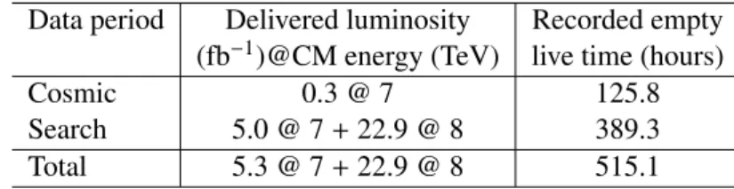
Table 1: The data analyzed in this work and the corresponding luminosity, energy, and live time of the ATLAS detector in empty bunch crossings during those periods.

Data period Delivered luminosity Recorded empty (fb

)@CM energy (TeV) live time (hours)

Cosmic 0.3 @ 7 125.8

Search 5.0 @ 7 + 22.9 @ 8 389.3

Total 5.3 @ 7 + 22.9 @ 8 515.1

more robust against detector noise, keeping the final trigger rate to < 1 Hz. After o ffl ine reconstruction, only 5% of events with more than two muon segments are saved, and no events with more than 20 muon segments are saved, to reduce the data storage needs. A data sample enriched with beam-halo muons is also collected with a lower-threshold jet trigger that fires in the unpaired crossings, and a sample is collected using a trigger that collects random events from the empty crossings to study background conditions.

4 Data samples

The data used are summarized in Table 1, where the corresponding delivered integrated luminosity and recorded live time in the empty bunches are provided. The early periods of data taking from 2011 are selected as a “cosmic background region” to estimate the rate of background events (mostly from cosmic ray muons, as discussed below). This is motivated by the low integrated luminosity and low number of filled bunches during these initial periods. For a typical signal model that this analysis excludes, < 3%

of events in the cosmic background region are expected to arise from signal processes. As discussed in detail in Section 7.2, the cosmic ray muon background rate is constant, but the signal production rate scales with luminosity. The later data of 2011 and all of 2012 is used as the “search region”, where an excess of events from R-hadron decays is searched for.

5 Simulation of R-hadrons

Monte Carlo simulations are used primarily to determine the reconstruction e ffi ciency and stopping frac- tion of the R-hadrons, and to study associated systematic uncertainties on the quantities used in the selections. The simulated samples have gluino masses in the range 400–1000 GeV, to which the present analysis is sensitive. The P ythia program [40], version 6.427, is used to simulate gluino-gluino pair pro- duction events. The string hadronization model [41], incorporating specialized hadronization routines [1]

for R-hadrons, is used to produce final states containing two R-hadrons.

To compensate for the fact that R-hadron scattering is not strongly constrained, the simulation of R- hadron interactions in matter is handled by a special detector response simulation [24] using G eant 4 [42, 43] routines based on several scattering / spectra models with different sets of assumptions: the Generic [24, 44], Regge [45, 46], and Intermediate [47] models. Each model makes di ff erent assumptions about the R-hadron nuclear cross section and mass spectra of various internal states. The models are:

Generic: Limited constraints on allowed stable states permit the occurrence of doubly charged R-

hadrons and a wide variety of charge-exchange scenarios. The scattering model is purely phase-

space driven. This model is chosen as the nominal signal model for gluino R-hadrons.

Regge: Only one (electrically neutral) baryonic state is allowed. The scattering model employs a triple- Regge formalism. This is expected to result in a lower stopping fraction than the Generic scenario.

Intermediate: As the name implies, the spectrum is more restricted than the Generic model, while still featuring charged baryon states. The scattering model used is that of the Generic model.

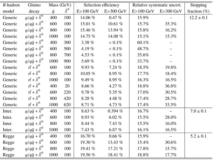
If a simulated R-hadron comes to rest in the ATLAS detector volume, its location is recorded. Table 2 shows the probability for a simulated signal event to have an R-hadron stop within the detector volume, for the models considered. The stopping fraction shows no significant dependence on the gluino mass within the statistical uncertainty of the simulation. Such an R-hadron would bind to a heavy nucleus of an atom in the detector, once it slows down su ffi ciently, and remain in place indefinitely [48]. These stopping locations are used as input into a second step of Pythia where the decays of the R-hadrons are simulated. A uniform random time translation is applied in a 25 ns time window, from − 15 to + 10 ns, relative to the bunch-crossing time, since the gluino will decay at a random time relative to the bunch structure of the LHC, but will be triggered on by ATLAS during the corresponding empty bunch crossing. These simulated events then proceed with the standard ATLAS digitization simulation [1] and event reconstruction (but with cosmic ray muon settings). The e ff ects of cavern background are not included in the simulation directly, but they are accounted for by measuring the muon activity in the random-triggered empty data (see section 9). The calorimeter activity due to preceding interactions is found to be negligible in the random-triggered data compared to the jet energy uncertainty and is ignored.

Di ff erent models allow the gluinos to decay via the radiative process, ˜ g → g χ ˜

, or via ˜ g → q q ¯ χ ˜

. The results are interpreted either assuming a 50% branching ratio to g χ ˜

and 50% to q q ¯ χ ˜

, or 100% to t t ¯ χ ˜

as would be the case if the top squark were significantly lighter than the other squarks. Reconstruction e ffi ciencies are typically ≈ 20% higher for q q ¯ χ ˜

compared to g χ ˜

decays. The neutralino mass, m

, is fixed to either 100 GeV, or such that there is just 100 GeV of free energy left in the decay (a compressed scenario).

6 Candidate selection

First, events are required to pass tight data quality constraints which verify that all parts of the detector are operating normally, and no calorimeter noise bursts are present in the event. The basic selection criteria imposed to isolate signal-like events from background events demand at least one high energy jet and no segments reconstructed in the muon system passing selections. Since most of the gluino bound states are produced centrally in η , the analysis uses only the central barrel of the calorimeter and requires that the leading jet satisfies |η| < 1.2. In order to reduce the background, the analysis demands the leading jet energy > 50 GeV. Up to five additional jets are allowed, more than expected for the signal models considered.

The fractional missing E

is the E

divided by the leading jet p

and is required to be > 0.5.

This eliminates background from beam-gas and residual pp events and has minimal impact on the signal e ffi ciencies. To remove events with a single, narrow spike in the calorimeter, due to noise in the elec- tronics or data corruption, events are vetoed where the smallest number of cells containing 90% of the energy deposit of the leading jet (n90) is fewer than four. This n90 requirement also reduces other back- ground significantly since most large energy deposits from muons in the calorimeter result from hard bremsstrahlung photons, which create short, narrow electromagnetic showers in the calorimeter. Large, broad, hadronic showers from deep-inelastic scattering of the muons off nuclei are far rarer. To further exploit the di ff erence between calorimeter energy deposits from muons and the expected signal, the jet width is required to be > 0.04, where jet width is the p

-weighted ∆ R average of each constituent from the jet axis and ∆R = √

∆η

+ ∆ϕ

. The fraction of the leading jet energy deposited in the TileCal must

Table 2: The selection e ffi ciency after all selections have been applied, its systematic uncertainty, and the stopping fraction, for all signal samples.

R-hadron Gluino Mass (GeV) Selection efficiency Relative systematic uncert. Stopping model decay g˜ χ˜⁰ E>100 GeV E>300 GeV E>100 GeV E>300 GeV fraction (%) Generic g/qq¯+χ˜⁰ 400 100 14.06 % 0.47 % 15.9% – 12.2±0.1 Generic g/qq¯+χ˜⁰ 600 100 15.01 % 10.61 % 15.7% 35.3%

Generic g/qq¯+χ˜⁰ 800 100 15.46 % 13.94 % 15.8% 16.2%

Generic g/qq¯+χ˜⁰ 1000 100 14.75 % 14.08 % 15.1% 15.3%

Generic g/qq¯+χ˜⁰ 400 300 3.38 % <0.1% 60.1% – Generic g/qq¯+χ˜⁰ 600 500 4.19 % <0.1% 48.7% – Generic g/qq¯+χ˜⁰ 800 700 4.53 % <0.1% 35.6% – Generic g/qq¯+χ˜⁰ 1000 900 5.69 % <0.1% 33.7% – Generic t¯t+χ˜⁰ 600 100 9.93 % 7.24 % 18.5% 19.8%

Generic tt¯+χ˜⁰ 800 100 10.05 % 8.95 % 17.7% 18.4%

Generic t¯t+χ˜⁰ 1000 100 9.49 % 8.95 % 16.3% 16.5%

Generic tt¯+χ˜⁰ 400 20 8.66 % 4.27 % 18.8% 36.8%

Generic t¯t+χ˜⁰ 600 220 9.78 % 5.35 % 17.0% 30.5%

Generic tt¯+χ˜⁰ 800 420 8.28 % 4.48 % 17.4% 28.7%

Generic t¯t+χ˜⁰ 1000 620 8.71 % 4.73 % 17.4% 33.5%

Inter. g/qq¯+χ˜⁰ 400 100 8.63 % 0.394 % 16.7% – 7.0±0.1 Inter. g/qq¯+χ˜⁰ 600 100 8.93 % 6.02 % 15.5% 28.0%

Inter. g/qq¯+χ˜⁰ 800 100 8.44 % 7.43 % 15.5% 16.0%

Inter. g/qq¯+χ˜⁰ 1000 100 7.43 % 6.87 % 16.1% 16.5%

Regge g/qq¯+χ˜⁰ 400 100 16.70 % 0.66 % 15.9% – 5.2±0.1 Regge g/qq¯+χ˜⁰ 600 100 19.30 % 13.43 % 15.4% 30.6%

Regge g/qq¯+χ˜⁰ 800 100 19.41 % 17.21 % 17.8% 15.7%

Regge g/qq¯+χ˜⁰ 1000 100 19.56 % 18.41 % 18.8% 17.7%

be > 0.5, to reduce background from beam-halo where the incoming muon can not be detected due to lack of MS coverage at low radius in the forward region.

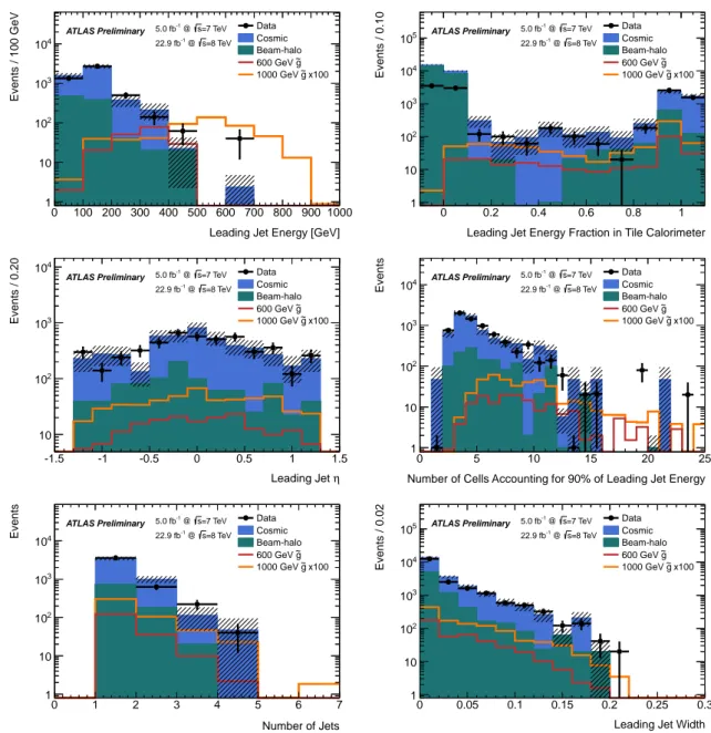
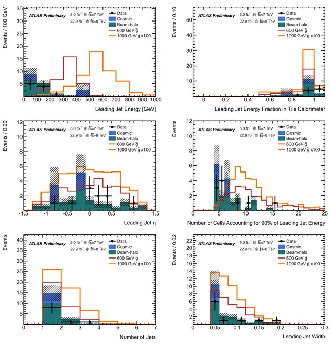
The analysis then requires that no muon segment that has more than four muon station measurements be reconstructed in the event. Muon segments with a small number of measurements are often present from cavern background, noise, and pile-up, as studied in the random-triggered data. The events before the muon segment veto and only requiring the leading jet energy > 50 GeV are studied as a control sample, since the expected signal to background is small. Comparisons of the distributions of several jet variables between backgrounds and data can be seen in Figure 1 for events in this control sample.

To remove overlap between the cosmic ray and beam-halo backgrounds in these plots, an event is not

considered “cosmic” if it has a muon segment with more than four hits and an angle within 0.2 radians

from parallel to the beamline. The same distributions are shown for events after the muon segment veto

in Figure 2. Finally, a leading jet energy requirement of > 100 or > 300 GeV defines two signal regions,

sensitive to either a small or large mass di ff erence between the gluino and neutralino in the signal model,

respectively. Table 2 shows the efficiencies of these selections on the signal simulations, and Table 3

presents the number of data events surviving each of the imposed selection criteria.

Leading Jet Energy [GeV]

0 100 200 300 400 500 600 700 800 900 1000

Events / 100 GeV

1 10 102

103

104

Data Cosmic Beam-halo

~g 600 GeV

x100 g~ 1000 GeV ATLAS Preliminary 5.0 fb^-1 @ s=7 TeV

=8 TeV s

-1 @ 22.9 fb

Leading Jet Energy Fraction in Tile Calorimeter

0 0.2 0.4 0.6 0.8 1

Events / 0.10

1 10 102

103

104

105

Data Cosmic Beam-halo

g~ 600 GeV

x100

~g 1000 GeV ATLAS Preliminary 5.0 fb^-1 @ s=7 TeV

=8 TeV s

-1 @ 22.9 fb

η Leading Jet

-1.5 -1 -0.5 0 0.5 1 1.5

Events / 0.20

10 102

103

104 _Data

Cosmic Beam-halo

~g 600 GeV

x100 g~ 1000 GeV ATLAS Preliminary 5.0 fb^-1 @ s=7 TeV

=8 TeV s

-1 @ 22.9 fb

Number of Cells Accounting for 90% of Leading Jet Energy

0 5 10 15 20 25

Events

1 10 102

103

104

Data Cosmic Beam-halo

g~ 600 GeV

x100

~g 1000 GeV ATLAS Preliminary 5.0 fb^-1 @ s=7 TeV

=8 TeV s

-1 @ 22.9 fb

Number of Jets

0 1 2 3 4 5 6 7

Events

1 10 102

103

104

Data Cosmic Beam-halo

~g 600 GeV

x100 g~ 1000 GeV ATLAS Preliminary 5.0 fb^-1 @ s=7 TeV

=8 TeV s

-1 @ 22.9 fb

Leading Jet Width

0 0.05 0.1 0.15 0.2 0.25 0.3

Events / 0.02

1 10 102

103

104

105

Data Cosmic Beam-halo

g~ 600 GeV

x100

~g 1000 GeV ATLAS Preliminary 5.0 fb^-1 @ s=7 TeV

=8 TeV s

-1 @ 22.9 fb

Figure 1: Jet variables for the empty bunch signal triggers. The requirements in Table 3 are applied

except for leading jet energy > 100 GeV and the muon segment veto. For the quantity being plotted,

its selection is not applied. Histograms are normalized to the expected number of events in the search

region. The hashed band shows the total statistical uncertainty on the background estimate.

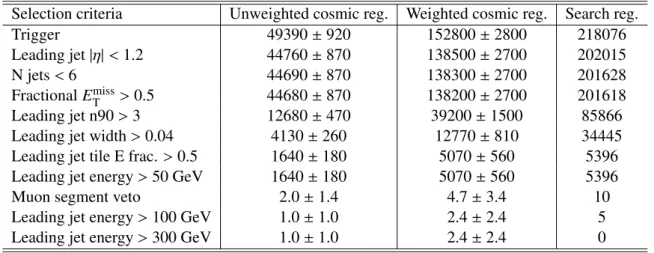
Table 3: Number of events after selections for data in the cosmic background and search regions, defined in Table 1. The cosmic background region data is shown before and after its scaling to the search region which accounts for the di ff erent detector live time and accidental muon segment veto e ffi ciency (if applicable) between the background and search regions. The uncertainties are statistical only.

Selection criteria Unweighted cosmic reg. Weighted cosmic reg. Search reg.

Trigger 49390 ± 920 152800 ± 2800 218076

Leading jet |η| < 1.2 44760 ± 870 138500 ± 2700 202015

N jets < 6 44690 ± 870 138300 ± 2700 201628

Fractional E

> 0.5 44680 ± 870 138200 ± 2700 201618

Leading jet n90 > 3 12680 ± 470 39200 ± 1500 85866

Leading jet width > 0.04 4130 ± 260 12770 ± 810 34445

Leading jet tile E frac. > 0.5 1640 ± 180 5070 ± 560 5396

Leading jet energy > 50 GeV 1640 ± 180 5070 ± 560 5396

Muon segment veto 2.0 ± 1.4 4.7 ± 3.4 10

Leading jet energy > 100 GeV 1.0 ± 1.0 2.4 ± 2.4 5

Leading jet energy > 300 GeV 1.0 ± 1.0 2.4 ± 2.4 0

7 Background Estimation

7.1 Beam-halo Background

Protons in either beam can interact with residual gas in the beampipe, or the beampipe itself if they stray o ff orbit, leading to a hadronic shower. If the interaction takes place several hundred meters from ATLAS, most of the shower is absorbed in shielding or surrounding material before reaching ATLAS.

The muons from the shower can survive and enter the detector, traveling parallel to the beamline and in time with the (filled) proton bunch [49, 50]. The unpaired-bunch data with a jet passing the criteria is dominantly beam-halo.

To estimate the number of beam-halo events in the empty bunches of the search region, an orthogonal sample of events from the unpaired bunch crossings is used to measure the fraction of beam-halo events which pass the jet criteria, but fail to have a muon segment identified. This fraction is then multiplied by the number of beam-halo events observed in the signal region that do have an identified muon segment to give the estimate of the number that should not have a muon segment and thus contribute to background in the signal region.

First beam-halo events in the unpaired bunch crossing data are tagged by applying a modified version of the search selection criteria. The muon segment veto is removed, events with leading jet energy

> 50 GeV are used, and the n90 requirement is not applied. Studies show that the muon e ffi ciency is not significantly correlated with the energy or shape of the jet in the calorimeter for beam-halo events.

A muon segment is required to be nearly parallel with the beam pipe, θ < 0.2 or θ > (π − 0.2), and

have more than four muon station measurements. Secondly beam-halo events that failed to leave a muon

segment are tagged. This allows the fraction of beam-halo events with no muon segment identified to be

calculated. Then the number of beam-halo muons in the search region (the empty bunches) that did leave

a muon segment is calculated. The same selection criteria as listed in Table 3 is used, excluding the 100

GeV requirement. However instead of a muon segment veto a parallel segment is required. If no events

are present, the uncertainty is taken as ±1 event. Findings are summarized in Table 4.

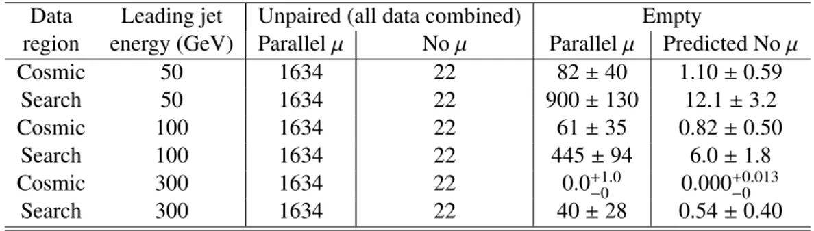
Table 4: Estimation of beam-halo events entering the search region, as described in section 7.1. The fraction of beam-halo muons that do not leave a segment is calculated from the unpaired data. This fraction is then applied to the number of events in the search region where a segment was reconstructed to yield a beam-halo estimation. The quoted uncertainties are statistical only.

Data Leading jet Unpaired (all data combined) Empty

region energy (GeV) Parallel µ No µ Parallel µ Predicted No µ

Cosmic 50 1634 22 82 ± 40 1.10 ± 0.59

Search 50 1634 22 900 ± 130 12.1 ± 3.2

Cosmic 100 1634 22 61 ± 35 0.82 ± 0.50

Search 100 1634 22 445 ± 94 6.0 ± 1.8

Cosmic 300 1634 22 0.0

0.000

Search 300 1634 22 40 ± 28 0.54 ± 0.40

7.2 Cosmic Ray Muon Background

The background from cosmic ray muons is estimated using the cosmic background region (described in Section 4). The beam-halo background is estimated for this data sample as above, and this estimate is subtracted from the observed events passing all selections. Finally, this number of cosmic ray events in the cosmic region is scaled according to the ratio of live times of the signal region / cosmic region to estimate the cosmic ray background in the signal region. Additionally, the cosmic background estimate is multiplied by the muon-veto e ffi ciency (see Sec. 9) to account for the rejection of background caused by the muon veto.

8 Event Yields

Distributions of jet variables are plotted for events in the signal regions after applying all selection criteria and compare to the estimated backgrounds in Figure 3. The shapes of these distributions and event yields agree well. Table 5 shows the signal region event yields and background estimates, which show that there is no evidence for excess signal candidates.

9 Contributions to Signal E ffi ciency

Quantifying the signal e ffi ciency for the stopped gluino search presents several unique challenges due to the non-prompt nature of their decays. Specifically there are four sources of inefficiency: stopping fraction (Section 5), reconstruction e ffi ciency (Table 2), accidental muon veto, and probability to have the decay occur in an empty bunch crossing (timing acceptance). Since the first two have been discussed above, here only on the accidental muon veto and timing acceptance are described.

9.1 Accidental Muon Veto

Operating in the empty bunch crossings has the significant advantage of eliminating collision back-

grounds. However because such a stringent muon activity veto is employed, a significant number of

events are rejected in the o ffl ine analysis from spurious segments in the muon system, which are not

properly modeled in the MC signal simulation. Both β-decays from activated nuclei and δ-rays could

produce segments with more than four muon station measurements. This is a separate e ff ect from a signal

decay producing a muon segment which then vetoes the event. To study the rate of muon segments we

Leading Jet Energy [GeV]

0 100 200 300 400 500 600 700 800 900 1000

Events / 100 GeV

5 10 15 20 25 30 35

Data Cosmic Beam-halo

~g 600 GeV

x100 g~ 1000 GeV ATLAS Preliminary 5.0 fb^-1 @ s=7 TeV

=8 TeV s

-1 @ 22.9 fb

Leading Jet Energy Fraction in Tile Calorimeter

0 0.2 0.4 0.6 0.8 1

Events / 0.10

10 20 30 40 50

Data Cosmic Beam-halo

g~ 600 GeV

x100

~g 1000 GeV ATLAS Preliminary 5.0 fb^-1 @ s=7 TeV

=8 TeV s

-1 @ 22.9 fb

η Leading Jet

-1.5 -1 -0.5 0 0.5 1 1.5

Events / 0.20

2 4 6 8 10 12

Data Cosmic Beam-halo

~g 600 GeV

x100 g~ 1000 GeV ATLAS Preliminary 5.0 fb^-1 @ s=7 TeV

=8 TeV s

-1 @ 22.9 fb

Number of Cells Accounting for 90% of Leading Jet Energy

0 5 10 15 20 25

Events

2 4 6 8 10 12

Data Cosmic Beam-halo

g~ 600 GeV

x100

~g 1000 GeV ATLAS Preliminary 5.0 fb^-1 @ s=7 TeV

=8 TeV s

-1 @ 22.9 fb

Number of Jets

0 1 2 3 4 5 6 7

Events

5 10 15 20 25 30 35

40 Data

Cosmic Beam-halo

~g 600 GeV

x100 g~ 1000 GeV ATLAS Preliminary 5.0 fb^-1 @ s=7 TeV

=8 TeV s

-1 @ 22.9 fb

Leading Jet Width

0 0.05 0.1 0.15 0.2 0.25 0.3

Events / 0.02

2 4 6 8 10 12 14 16 18 20

22 Data

Cosmic Beam-halo

g~ 600 GeV

x100

~g 1000 GeV ATLAS Preliminary 5.0 fb^-1 @ s=7 TeV

=8 TeV s

-1 @ 22.9 fb

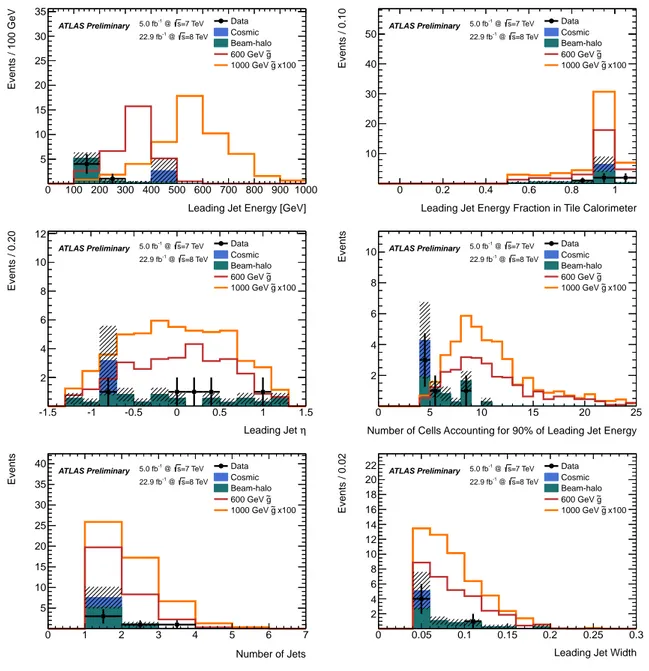
Figure 2: The event yields in the signal region for candidates with all selections (in Table 3) including

the muon segment veto, but excluding jet energy > 100 GeV. All samples are scaled to represent their

anticipated yield in the search region. The hashed band shows the total statistical uncertainty on the

background estimate.

Leading Jet Energy [GeV]

0 100 200 300 400 500 600 700 800 900 1000

Events / 100 GeV

5 10 15 20 25 30 35

Data Cosmic Beam-halo

~g 600 GeV

x100 g~ 1000 GeV ATLAS Preliminary 5.0 fb^-1 @ s=7 TeV

=8 TeV s

-1 @ 22.9 fb

Leading Jet Energy Fraction in Tile Calorimeter

0 0.2 0.4 0.6 0.8 1

Events / 0.10

10 20 30 40 50

Data Cosmic Beam-halo

g~ 600 GeV

x100

~g 1000 GeV ATLAS Preliminary 5.0 fb^-1 @ s=7 TeV

=8 TeV s

-1 @ 22.9 fb

η Leading Jet

-1.5 -1 -0.5 0 0.5 1 1.5

Events / 0.20

2 4 6 8 10 12

Data Cosmic Beam-halo

~g 600 GeV

x100 g~ 1000 GeV ATLAS Preliminary 5.0 fb^-1 @ s=7 TeV

=8 TeV s

-1 @ 22.9 fb

Number of Cells Accounting for 90% of Leading Jet Energy

0 5 10 15 20 25

Events

2 4 6 8

10 ^Data_Cosmic

Beam-halo g~ 600 GeV

x100

~g 1000 GeV ATLAS Preliminary 5.0 fb^-1 @ s=7 TeV

=8 TeV s

-1 @ 22.9 fb

Number of Jets

0 1 2 3 4 5 6 7

Events

5 10 15 20 25 30 35

40 Data

Cosmic Beam-halo

~g 600 GeV

x100 g~ 1000 GeV ATLAS Preliminary 5.0 fb^-1 @ s=7 TeV

=8 TeV s

-1 @ 22.9 fb

Leading Jet Width

0 0.05 0.1 0.15 0.2 0.25 0.3

Events / 0.02

2 4 6 8 10 12 14 16 18 20

22 Data

Cosmic Beam-halo

g~ 600 GeV

x100

~g 1000 GeV ATLAS Preliminary 5.0 fb^-1 @ s=7 TeV

=8 TeV s

-1 @ 22.9 fb

Figure 3: The event yields in the signal region for candidates with all selections (in Table 3) except jet

energy > 300 GeV. All samples are scaled to represent their anticipated yield in the search region. The

hashed band shows the total statistical uncertainty on the background estimate.

examine events from the empty random trigger data in 2011 and 2012 as a function of run number, since the e ff ect can depend strongly on beam conditions. The rate of these events which have a muon segment from noise or other background is calculated. The e ffi ciency per run is applied on a live-time weighted basis to the cosmic background estimate and varies from 98% at the start of 2011 to 70% at the end of 2012. It is also applied to the cosmic background estimate after the muon veto, since the probability to have the cosmic background event pass selections and contribute to the signal region events will depend on it passing the muon veto. The beam-halo background estimate already implicitly accounts for this e ff ect across run periods. For signal, this e ff ect is accounted for inside the timing acceptance calculation, on a per-run basis.

9.2 Timing Acceptance

The expected signal decay rate does not scale with instantaneous luminosity. Rather, at any moment in time, the decay rate is a function of the hypothetical gluino lifetime and the entire history of delivered luminosity. For example, the decay rate anticipated in today’s run is boosted by luminosity delivered yesterday for longer gluino lifetimes. To address the complicated time behavior of the gluino decays, a timing acceptance is defined for each gluino lifetime hypothesis, ϵ

( τ ), as the number of gluinos decaying in an empty bunch crossing divided by the total number that stopped. This means the number of gluinos expected to be reconstructed is L × σ × ϵ

× ϵ

× ϵ

(τ), where L is the integrated luminosity, σ is the gluino cross section weighted by integrated luminosity at 7 and 8 TeV, ϵ

is the stopping fraction, and ϵ

is the reconstruction e ffi ciency.

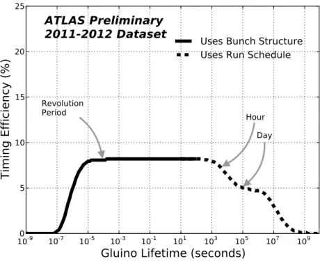
To calculate the timing acceptance for the actual 2011 and 2012 LHC and ATLAS run schedule, measurements are combined of the delivered luminosity in each bunch crossing, the bunch structure of each LHC store, and the live time recorded in empty bunch crossings during each store, all kept in the ATLAS online conditions database. The efficiency calculation is split into short and long gluino lifetimes, to simplify the calculation. For gluino lifetimes less than one second the bunch structure is taken into account, but not the possibility that a gluino produced in one run could decay in a later one. For longer gluino lifetimes the bunch structure is averaged over, but the chance that stopped gluinos from one run decay in a later one is considered. The resulting timing acceptance is presented in Figure 4.

10 Systematic uncertainties

Three sources of systematic uncertainty on the signal efficiency are studied: the R-hadron interaction with matter, the out-of-time decays in the calorimeters, and the e ff ect of the selection criteria. The total uncertainties, added in quadrature, are shown in Table 2. In addition to these, a 3 . 4% uncertainty is assigned on the luminosity measurement [51], correlated for both 2011 and 2012. To account for occasional dead-time due to high trigger rates, a 5% uncertainty was assigned to the timing acceptance;

this accounts for any mismodeling of the accidental muon veto as well. The gluino pair-production cross section uncertainty is not included as a systematic uncertainty but is used when extracting a limit on gluino mass.

10.1 R-hadron-Matter Interactions

The di ff erent signal MC samples are used to estimate the systematic uncertainty on the stopping fraction

due to the scattering model. There are two sources of theoretical uncertainty, the spectrum of R-hadrons

and nuclear interactions. To estimate the e ff ect from di ff erent R-hadron allowed states, three di ff erent

scattering models are employed: generic, Regge and intermediate (see Section 5). Each allows a dif-

10

10

10

10

10

10

10

10

10

10

Gluino Lifetime (seconds)

0 5 10 15 20 25

Timing Efficiency (%)

Revolution

Period Hour

Day

ATLAS Preliminary

2011-2012 Dataset Uses Bunch Structure Uses Run Schedule

Figure 4: The timing acceptance for signal as a function of gluino lifetime (in seconds). This corresponds to the ϵ

( τ ) variable described in the text.

There is also uncertainty from the modeling of nuclear interactions of the R-hadron with the calorimeter since these can a ff ect the stopping fraction. The e ff ect is estimated by calculating the stopping fraction after varying the nuclear cross section up and down by a factor of two. The difference gave a relative uncertainty of 11% which is used as the systematic uncertainty in limit setting.

10.2 Timing in the Calorimeters

Since the R-hadron decay is not synchronized with a bunch crossing it is possible that the calorimeters respond di ff erently to the energy deposits in the simulated signals than in data. The simulation only considers a single bunch crossing for each event; it does not simulate the trigger in multiple bunch crossings and the firing of the trigger for the first bunch crossing which passes the trigger. In reality, a decay at -15 ns relative to a given bunch crossing might fire the trigger for that bunch crossing, or it may fire the trigger for the following bunch crossing. The reconstructed energy response of the calorimeter can vary between these two cases by up to 10% since the reconstruction is optimized for in-time energy deposits. To estimate the systematic uncertainty, the total number of simulated signal events passing the offline selections is studied when varying the timing offset by 5 ns in each direction (keeping the 25 ns range). This variation conservatively covers the timing di ff erence observed between simulated signal jets and cosmic ray muon showers. The minimum and maximum e ffi ciency for each mass point is calculated, and the difference is used as the uncertainty, which is always less than 3% across all mass points.

10.3 Selection Criteria

The systematic uncertainty of selection criteria on signal efficiency was evaluated by varying each se-

lection up and down by its known uncertainty. The uncertainties from each selection are combined in

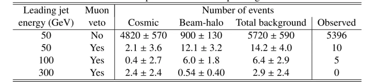
Table 5: The number of observed and expected events corresponding to each of the selection criteria.

Leading jet Muon Number of events

energy (GeV) veto Cosmic Beam-halo Total background Observed

50 No 4820 ± 570 900 ± 130 5720 ± 590 5396

50 Yes 2.1 ± 3.6 12.1 ± 3.2 14.2 ± 4.0 10

100 Yes 0.4 ± 2.7 6.0 ± 1.8 6.4 ± 2.9 5

300 Yes 2.4 ± 2.4 0.54 ± 0.40 2.9 ± 2.4 0

quadrature and are shown in Table 2. Varying only the jet energy scale produces most of the total un- certainty from the selection criteria. The jet energy scale uncertainty is taken to be ±10% to allow for non-pointing R-hadron decays and is significantly larger than is used in standard ATLAS analyses. Al- though test-beam studies showed agreement of energy response between data and simulation for hadronic showers to within a few percent [34], even for non-projective showers, a larger uncertainty is conserva- tively used to cover possible di ff erences between single pions and full jets and between the test-beam detectors studied and the final ATLAS calorimeter.

10.4 Systematic Uncertainties on Background Yield

The systematic uncertainty on the estimated cosmic background arises from the limited statistics of events in the cosmic background region. This statistical uncertainty is scaled by the same factor used to propagate the cosmic background region data yield into expectations of background events in the search regions. Similarly, for the beam-halo background, a systematic uncertainty is assigned based on the statistical uncertainty of the estimates in the search regions.

11 Results

The predicted number of background events agrees well with the observed number of events in the search region. Using these yields, upper limits on the gluino pair production are calculated with a simple event- counting method and then interpret these limits as a function of gluino mass for a given range of gluino lifetimes.

11.1 Limit Setting Procedure

A Bayesian method is used to set 95% credibility level upper limits on the number of signal events that could have been produced. For each limit extraction, pseudo-experiments are run in which the number of observed events is sampled from a Poisson distribution, with mean equal to the expected background, convolved with a Gaussian distribution accounting for systematic uncertainties [52]. A flat prior on signal strength is used, to be consistent with previous results. A Poisson prior gives less conservative limits which are within 10% of those from the flat prior. Since little background is expected and no pseudo-experiment may produce fewer than zero observed events, the distribution of upper limits is bounded from below at − 1 . 15 σ . The input factors to the limit setting algorithm can be seen in Table 5.

The leading jet energy > 300 GeV region is used, except for the more compressed m

−m

models, where

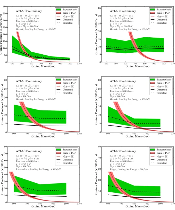
the leading jet energy > 100 GeV region is used. Figure 5 shows the limits on the number of produced

signal events for the various signal models considered, for gluino lifetimes in the plateau acceptance

region between 10

and 10

seconds.

Figure 5: Bayesian upper limits on gluino production versus gluino mass for the various signal models

considered, with gluino lifetimes in the plateau acceptance region between 10

and 10

seconds.

Table 6: Bayesian lower limits on gluino mass for the various signal models considered, with gluino lifetimes in the plateau acceptance region between 10

and 10

seconds.

Leading jet R-hadron Gluino Neutralino Limits on m

(GeV) energy (GeV) model decay mass (GeV) Expected Observed

100 Generic g/q q ¯ + χ ˜

M

− 100 549 572

100 Generic t t ¯ + χ ˜

M

− 380 711 723

300 Generic t t ¯ + χ ˜

100 722 809

300 Generic g/q q ¯ + χ ˜

100 763 857

300 Intermediate g/ q q ¯ + χ ˜

100 635 722

300 Regge g/ q q ¯ + χ ˜

100 687 788

11.2 Results as a Function of Gluino Mass

To provide limits in terms of the gluino mass, m

, we use the gluino pair production cross sections as given by NLL-fast [53, 54]. The number of expected signal events is given by the signal cross sections at 7 and 8 TeV, weighted by the integrated luminosities in the 2011 and 2012 data. The gluino mass limit for each of the signal models, for gluino lifetimes in the plateau acceptance region between 10

and 10

seconds, can be seen in Table 6. Figure 6 shows the mass limits for a particular signal model as a function of the gluino lifetime, for both signal regions.

(a) Leading Jet Energy>100 GeV (b) Leading Jet Energy>300 GeV

Figure 6: Bayesian lower limits on gluino mass versus gluino lifetime, for the two signal regions. An 800 GeV gluino in the generic R-hadron model decaying to g or q q ¯ and a 100 GeV ˜ χ

is used as a reference for the stopping fraction and reconstruction e ffi ciency.

12 Summary

An updated search is presented using 2011 and 2012 data from the ATLAS experiment for stopped long-

lived gluino R-hadrons decaying in the calorimeter, using a jet trigger operating in the empty bunch

from backgrounds, predominantly cosmic ray and beam-halo muons where no muon segment was iden- tified. Limits are set on the gluino mass, for di ff erent gluino decays, gluino lifetimes, and neutralino masses. With a neutralino of mass 100 GeV, the analysis excludes m

< 857 GeV (763 GeV expected), for a gluino lifetime between 10 µs and 1000 s in the generic R-hadron model with equal decays to q q ¯ χ ˜

and g χ ˜

.

References

[1] M. Fairbairn et al., Stable massive particles at colliders, Phys. Rept. 438 (2007) 1–63, arXiv:hep-ph/0611040.

[2] H. Miyazawa, Baryon Number Changing Currents, Prog. Theor. Phys. 36 (6) (1966) 1266–1276.

[3] P. Ramond, Dual Theory for Free Fermions, Phys. Rev. D3 (1971) 2415–2418.

[4] Y. A. Gol’fand and E. P. Likhtman, Extension of the Algebra of Poincare Group Generators and Violation of p Invariance, JETP Lett. 13 (1971) 323–326. [Pisma

Zh.Eksp.Teor.Fiz.13:452-455,1971].

[5] A. Neveu and J. H. Schwarz, Factorizable dual model of pions, Nucl. Phys. B31 (1971) 86–112.

[6] A. Neveu and J. H. Schwarz, Quark Model of Dual Pions, Phys. Rev. D4 (1971) 1109–1111.

[7] J. Gervais and B. Sakita, Field theory interpretation of supergauges in dual models, Nucl. Phys.

B34 (1971) 632–639.

[8] D. V. Volkov and V. P. Akulov, Is the Neutrino a Goldstone Particle?, Phys. Lett. B46 (1973) 109–110.

[9] J. Wess and B. Zumino, A Lagrangian Model Invariant Under Supergauge Transformations, Phys.

Lett. B49 (1974) 52.

[10] J. Wess and B. Zumino, Supergauge Transformations in Four-Dimensions, Nucl. Phys. B70 (1974) 39–50.

[11] N. Arkani-Hamed and S. Dimopoulos, Supersymmetric unification without low energy supersymmetry and signatures for fine-tuning at the LHC, JHEP 06 (2005) 073.

[12] N. Arkani-Hamed, S. Dimopoulos, G. F. Giudice, and A. Romanino, Aspects of split supersymmetry, Nucl. Phys. B 709 (2005) 3–46.

[13] M. Dine and W. Fischler, A Phenomenological Model of Particle Physics Based on Supersymmetry, Phys. Lett. B110 (1982) 227.

[14] L. Alvarez-Gaume, M. Claudson, and M. B. Wise, Low-Energy Supersymmetry, Nucl. Phys. B207 (1982) 96.

[15] C. R. Nappi and B. A. Ovrut, Supersymmetric Extension of the SU(3) x SU(2) x U(1) Model, Phys.

Lett. B113 (1982) 175.

[16] M. Dine and A. E. Nelson, Dynamical supersymmetry breaking at low-energies, Phys. Rev. D48

(1993) 1277–1287, arXiv:hep-ph/9303230.

[17] M. Dine, A. E. Nelson, and Y. Shirman, Low-energy dynamical supersymmetry breaking simplified, Phys. Rev. D51 (1995) 1362–1370, arXiv:hep-ph/9408384.

[18] M. Dine, A. E. Nelson, Y. Nir, and Y. Shirman, New tools for low-energy dynamical supersymmetry breaking, Phys. Rev. D53 (1996) 2658–2669, arXiv:hep-ph/9507378.

[19] S. Raby, Gauge-mediated SUSY breaking at an intermediate scale, Phys. Rev. D 56 (1997) 2852.

[20] T. Appelquist, H. Cheng, and B. A. Dobrescu, Bounds on universal extra dimensions, Phys. Rev.

D 64 (2001) .

[21] C. Friberg, E. Norrbin, and T. Sjostrand, QCD aspects of leptoquark production at HERA, Phys.

Lett. B. 403 (1997) 329.

[22] M. Johansen, J. Edsjo, S. Hellman, and D. Milstead, Long-lived stops in MSSM scenarios with a neutralino LSP, JHEP 1008 (2010) 005, arXiv:1003.4540 [hep-ph].

[23] J. A. Evans and Y. Kats, LHC Coverage of RPV MSSM with Light Stops, JHEP 1304 (2013) 028, arXiv:1209.0764 [hep-ph].

[24] A. C. Kraan, Interactions of heavy stable hadronizing particles, Eur. Phys. J. C37 (2004) 91–104, arXiv:hep-ex/0404001.

[25] L. Evans and P. Bryant, LHC Machine, JINST 3 (2008) S08001.

[26] V. M. Abazov √ et al. [D0 Collaboration], Search for stopped gluinos from p p collisions at ¯ s = 1.96 TeV, Phys. Rev. Lett. 99 (2007) 131801.

[27] CMS Collaboration, Search for stopped gluinos in pp collisions at √

s = 7 TeV , Phys. Rev. Lett.

106 (2011) 011801, arXiv:hep-ex/1011.5861.

[28] CMS Collaboration, Search for stopped long-lived particles produced in pp collisions at √ s = 7 TeV, JHEP 1208 (2012) 026, arXiv:1207.0106 [hep-ex].

[29] ATLAS Collaboration, Search for decays of stopped, long-lived particles from 7 TeV pp collisions with the ATLAS detector, Eur.Phys.J. C72 (2012) 1965, arXiv:1201.5595 [hep-ex].

[30] ATLAS Collaboration, Search for stable hadronising squarks and gluinos with the ATLAS experiment at the LHC, Phys. Lett. B701 (2011) 1–19, arXiv:hep-ex/1103.1984.

[31] ATLAS Collaboration, Search for heavy long-lived charged particles with the ATLAS detector in pp Collisions at √

s = 7 TeV , Phys. Lett. B703 (2011) 428–446, arXiv:hep-ex/1106.4495.

[32] ATLAS Collaboration, The ATLAS Experiment at the CERN Large Hadron Collider, JINST 3 (2008) S08003.

[33] M. Cacciari, G. P. Salam, and G. Soyez, The anti-k

jet clustering algorithm, JHEP 04 (2008) 063.

[34] A. Dotti, A. Lupi, and C. Roda, Results from ATLAS Tile Calorimeter: a comparison between data and Geant4 simulation, Nuclear Physics B - Proceedings Supplements 150 (2006) no. 0, 106 – 109.

[35] ATLAS Collaboration, Measurement of inclusive jet and dijet cross sections in proton-proton

[36] E. Gianfelice-Wendt, W. Bartmann, A. Boccardi, C. Bracco, E. Bravin, et al., LHC Abort Gap Cleaning Studies During Luminosity Operation, FERMILAB-CONF-12-142-APC, Fermilab, 2012.

[37] ATLAS Collaboration, Measurement of the Rate of Collisions from Satellite Bunches for the April-May 2010 LHC Luminosity Calibration, ATLAS-CONF-2010-102, CERN, Geneva, Dec, 2010.

[38] C. Ohm and T. Pauly, The ATLAS beam pick-up based timing system, Nucl.Instrum.Meth. A623 (2010) 558–560, arXiv:0905.3648 [physics.ins-det].

[39] ATLAS Collaboration, Performance of the ATLAS Trigger System in 2010, arXiv:hep-ex/1110.1530v1.

[40] T. Sjostrand, S. Mrenna, and P. Skands, PYTHIA 6.4 Physics and Manual, JHEP 05 (2006) 026, arXiv:hep-ph/0603175.

[41] B. Andersson, G. Gustafson, G. Ingelman, and T. Sjostrand, Parton Fragmentation and String Dynamics, Phys. Rept. 97 (1983) 31–145.

[42] GEANT4 Collaboration, GEANT4: A simulation toolkit, Nucl. Instrum. Meth. A506 (2003) 250–303.

[43] ATLAS Collaboration, The ATLAS simulation infrastructure, Eur. Phys. J. C70 (2010) 823–874, arXiv:hep-ex/1005.4568v1.

[44] R. Mackeprang and A. Rizzi, Interactions of coloured heavy stable particles in matter, Eur. Phys.

J. C50 (2007) 353–362, arXiv:hep-ph/0612161.

[45] Y. R. de Boer, A. B. Kaidalov, D. A. Milstead, and O. I. Piskounova, Interactions of Heavy Hadrons using Regge Phenomenology and the Quark Gluon String Model, J. Phys. G35 (2008) 075009, arXiv:hep-ex/0710.3930.

[46] R. Mackeprang and D. Milstead, An Updated Description of Heavy-Hadron Interactions, Eur.

Phys. J. C66 (2010) 493–501, arXiv:hep-ph/0908.1868.

[47] G. Farrar, R. Mackeprang, D. Milstead, and J. Roberts, Limit on the mass of a long-lived or stable gluino, arXiv:1011.2964.

[48] A. Arvanitaki, S. Dimopoulos, A. Pierce, S. Rajendran, and J. G. Wacker, Stopping gluinos, Phys.

Rev. D76 (2007) 055007, arXiv:hep-ph/0506242.

[49] L. S. Azhgirey, I. S. Baishev, K. M. Potter, and V. Talanov, Machine Induced Background in the High Luminosity Experimental Insertion of the LHC Project, CERN-LHC-Project-Report-722.

[50] ATLAS Collaboration, Characterisation and mitigation of beam-induced backgrounds observed in the ATLAS detector during the 2011 proton-proton run, arXiv:1303.0223 [hep-ex].

[51] ATLAS Collaboration, Luminosity Determination in pp Collisions at √

s = 7 TeV Using the ATLAS Detector at the LHC, Eur.Phys.J. C71 (2011) 1630, arXiv:1101.2185 [hep-ex].

[52] J. Heinrich, C. Blocker, J. Conway, L. Demortier, L. Lyons, G. Punzi, and P. K. Sinervo, Interval estimation in the presence of nuisance parameters. 1. Bayesian approach,

arXiv:physics/0409129.

[53] LHC SUSY Cross Section Working Group, SUSY cross sections for 7 and 8 TeV , https: // twiki.cern.ch / twiki / bin / view / LHCPhysics / SUSYCrossSections.

[54] W. Beenakker, S. Brensing, M. Kramer, A. Kulesza, E. Laenen, et al., Squark and Gluino Hadroproduction, Int.J.Mod.Phys. A26 (2011) 2637–2664, arXiv:1105.1110 [hep-ph].

A Additional material for approval

Figure 7: Left: A beam-halo candidate event during an unpaired bunch crossing in data. This event

passed all the selection criteria except for the muon segment veto. Right: A cosmic ray muon candidate

event during an empty bunch crossing in data. This event passed all the selection criteria except for

the muon segment veto. In both plots, white squares filled with red squares show reconstructed energy

deposits in TileCal cells above noise threshold (the fraction of red area indicates the amount of energy

in the cell), purple bars show a histogram of total energy in projective TileCal towers, jets are shown by

open red trapezoids, muon segments by green line segments in each muon station, and muon tracks by

continuous thin yellow lines.

Figure 8: Event display showing several TileCal cells overlaid with particle steps from the Geant4 sim- ulation of an R-hadron decay to a jet and a neutralino. Charged particles are green, photons are blue, and other neutral particles (including neutrons) are red. White squares filled with red squares show re- constructed energy deposits in TileCal cells above noise threshold (the fraction of red area indicates the amount of energy in the cell), purple bars show a histogram of total energy in projective TileCal towers, and jets are shown by open red trapezoids.

Table 7: Cut Flow Table for signal samples with ˜ g → g/qq χ ˜

decays. The cumulative efficiency is pro- vided for each successive selection. The samples correspond to the generic R-hadron model as described in Section 5. The gluino mass is varied with a fixed neutralino mass of 100 GeV used in all cases. The quoted uncertainties are statistical only.

Signal MC samples: gluino masses with m

= 100 GeV

Selection criteria 400 GeV 600 GeV 800 GeV 1000 GeV

Trigger 63.09 ± 0.71 % 69.10 ± 0.70 % 71.13 ± 0.70 % 73.48 ± 0.71 %

Leading jet |η| < 1.2 55.75 ± 0.73 % 59.69 ± 0.74 % 60.52 ± 0.75 % 62.82 ± 0.78 %

N jets < 6 55.75 ± 0.73 % 59.65 ± 0.74 % 60.40 ± 0.75 % 62.62 ± 0.78 %

Fractional E

> 0.5 55.75 ± 0.73 % 59.60 ± 0.74 % 60.23 ± 0.75 % 62.38 ± 0.78 %

Leading jet n90 > 3 49.09 ± 0.73 % 53.59 ± 0.75 % 54.15 ± 0.77 % 56.77 ± 0.79 %

Leading jet width > 0.04 23.48 ± 0.62 % 27.36 ± 0.67 % 29.91 ± 0.71 % 31.18 ± 0.74 %

Leading jet tile E frac. > 0.5 16.99 ± 0.55 % 19.84 ± 0.60 % 22.34 ± 0.64 % 23.04 ± 0.68 %

Leading jet energy > 50 GeV 16.99 ± 0.55 % 19.84 ± 0.60 % 22.34 ± 0.64 % 23.04 ± 0.68 %

Muon segment veto 14.49 ± 0.51 % 15.08 ± 0.54 % 15.48 ± 0.56 % 14.75 ± 0.57 %

Leading jet energy > 100 GeV 14.06 ± 0.51 % 15.01 ± 0.54 % 15.46 ± 0.56 % 14.75 ± 0.57 %

Leading jet energy > 300 GeV 0.47 ± 0.10 % 10.61 ± 0.46 % 13.94 ± 0.53 % 14.08 ± 0.56 %

Figure 9: Some candidate event displays from 2011 (top) and 2012 (bottom) data passing all selec-

tions. White squares filled with red squares show reconstructed energy deposits in TileCal cells above

noise threshold (the fraction of red area indicates the amount of energy in the cell), purple bars show

a histogram of total energy in projective TileCal towers, and jets are shown by red semi-transparent

trapezoids. Muons segments are drawn but none are reconstructed in these events.