, on behalf of the ATLAS collaboration

c Owned by the authors, published by EDP Sciences, 2017

Searches for direct pair production of third generation squarks with the ATLAS detector

Nicolas Köhler

, on behalf of the ATLAS collaboration

1

Max Planck Institute for Physics, Föhringer Ring 6, 80805 Munich, Germany

Abstract. Naturalness arguments for weak-scale supersymmetry favour supersymmetric partners of the third generation quarks with masses not too far from those of their Stan- dard Model counterparts. Top or bottom squarks with masses less than or around one TeV can also give rise to direct pair production rates at the Large Hadron Collider (LHC) that can be observed in the data sample recorded by the ATLAS detector. This document presents recent ATLAS results from searches for direct top and bottom squark pair pro- duction considering both R-parity conserving and R-parity violating scenarios, using the data collected during the LHC Run 2 at a centre-of-mass energy of √ s = 13 TeV.

1 Introduction

Supersymmetry (SUSY) [1] is one of the most attractive extensions of the Standard Model (SM) of particle physics. It can resolve the gauge hierarchy problem [2–5] by introducing supersymmetric partners of the known bosons and fermions and extending the Higgs boson sector to 5 Higgs bosons, whose superpartners mix together with the electroweak gauginos to the neutralinos and charginos.

Since the supersymmetric Langrangian contains terms which can violate the baryon and lepton number which allows for rapid proton decay, often R-parity conservation (RPC) is introduced which results in the lightest supersymmetric particle (LSP) being stable and thus, in case the LSP is the lightest neutralino, to an ideal dark matter candidate [6, 7]. If R-parity is violated, this for example can nicely explain the baryon-lepton-asymmetry or the masses of neutrinos [8–10].

Naturalness arguments favour the third-generation squarks to be the lightest colored supersym- metric particles [11, 12], i.e. their masses should be in the TeV range and thus, directly accessible at the Large Hadron Collider (LHC) at CERN. This document summarizes the ATLAS [13] search program for third-generation squarks performed during LHC Run 2 at a centre-of-mass energy of

√ s = 13 TeV. The datasets used by the analyses mentioned in this document comprise an integrated luminosity of 36.1 fb

and 36.7 fb

from 2015 and 2016 depending on the data quality requirements.

2 Summary of the searches

2.1 R-parity conserving scenarios

Assuming R-parity conservation, supersymmetric particles are produced in pairs and the LSP is stable.

Since it escapes the detector without any interaction, signatures with large missing tranverse momen-

ae-mail: nicolas.koehler@cern.ch

2

tum E

are expected. Figure 1 shows the mass spectrum of the different SUSY scenarios depending on the particle nature of the LSP. For a bino-like neutralino ˜ χ

as the LSP, there are 3 different decay scenarios for the top squark ˜ t

(cf. Figure 2). For m

< m

+ m

, where m

is the mass of the ˜ t

, m

is the mass of the W boson and m

is the mass of the ˜ χ

, either a 4-body decay into a b-quark jet, two distinct fermions f and f

and a neutralino or a flavour-changing neutral current (FCNC) process with a charm quark (˜ t

→ c χ ˜

) occurs, which is targeted by the 1- and 2-lepton final state analyses. For higher m

< m

, where m

is the mass of the top quark, a 3-body decay into a b-quark jet, a W boson and a neutralino occurs targeted by all, 0-/1- and 2-lepton final state analyses, the same for m

> m

, where a 2-body decays into a top quark and a neutralino (˜ t

→ t + χ ˜

) happens [14].

˜t1,˜b1,˜⁰₁,˜^±1,˜⁰₂,˜⁰₃

˜t1,˜b1,˜⁰₁,˜^±1,˜⁰₂,˜⁰₃

˜t1,˜b1,˜⁰₁,˜^±1,˜⁰₂,˜⁰₃

˜t1,˜b1,˜⁰₁,˜^±1,˜⁰₂,˜⁰₃ t˜1,˜b1,˜⁰₁,˜^±1,˜⁰₂,˜⁰₃

˜t1,˜b1,˜⁰1,˜^±1,˜⁰2,˜⁰3 ˜t1,˜b1,˜⁰₁,˜^±₁,˜⁰₂,˜⁰₃ t˜1,˜b1,˜⁰₁,˜^±₁,˜⁰₂,˜⁰₃

˜t1,˜b1,˜⁰₁,˜^±₁,˜⁰₂,˜⁰₃ ˜t1,(˜b1)

a) pure bino LSP b) wino NLSP c) higgsino LSP d) bino/higgsino mixa) pure bino LSP b) wino NLSP c) higgsino LSP d) bino/higgsino mixa) pure bino LSP b) wino NLSP c) higgsino LSP d) bino/higgsino mixa) pure bino LSP b) wino NLSP c) higgsino LSP d) bino/higgsino mix

sparticlemasses

Figure 1: Illustration of the sparticle mass spectrum for various LSP scenarios: a) Pure bino LSP, b) wino next-to-lightest supersymmetric particle (NLSP), c) higgsino LSP, and d) bino / higgsino mix.

The ˜ t

and ˜ b

decay into di ff erent electroweakino states in the scenarios: the bino state (red lines), the wino states (blue lines), or the higgsino states (green lines), with possibly the subsequent decays into the LSP [14].

˜t¹!bff⁰˜⁰¹

˜t¹!bW

˜⁰¹

˜t¹!t˜⁰¹ m>0

m>m^˜t1 m>m^W

+m^b m>0

m>m^˜t1 m>m^W

+m^b

m >0 m > m˜t1

m > m_W+m_b m=m˜t1 m_˜0 1

0 100 200 300

0 100 200 300 0 100 200 3000 100 200 300

01002003000100200300

˜t¹!c˜⁰¹

m>m^t m˜t1< m_˜0

1

m˜¹₀[GeV] m˜t1[GeV]

m^˜t1[GeV]m˜

0 1

[GeV]

Figure 2: Illustration of the preferred top squark decay modes in the plane of the ˜ t

and ˜ χ

mass, where the latter is assumed to be the lightest supersymmetric particle. Top squark decays to supersymmetric particles other than the LSP are not displayed [14].

2.1.1 Final states with no leptons

If the top quark from the ˜ t

→ t + χ ˜

decay decays fully hadronically, there are no leptons in the final

state and the E

is originating only from the ˜ χ

. Figure 3a shows the masses of the leading and

tum E

are expected. Figure 1 shows the mass spectrum of the different SUSY scenarios depending on the particle nature of the LSP. For a bino-like neutralino ˜ χ

as the LSP, there are 3 different decay scenarios for the top squark ˜ t

(cf. Figure 2). For m

< m

+ m

, where m

is the mass of the ˜ t

, m

is the mass of the W boson and m

is the mass of the ˜ χ

, either a 4-body decay into a b-quark jet, two distinct fermions f and f

and a neutralino or a flavour-changing neutral current (FCNC) process with a charm quark (˜ t

→ c χ ˜

) occurs, which is targeted by the 1- and 2-lepton final state analyses. For higher m

< m

, where m

is the mass of the top quark, a 3-body decay into a b-quark jet, a W boson and a neutralino occurs targeted by all, 0-/1- and 2-lepton final state analyses, the same for m

> m

, where a 2-body decays into a top quark and a neutralino (˜ t

→ t + χ ˜

) happens [14].

˜t1,˜b1,˜⁰₁,˜^±1,˜⁰₂,˜⁰₃

˜t1,˜b1,˜⁰₁,˜^±1,˜⁰₂,˜⁰₃

˜t1,˜b1,˜⁰₁,˜^±1,˜⁰₂,˜⁰₃

˜t1,˜b1,˜⁰₁,˜^±1,˜⁰₂,˜⁰₃ ˜t1,˜b1,˜⁰₁,˜^±1,˜⁰₂,˜⁰₃

˜t1,˜b1,˜⁰1,˜^±1,˜⁰2,˜⁰3 ˜t1,˜b1,˜⁰₁,˜^±₁,˜⁰₂,˜⁰₃

˜t1,˜b1,˜⁰₁,˜^±₁,˜⁰₂,˜⁰₃

˜t1,˜b1,˜⁰₁,˜^±₁,˜⁰₂,˜⁰₃ t˜1,(˜b1)

a) pure bino LSP b) wino NLSP c) higgsino LSP d) bino/higgsino mixa) pure bino LSP b) wino NLSP c) higgsino LSP d) bino/higgsino mixa) pure bino LSP b) wino NLSP c) higgsino LSP d) bino/higgsino mixa) pure bino LSP b) wino NLSP c) higgsino LSP d) bino/higgsino mix

sparticlemasses

Figure 1: Illustration of the sparticle mass spectrum for various LSP scenarios: a) Pure bino LSP, b) wino next-to-lightest supersymmetric particle (NLSP), c) higgsino LSP, and d) bino / higgsino mix.

The ˜ t

and ˜ b

decay into di ff erent electroweakino states in the scenarios: the bino state (red lines), the wino states (blue lines), or the higgsino states (green lines), with possibly the subsequent decays into the LSP [14].

˜t¹!bff⁰˜⁰¹

˜t¹!bW

˜⁰¹

˜t¹!t˜⁰¹ m>0

m>m^˜t1 m>m^W

+m^b m>0

m>m^˜t1 m>m^W

+m^b

m >0 m > m˜t1

m > m_W+m_b m=m˜t1 m_˜0 1

0 100 200 300

0 100 200 300 0 100 200 3000 100 200 300

01002003000100200300

˜t¹!c˜⁰¹

m>m^t m˜t1< m_˜0

1

m˜¹₀[GeV] m˜t1[GeV]

m˜t1[GeV]m˜

0 1

[GeV]

Figure 2: Illustration of the preferred top squark decay modes in the plane of the ˜ t

and ˜ χ

mass, where the latter is assumed to be the lightest supersymmetric particle. Top squark decays to supersymmetric particles other than the LSP are not displayed [14].

2.1.1 Final states with no leptons

If the top quark from the ˜ t

→ t + χ ˜

decay decays fully hadronically, there are no leptons in the final state and the E

is originating only from the ˜ χ

. Figure 3a shows the masses of the leading and

subleading reclustered radius R =

η

+ φ

= 1.2 jets for a simulated ˜ t

→ t + χ ˜

scenario. The peaks around m

and m

allow for a good discrimination against all SM backgrounds not containing 2 top quarks (TT), 1 top quark and 1 W boson (TW) or at least 1 top quark (T0) [15]. Another very useful variable is the transverse mass between the b-quark jet closest to E

and E

itself, which is called m

(cf. Figure 3b). For top quark pair production (t t), it has a kinematic endpoint at ¯ m

, which allows for a good t t ¯ suppression.

[GeV]

0 R=1.2

mjet,

200 400 600 800

[GeV]1 =1.2Rjet,m

0 200 400 600 800

Fraction of events

0.00 0.02 0.04

ATLAS

Simulation = 13 TeV s

) = (1000,1) GeV χ∼0₁

, t~1

( TT

TWT0

(a) Illustration of the different signal-regions (TT, TW, and T0) in the R = 1.2 reclustered top- candidate mass plane (jet with second highest trans- verse momentum vs. highest one) for simulated di- rect top-squark pair production with (m

, m

1

) = (1000, 1) GeV after the preselection [15].

Events / 50 GeV

0 2000 4000

6000 ^Data

SM Total tt Single Top

+V tt W Z Diboson

)=(600,300) GeV 1 χ0 ,∼ t~1 20 x (

)=(1000,1) GeV 1 χ0 ,∼ t~1 100 x (

ATLAS _-1

=13 TeV, 36.1 fb s m^bT^,min>50 GeV preselection +

[GeV]

,min bT

0 200 400 m600

Data / SM

0.0 0.5 1.0 1.5 2.0

(b) Distribution of m

after the preselection of the 0-lepton final state [15]. The bottom panel shows the ratio of the number of data events to the total SM pre- diction. The hatched band shows the combination of statistical and detector-related systematic uncertain- ties. The rightmost bin contains overflow events.

Figure 3

(a) Illustration of the event hemispheres (ISR and MET= E

) created by the recursive jigsaw algo- rithm [16] out of the centre-of-mass (CM) frame.

Events / 0.1

0 20 40

Data SM Total

tt Single Top

+V tt W Diboson Multijet

)=(400,227) GeV 1 χ0 ,∼ t~1 (

)=(500,327) GeV 1 χ0 ,∼ t~1 (

ATLAS _-1

=13 TeV, 36.1 fb SRC1-5s

RISR

0.2 0.4 0.6 0.8

Data / SM

0.0 0.5 1.0 1.5 2.0

(b) Distribution of R

after the maximum likelihood fit in the SRC1-5 signal region described in [15]. The hatched uncertainty band shows the MC statistical and detector-related systematic uncertainties. In addi- tion, the distribution for a representative signal model is shown.

Figure 4

4 Compressed scenarios (m

− m

1

∼ m

) suffer from low E

which results in final states looking similar to t¯ t. In case of an energetic jet from initial state radiation (ISR), the whole system gets boosted which results in a significant amount of E

. In order to increase the sensitivity in those regions, the so-called recursive jigsaw algorithm [16] is applied. The algorithm maximizes the amount of back- to-back transverse momenta (p

) of all possible hemispheres created by splitting the event by a plane into 2 pieces (cf. Figure 4a). Ideally, after having applied the algorithm, one hemisphere contains the decay products of the top squarks, including the E

, whereas the other one includes the ISR jet and thus, is called ISR system. The ratio of the E

and the p

of the ISR system is called R

and is shown in Figure 4b.

In none of the signal regions any excess above the SM expectation was found, exclusion limits were set combining all 0-lepton signal regions. Figure 5a shows the 95% confidence level exclusion limits. The exclusion shape along the mass diagonal is obtained by the recursive jigsaw algorithm.

Decays of the lighter bottom squark ˜ b

are kinematically very similar to ˜ t

decays which allows to also interpret the 0-lepton selection with few adaptions in scenarios where the ˜ b

decays via ˜ b

→ t+ χ ˜

[17]. The corresponding exclusion limits are shown in Figure 5b.

[GeV]

t~1

200 400 600 800 1000m 1200

[GeV]0 1χ∼m

0 100 200 300 400 500 600 700 800 900

SRA+SRB+SRC+SRD+SRE + m_t ^0∼χ1 < m₁ mt~

0χ1

∼ + m_b W + m < m₁ mt~

) = 100%

0

χ∼1

t(*) 1→ t~

Top squark pair production, B(

=13 TeV, 36.1 fb-1

s

ATLAS Observed limit (±1σ_theory^SUSY) exp) 1σ Expected limit (±

=8 TeV s -1, ATLAS 20 fb Limits at 95% CL

(a) ˜ t

versus ˜ χ

mass plane in the scenario where both top squarks decay via ˜ t

→ t + χ ˜

combining signal regions SRA, SRB, SRC, SRD and SRE described in [15].

[GeV]

b~1

200 400 600 800 1000 m1200

[GeV]0 1χ∼m

0 100 200 300 400 500 600 700 800 900 1000

0

χ∼1

b

1→ b~

Bottom squark pair production,

=13 TeV, 36.1 fb-1

s ATLAS

=8 TeV s -1, + 2 b-jets, 20.1 fb T ATLAS Emiss

=13 TeV s , + 2 b-jets, 3.2 fb-1 T ATLAS Emiss

Best b0L SR

theory) σSUSY

1 Observed limit (±

exp) 1σ Expected limit (±

forbidden

0χ1

b ∼

1→

~b

(b) ˜ b

versus ˜ χ

mass plane in the scenario where both bottom squarks decay via ˜ b

→ t+ χ ˜

and the SR with the best expected sensitivity is adopted for each point of the parameter space as described in [17].

Figure 5: Observed (red) and expected (blue) exclusion contours at 95% CL, as well as ± 1σ variation

of the expected limit. The yellow band around the expected limit shows the impact of the experimental

and SM background theoretical uncertainties. The dotted lines show the impact on the observed limit

of the variation of the nominal signal cross-section by ± 1σ of its theoretical uncertainties. Observed

limits from all third-generation Run-1 searches [18] at √ s = 8 TeV using 20 fb

of data overlaid for

comparison in blue [15, 17].

5 Compressed scenarios (m

− m

1

∼ m

) suffer from low E

which results in final states looking similar to t¯ t. In case of an energetic jet from initial state radiation (ISR), the whole system gets boosted which results in a significant amount of E

. In order to increase the sensitivity in those regions, the so-called recursive jigsaw algorithm [16] is applied. The algorithm maximizes the amount of back- to-back transverse momenta (p

) of all possible hemispheres created by splitting the event by a plane into 2 pieces (cf. Figure 4a). Ideally, after having applied the algorithm, one hemisphere contains the decay products of the top squarks, including the E

, whereas the other one includes the ISR jet and thus, is called ISR system. The ratio of the E

and the p

of the ISR system is called R

and is shown in Figure 4b.

In none of the signal regions any excess above the SM expectation was found, exclusion limits were set combining all 0-lepton signal regions. Figure 5a shows the 95% confidence level exclusion limits. The exclusion shape along the mass diagonal is obtained by the recursive jigsaw algorithm.

Decays of the lighter bottom squark ˜ b

are kinematically very similar to ˜ t

decays which allows to also interpret the 0-lepton selection with few adaptions in scenarios where the ˜ b

decays via ˜ b

→ t+˜ χ

[17]. The corresponding exclusion limits are shown in Figure 5b.

[GeV]

t~1

200 400 600 800 1000m 1200

[GeV]0 1χ∼m

0 100 200 300 400 500 600 700 800 900

SRA+SRB+SRC+SRD+SRE + m_t ^∼0χ1 < m₁ mt~

0χ1

∼ + m_b W + m < m₁ mt~

) = 100%

0

χ∼1

t(*) 1→ t~

Top squark pair production, B(

=13 TeV, 36.1 fb-1

s

ATLAS Observed limit (±1σ_theory^SUSY) exp) 1σ Expected limit (±

=8 TeV s -1, ATLAS 20 fb Limits at 95% CL

(a) ˜ t

versus ˜ χ

mass plane in the scenario where both top squarks decay via ˜ t

→ t + χ ˜

combining signal regions SRA, SRB, SRC, SRD and SRE described in [15].

[GeV]

b~1

200 400 600 800 1000 m1200

[GeV]0 1χ∼m

0 100 200 300 400 500 600 700 800 900 1000

0

χ∼1

b

1→ b~

Bottom squark pair production,

=13 TeV, 36.1 fb-1

s ATLAS

=8 TeV s -1, + 2 b-jets, 20.1 fb T ATLAS Emiss

=13 TeV s , + 2 b-jets, 3.2 fb-1 T ATLAS Emiss

Best b0L SR

theory) σSUSY

1 Observed limit (±

exp) 1σ Expected limit (±

forbidden

01

∼χ

→ b b1

~

(b) ˜ b

versus ˜ χ

mass plane in the scenario where both bottom squarks decay via ˜ b

→ t+ χ ˜

and the SR with the best expected sensitivity is adopted for each point of the parameter space as described in [17].

Figure 5: Observed (red) and expected (blue) exclusion contours at 95% CL, as well as ± 1σ variation of the expected limit. The yellow band around the expected limit shows the impact of the experimental and SM background theoretical uncertainties. The dotted lines show the impact on the observed limit of the variation of the nominal signal cross-section by ± 1σ of its theoretical uncertainties. Observed limits from all third-generation Run-1 searches [18] at √ s = 8 TeV using 20 fb

of data overlaid for comparison in blue [15, 17].

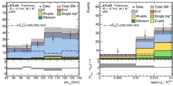
2.1.2 Final states with one lepton

The analysis searching for direct top squark production with one isolated lepton in the final state covers scenarios with 2-, 3- and 4-body ˜ t

decays [14]. For the 2-body decay, besides a high E

, also one hadronically decaying top quark is required. Additional cuts on variables which try to reconstruct the leptonic decay, such as the transverse mass between the lepton and the E

and the asymmetric stransverse mass help to reject the SM backgrounds which are mainly t t ¯ production. While in case of 2-body decay scenarios, a cut&count analysis is used, for the 3- and 4-body decays, kinematic shapes are needed, since the same final-state objects have significanctly lower momenta which are typically still above the reconstruction thresholds. The asymmetric stransverse mass am

shown in Figure 6a) is a powerful discriminant for separating dileptonic t t ¯ (where both W bosons decay leptonically) from signal since it has an kinematic endpoint at m

. For the 4-body decay scenario, a shape-fit in am

is applied whereas for the 3-body decay scenario, a shape-fit of the lepton p

divided by the E

distribution is applied (cf. Figure 6b).

[GeV]

amT2

80 85 90 95 100 105 110 115 120 125 130

totσ) / exp - nobs(n 2−

0 2

Events

0 10 20 30 40 50 60 70

80 Data Total SM

tt tt+V W+jets Single top Diboson

)=(400,250) GeV

1

χ∼0 1, t~

m(

ATLAS Preliminary_-1 = 13 TeV, 36.1 fb bWNs

(a) am

in the 4-body decay scenario signal region bWN as described in [14].

missT T / E lepton p

0 0.005 0.01 0.015 0.02

totσ) / exp - nobs(n 2−

0 2

Events

0 10 20 30 40 50

60 Data Total SM

tt tt+V W+jets Single top Diboson Z+jets )=(350,330) GeV

1

χ∼0 1, t~

m(

ATLAS Preliminary_-1 = 13 TeV, 36.1 fb bffNs

(b) Lepton p

/E

in the 3-body decay scenario sig- nal region bffN as described in [14].

Figure 6: Distributions of kinematic variables used in the shape-fit analyses: The full event selection in the corresponding signal region is applied, except for the requirement that is imposed on the variable being plotted. The predicted SM backgrounds are scaled with the normalisation factors obtained from the corresponding control regions. The hashed area around the total SM prediction includes statistical and experimental uncertainties. The last bin contains overflows. Benchmark signal models are overlaid for comparison. The bottom panels show the difference between data (n

) and the predicted SM background (n

) divided by the total uncertainty (σ

) [14].

As for the 0-lepton final state, the recursive jigsaw algorithm is used for the the compressed region,

but the ISR variables are additionally put into a boosted decision tree [19] in order to increase the

sensitivity since the 1-lepton final state has an additional neutrino which contributes to the E

.

6

EPJ Web of Conferences 182, 02065 (2018) https://doi.org/10.1051/epjconf/201818202065 ICNFP 2017

EPJ Web of Conferences

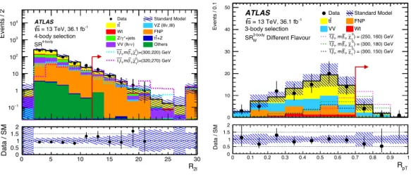
2.1.3 Final states with two leptons

A final state with two leptons has the smallest branching fraction compared to the 0-lepton or 1-lepton final states, but the leptonic top quark decay allows for the best coverage of the 3- and 4-body decay scenarios [20]. For the 4-body decay scenario, where objects with low momenta are expected, an E

trigger is used assuming the presence of an ISR jet. For this region, the ratio between the E

and the p

of the 2-lepton system (R

, cf. Figure 7a) is used as discriminating variable. For the 3-body decay scenario, there are dedicated signal regions for m

− m

being either close to m

or m

. Here, so-called super-razor variables are used, similar to the recursive jigsaw variables in the 0-lepton and 1-lepton final states. Figure 7b shows the ratio between the sum of transverse momenta of the visible particles including the E

and the energy of the razor frame R

, similar to R

mentioned before.

R2l

Events / 2

1

10−

1 10 102

103

104 ATLAS = 13 TeV, 36.1 fb-1

s

4-body

SR4-body selection

Data tt Wt

*+jets Z/γ

) ν VV (llν

Standard Model ,llll) VZ (lllν FNP

+Z tt Others )=(300,220) GeV 1 χ∼0 1, t~

1,m(

1t~

t~

)=(320,270) GeV 1 χ∼0 1, t~

1,m(

1t~

t~

R2l

0 5 10 15 20 25 30

Data / SM 00.511.52

(a) R

applying a 4-body selection as described in [20].

RpT

Events / 0.1

0 10 20 30 40

50 Data Standard Model

tt FNP

VV Wt

ATLAS = 13 TeV, 36.1 fb-1

3-body selections Different Flavour

3-body

SRW t~1t~1, m(t~1,χ∼ ⁰₁) = (250, 160) GeV ) = (300, 180) GeV 0

χ∼1 1, t~

1, m(

1t~

t~

) = (300, 150) GeV 0

χ∼1 1, t~

1, m(

1t~

t~

RpT

0 0.1 0.2 0.3 0.4 0.5 0.6 0.7 0.8 0.9 1

Data / SM

0 0.51 1.52

(b) R

applying a 3-body selection as described in [20].

Figure 7: Distributions of discriminating variables after the background fit in the various signal re-

gions. The contributions from all SM backgrounds are shown as a histogram stack; the hatched bands

represent the total statistical and systematic uncertainty. The rightmost bin of each plot includes over-

flow events. Reference top squark pair production signal models are overlayed for comparison. Red

arrows indicate the signal region selection criteria [20].

EPJ Web of Conferences 182, 02065 (2018) https://doi.org/10.1051/epjconf/201818202065 ICNFP 2017

EPJ Web of Conferences

2.1.3 Final states with two leptons

A final state with two leptons has the smallest branching fraction compared to the 0-lepton or 1-lepton final states, but the leptonic top quark decay allows for the best coverage of the 3- and 4-body decay scenarios [20]. For the 4-body decay scenario, where objects with low momenta are expected, an E

trigger is used assuming the presence of an ISR jet. For this region, the ratio between the E

and the p

of the 2-lepton system (R

, cf. Figure 7a) is used as discriminating variable. For the 3-body decay scenario, there are dedicated signal regions for m

− m

being either close to m

or m

. Here, so-called super-razor variables are used, similar to the recursive jigsaw variables in the 0-lepton and 1-lepton final states. Figure 7b shows the ratio between the sum of transverse momenta of the visible particles including the E

and the energy of the razor frame R

, similar to R

mentioned before.

R2l

Events / 2

1

10−

1 10 102

103

104 ATLAS = 13 TeV, 36.1 fb-1

s

4-body

SR4-body selection

Data tt Wt

*+jets Z/γ

) ν VV (llν

Standard Model ,llll) VZ (lllν FNP

+Z tt Others )=(300,220) GeV 1 χ∼0 1, t~

1,m(

1t~

t~

)=(320,270) GeV 1 χ∼0 1, t~

1,m(

1t~

t~

R2l

0 5 10 15 20 25 30

Data / SM 00.511.52

(a) R

applying a 4-body selection as described in [20].

RpT

Events / 0.1

0 10 20 30 40

50 Data Standard Model

tt FNP

VV Wt

ATLAS = 13 TeV, 36.1 fb-1

3-body selections Different Flavour

3-body

SRW t~1t~1, m(t~1,χ∼ ⁰₁) = (250, 160) GeV ) = (300, 180) GeV 0

χ∼1 1, t~

1, m(

1t~

t~

) = (300, 150) GeV 0

χ∼1 1, t~

1, m(

1t~

t~

RpT

0 0.1 0.2 0.3 0.4 0.5 0.6 0.7 0.8 0.9 1

Data / SM

0 0.51 1.52

(b) R

applying a 3-body selection as described in [20].

Figure 7: Distributions of discriminating variables after the background fit in the various signal re- gions. The contributions from all SM backgrounds are shown as a histogram stack; the hatched bands represent the total statistical and systematic uncertainty. The rightmost bin of each plot includes over- flow events. Reference top squark pair production signal models are overlayed for comparison. Red arrows indicate the signal region selection criteria [20].

ICNFP 2017

[GeV]

t~1

m

200 300 400 500 600 700 800 900 1000

[GeV]

m

0 100 200 300 400 500 600 700

1

χ∼0

W b

1→ t~

1 / χ∼0

t

1→ t~

1

χ∼0

b f f'

1→ t~

1 / χ∼0

W b

1→ t~

1 / χ∼0

t

1→ t~

1

χ∼0

b f f'

1→ t~

1 / χ∼0

W b

1→ t~

1 / χ∼0

t

1→ t~

1

χ∼0

c

1→ t~

=8 TeV, 20 fb-1

s

t ) < m 01 χ∼,₁

~t

∆ m(

+ mW b ) < m 01

∼,χ₁ m(t~

∆ ) < 0₁ 0χ∼

,₁ m(t~

∆

1

χ∼0

t

1→ t~

1 / χ∼0

W b

1→ t~

1 / χ∼0

c

1→ t~

1 / χ∼0

b f f'

1→ t~

production, t~1

t~1 Status: May 2017

revised September 2017

ATLASPreliminary

1 χ∼0 W b

1 χ∼0 c

1 χ∼0 b f f'

Observed limits Expected limits All limits at 95% CL

=13 TeV s

[CONF-2017-020]

0L 36.1 fb-1

[CONF-2017-037]

1L 36.1 fb-1

[CONF-2017-034]

2L 36.1 fb-1

[1604.07773]

Monojet 3.2 fb-1

Run 1 [1506.08616]

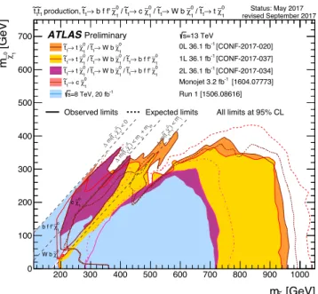
Figure 8: Summary of the exclusion regions for ˜ t

pair production based on 3.2 to 36 fb

of pp collision data taken at √ s = 13 TeV. The dashed and solid lines show the expected and the observed exclusion limits at 95% CL, respectively, including all uncertainties except the theoretical signal cross section uncertainty (PDF and scale) [21].

Figure 8 shows the combination of the results obtained from the final states with different lepton multiplicities. The exclusion contours of all analyses are drawn assuming a branching ratio of 100%

each. For a massless ˜ χ

, top squarks with m

< 950 GeV are exluded at 95% CL. However, all results shown assume that R-parity is conserved, only one-step-decays occur and the LSP is bino-like.

2.1.4 pMSSM-inspired models

It is also possible to interpret results in the phenomenological Minimal Supersymmetric SM (pMSSM) [22, 23]. In case there is a wino-like next-to-lightest supersymmetric particle (NLSP) in addition, for example a ˜ χ

or a ˜ χ

, they are usually motivated to have masses twice as much as the ˜ χ

by models with gauge unification at the GUT scale (cf. Figure 1b). The ˜ χ

can either decay into a Higgs or a Z boson and a ˜ χ

[14]. Figure 9a shows the derived exclusion limit interpreting the results from the 1-lepton final state in the pMSSM. The same selections can also be interpreted for ˜ b

pair production which is sketched as the dashed and dotted grey lines. In case the LSP is a mixed state of bino and Higgsino which is often referred to as the well-tempered neutralino (cf. Figure 1d), the typical mass splitting between the bino and higgsino states is around 20 - 50 GeV. Figure 9b shows the exclusion contours derived from the 1-lepton final state for a rather left-handed ˜ t

.

There are more two-step top squark decays targeted by the ATLAS experiment, e.g. the decay

t ˜

→ t + χ ˜

where the ˜ χ

then further decays into a ˜ χ

and a Higgs or a Z boson. Here, m

< 900 GeV

can be excluded almost independently of m

[24]. The same analysis can also be interpreted in

the scenario where the heavier ˜ t

is produced and then decays into ˜ t

and a Higgs or a Z boson. A

m

< 800 GeV is excluded for the decay via a Z boson, while a m

< 900 GeV is excluded for the

decay via a Higgs boson assuming a light ˜ χ

[24].

8

[GeV]

t~1

550 600 650 700 750 800 850 900 950m [GeV]0 1χ∼m

100 200 300 400 500 600

± χ∼1

b + m

< m mt~

1) M = 2× M2 (

0 χ∼1

m 2×

≈

0 χ∼2

m

≈

± χ∼1

m production, b~1

b~1

, t~1

t~1

Wino NLSP model:

t~1→bχ∼^±₁, t χ∼⁰_1,2 b~1→tχ∼^±₁, b χ∼⁰_1,2 0 χ∼1 W

±→ χ∼1

<0:

µ χ∼⁰₂→ Z χ∼⁰₁, h χ∼⁰₁

>0:

µ χ∼⁰₂→ h χ∼⁰₁ (dominant), Z χ∼⁰₁

= 600 GeV1b ~m = 700 GeV1b ~m = 800 GeV1b ~m = 900 GeV1b ~m

Observed limit exp) 1σ Expected limit (±

<0

µ µ>0

ATLAS Preliminary_-1 = 13 TeV, 36.1 fb Limit at 95% CLs

(a) Wino NLSP model under the hypothesis of a left- handed top squark, where various decay modes are considered with different branching ratios for each signal point. Contours for the µ > 0 and µ < 0 hypotheses are shown as blue and red lines, respec- tively. The grey vertical dash-dotted lines show the corresponding bottom squark mass.

[GeV]

t~1

500 600 700 800 m900

[GeV]0 1χ∼m

200 300 400 500 600

) = 20-50 GeV 0 χ∼1 0, χ∼2 m(

production,∆ b~1

b~1

+ t~1

t~1

Bino/Higgsino mix model:

t~1→bχ∼^±₁, t χ∼⁰_1,2,3 b~1→tχ∼^±₁, b χ∼⁰_1,2,3 0 χ∼1,2 W*

±→ χ∼1

0 χ∼1,2 , Z*/h*

± χ∼1 W*

0→ χ∼3

0 χ∼1 Z*/h*

0→ χ∼2

Observed limit exp) 1σ Expected limit (±

t~L 1≈

t~ t~₁≈t~_R ATLAS Preliminary_-1

= 13 TeV, 36.1 fb Limit at 95% CLs

(b) Well-tempered neutralino model contours for a left- and right top squark are shown separately as red and blue lines, respectively. For left-handed top squark, both ˜ t

/ b ˜

pair productions are considered while for the right-handed top squark, only ˜ t

pair pro- duction is considered.

Figure 9: Expected (dashed) and observed (solid) 95% excluded regions in the plane of m

versus m

for the direct ˜ t

/ b ˜

pair production [14].

2.2 R-parity violating scenarios

In searches for direct ˜ t

production, only the R-parity violating λ

or λ

terms of the superpotential are considered.

For a non-zero λ

, the lepton number is violated, thus the ˜ t

, which is now the LSP, can decay into a bottom quark and a lepton. Searching for this decay, two oppositely charged leptons and two jets where at least one of them is arising from a b-quark are required [25]. For pairing the leptons () and jets (b) correctly, the mass asymmetry m

= | m

− m | /(m

+ m ) (where m

is the mass of b and m is the mass of ) is calculated for all possible permutations and the one with the smallest m

is used. Figure 10a shows that the m

allows for a good background suppression. No excess above SM expectation was found and exclusion limits dependent on the branching ratio of the ˜ t

into b-quark and lepton flavour were set (cf Figure 10b). Depending on the branching ratio, m

< 1.5 TeV can be excluded at 95% CL.

In case of a non-zero λ

, the baryon number can be violated and the ˜ t

decays into 2 jets which

results in a 4-jet final state. The dominant background in this analysis comes from large multi-jet

background arising from various other processes of strong interaction described by the QCD. It is

estimated by a data-driven (DD) ABCD-method as defined in [26] using the mass asymmetry and

the angle between the dijet system and the beamline. With this data-driven estimation, the multi-jet

background is in good agreement with the experimental data as shown in Figure 11a. In case of

a λ

coupling, the ˜ t

decays into bs-quark-pairs and thus, one can require 2 b-tagged jets which

significantly improves the multi-jet rejection (cf. Figure 11b). For the inclusive λ

scenarios, a

m

< 410 GeV is excluded while for the λ

scenarios, a m

< 610 GeV is excluded at 95% CL.